Adopting the parallel strategy in a R&D project task

A D O P T IN G T H E P A R A L L E L S T P A T E G Y IN A R & D

P R O J E Ç T T A S K

A T H E S IS

S U B M IT T E D T O T H E D E P A R T M E N T O F IN D U S T R IA L

E N G IN E E R IN G

A N D T H E I N S T I T U T E O F E N G IN E E R IN G A N D S C IE N C E S

O F B IL K E N T U N IV E R S IT Y

IN P A R T IA L F U L F IL L M E N T O F T H E R E Q U IR E M E N T S

FO R T H E D E G R E E O F

M A S T E R O F S C IE N C E

M oh am ed M ehdi JelassI

S e p te m b e r, 1997

A TH ESIS S U B M IT T E D T O T H E D E P A R T M E N T OF IN D U S T R IA L E N G IN E E R IN G A N D T H E IN S T IT U T E O F E N G IN E E R IN G A N D SC IE N C E S O F B IL K E N T U N IV E R S IT Y IN P A R T IA L F U L F IL L M E N T OF T H E R E Q U IR E M E N T S F O R T H E D E G R E E OF M A S T E R O F S C IE N C E

Mol^

e j Mciv:!.' J eJ

By

M oham ed Mehdi Jelassi

I s о, 55

ѵ)(ц5

I certify that I have read this thesis and that in my opinion it is fully adequate, in scope and in quality, as a thesis for the degree of Master of Science.

Assoc. I^OL· ÎIlkü Ğîirlşr(Principal Advisor)

I certify that I have read this thesis and that in my opinion it is fully adequate.

I certify that I have read this thesis and that in my opinion it is fully adequate, in scope and in quality, as a thesis for the degree of Master of Science.

alim Doğrusöa^^^^

Approved for the Institute of Engineering and Sciences:

Prof. Mehmet Bar ay

ABSTRACT

A D O P T IN G T H E P A R A L L E L S T R A T E G Y IN A R & D P R O J E C T T A S K

M oham ed Mehdi Jelassi M .S. in Industrial Engineering Supervisor: Assoc. Prof. Ülkü Gürler

September, 1997

Funding more than one research team in a R&D project task can increase the chance that at least one of them will achieve a timely breakthrough. However resource limitations imply that the budget allocated to each team declines with the amount of parallelism, reducing the chance that the team will be successful. This tradeoff between level of support and degree of parallelism was explicitly modeled for distinct goals in an environment of uncertain achievements, in order to decide on the number of parallel research teams to fund. In this study which is mainly based on the work done by Gerchak et al, we present the suggested model together with its underlying assumptions and give a detailed mathematical ananlysis. Furthermore, we analytically and numerically analyse the problem of allocating a fixed budget over two research activities and deciding on the number of parallel teams within each activity. Moreover we come out with an analytical result for the general problem of having M activities.

Key words: Research and Development; R&D Project Selection; Parallel Strategy.

P A R A L E L s t r a t e j i y i A R A Ş TiR M A V E G E L İŞ T İR M E p r o j e s i n d e k i b i r g ö r e v e u y a r l a m a

M oham ed Mehdi Jelassi

Endüstri Mühendisliği Bölümü Yüksek Lisans Tez Yöneticisi: Doç. Ülkü Gürler

Eylül, 1997

Araştırma ve Geliştirme projesindeki bir görevde birden fazla araştırma takımına fon sağlamak, bunlardan en azından birini daha kısa zamanda başarıya ulaşması şansını arttırabilir. Fakat, kaynak kısıtlılığı, her takıma düşen bütçenin paralellik miktarıyla beraber azaldığını, ve takımın başarıya ulaşma şansını azaldığını ima eder. Fon sağlanacak paralel araştırma takımlarının sayısının saptanması için, destek miktarı ile paralellik derecesi arasındaki bu tradeoif belirsiz başarılar ortamında ayrık hedefler için açıkça modellenmişti. Temelde Gerchak et a/.’m çalışmasına dayanan bu tez çalışmasında, altında yatan varsayımlarıyla birlikte önerilen modeli sunuyoruz ve matematiksel analizini yapıyoruz. Dahası, sabit bir bütçeyi iki araştırma faaliyetine bölüştürme ve her faaliyette yer alacak paralel takımların sayısını saptama probleminin tahlili ve sayısal analizini yapıyoruz. M aktiviteli genel problemin bir tahlili ile çözümünü de buluyoruz.

Anahtar sözcükler: Araştırma ve Geliştirme, A&G Proje Seçimi, Paralel Strateji.

Special thanks to Neşe Akkaya for suggesting this interesting research topic. I am also greatful to Ülkü Gürler, Mustafa Çelebi Pınar, and Halim Doğrusöz who have been supervizing me with patience and everlasting interest and being helpful in any way during my graduate studies.

Contents

1 Introduction 1

1.1 In trodu ction... 1

2 Literature Review 4

2.1 Literature R e v ie w ... 4

3 The Basic M odel 10

3.1 The Basic M o d e l ... 10

4 Applications Using the Basic Model 17

4.1 Fixed E nvironm ent... 17 4.1.1 Maximizing the Probability that the Best Unit Exceeds

a Fixed Threshold 18

4.1.2 Maximizing the Expected Achievement of the Best Unit 19 4.1.3 Maximizing the Expected Number of Units Exceeding a

Fixed Threshold... 24 4.2 Uncertain Environment... 27

4.2.1 Maximizing the Probability that the Best Unit Exceeds an Uncertain Threshold 28 4.2.2 Maximizing the Expected Number of Units Exceeding a

Random T h r e s h o ld ... 30

5 Extension 32

5.1 Parallel Funding of Research Teams for Two Activities with Equal Threshold Values 32 5.1.1 Interpretation of the Analytical R esu lts... 48 5.2 Generalization of the Analytical R e s u lt ... 50 5.3 Experimental Analysis of a Simple Case 55 5.3.1 Equal Activity-specific Threshold V a lu e s ... 56 5.3.2 Unequal Threshold v a l u e s ... 57

6 Conclusion 59

6.1 C onclusion... 59

A Fixed Environment 63

B Uncertain Environment 65

List of Figures

A .l Optimal Number of Units: Maximizing the Probability that the Best Unit Exceeds a Fixed T h re sh o ld ... 63 A .2 Optimal Number of Units: Maximizing the Expected Achieve­

ment of the Best Unit 64 A . 3 Optimal Number of Units: Maximizing the Expected Number

of Units Exceeding a Fixed Threshold... 64

B . l Optimal Number of Units: Maximizing the Probability that the Best Unit Exceeds a Random Threshold Uniformly Distributed

over [c, d] 65

B.2 Optimal Number of Units: Maximizing the Probability that the Best Unit Exceeds a Random Threshold Distributed by the Truncated Exponential with Parameters a, and ¡ x ... 66 B.3 Optimal Number of Units: Maximizing the Probability that

the Best Unit Exceeds a Random Threshold Distributed by the Truncated Exponential with Parameters a, and ¡j l ... 66

B.4 Optimal Number of Units: Maximizing the Expected Number of Unit Exceeding a Random Threshold Uniformly Distributed over [c, d] ... 67

LIST OF TABLES XI

B.5 Optimal Number of Units: Maximizing the Expected Number of Unit Exceeding a Random Threshold Distributed by the Truncated Exponential with Parameters a, and / u... 67 B. 6 Optimal Number of Units: Maximizing the Expected Number

of Unit Exceeding a Random Threshold Distributed by the Truncated Exponential with Parameters a, and ¡ j ,... 68 C . l Optimal Decision Variables: Equal Activity-specific Threshold

values, very low threshold v a l u e ... 70 C.2 Optimal Decision Variables: Equal Activity-specific Threshold

values, low threshold values 71 C.3 Optimal Decision Variables: Equal Activity-specific Threshold

values, moderately high threshold v a l u e s ... 72 C.4 Optimal Decision Variables: Equal Activity-specific Threshold

values, high threshold v a lu e s... 73 C.5 Optimal Decision Variables: Equal Activity-specific Threshold

values, very high threshold v a lu e s ... 74 C.6 Optimal Decision Variables: Very Low and Unequal

Activity-specific Threshold v a lu e s ... 75 C.7 Optimal Decision Variables: Low and Unequal Activity-specific

Threshold values ... 76 C.8 Optimal Decision Variables: Very High and Unequal

Introduction

1.1

Introduction

A frequent situation faced by the R&D project manager is to identify and explore several alternatives to a particular objective in order to facilitate the selection of the most promising alternative. However, the outcome of any alternative is uncertain, thus making the selection process a difficult one.

Abernathy and Rosenbloom [1] suggested the use of parallel strategies as a tool to deal with this uncertainty in a successful way. They define a parallel strategy as “the simultaneous pursuit of two or more distinct approaches to a single task, when successful completion of any one would satisfy the task requirements.”

Such a strategy can provide better information for a decision, help avoiding the risk of complete failure and induce the building of a broader technological competence for the organization.

More precisely, in R&D projects that are mainly based on human potentials, the R&D project manager usually faces the problem of how to allocate the available budget among research units in order to achieve a specific goal. However, once the parallel strategy is adopted for this case, the R&D project

CHAPTER 1. INTRODUCTION

manager is faced with the question of how many parallel teams to fund. In fact assigning more than one research team to work on the same R&D project must sometimes increase the chance that at least one of them will achieve a timely breakthrough. For example, DEC successfully applied the parallel strategy during the 1980’s. As a result, the company produced a flood of products that increased its revenue tremendously^. Besides, Intel replaced a single design team with four teams working in parallel in the early 1990’s, in hopes of reducing the development time for new generations of computer chips^. Other research-oriented organizations, such as NEC, are also known to use the parallel approaches in the early stages of R&D projects [9]

The decision to fund more than one team is constrained by the potential tradeoff between increased pi'obability of success and increased cost. The probability that at least one of the teams will be successful increases with the number of funded teams in parallel. However, resource limitations imply that the budget allocated to each team declines with the amount of parallelism, reducing the chance that a given team will be successful.

This study will be based on the recent work of Gerchak and Kilgour [6]. Before presenting the structure of the problem to be analyzed, we will review the existing literature in chapter 2.

In chapter 3 we present the basic model suggested in [6] together with its underlying assumptions while revising it for the correctness of mathematical analysis.

In chapter 4, we present the formulations of some problems arising from distinct goals that a decision maker might plausibly want to achieve in a fixed environment as well as in a probabilistic environment. We have analytically and numerically investigated the models provided by Gerchak and Kilgour [6]. Moreover, we have extended the work concerning the probabilistic environment and tried to examine the effect of the uncertainty on the decision taken.

^Business Week, May 4, 1992, p.30 ^The Economist, July 3, 1993, p.22

In chapter 5, we consider another extension of the basic model. There we analytically and numerically, analyze a specific problem of allocating a fixed budget over two activities and choosing the number of parallel teams within each activity. Besides we tried to come out with an analytical result for the same problem, but for M activities.

Finally, in chapter 6, we summarize our findings and make suggestions for further research.

Chapter 2

Literature Review

2.1

Literature Review

Project managers, group leaders, and their associates usually face the problem of choosing among alternative approaches to solutions of technical problems in spite of the associated substantial uncertainty. The most common practice in such situations is the sequential strategy which is the commitment to the best evident approach, and adopting other possibilities only if the first proves unsuccessful. The alternative to the sequential strategy is the parallel one, which is as defined by Abernathy and Rosenbloom [1] “the simultaneous pursuit of two or more distinct approaches to a single task, when successful completion of any one would satisfy the task requirements.” This strategy is one mean by which experienced managers cope with the uncertain nature of the R&D environment. In most situations the advantages of the parallel strategy over the sequential one may not seem to be clear, while its additional costs are quite evident. However by adopting more than one approach to a single task, the manager

• avoids the risk associated with determining a-priori which of the several uncertain approaches that will perform best.

• can obtain sufficient information that allow him to come out with a better choice among approaches,

• can protect himself against the risk of complete failure, and

• can help building a broader technological competence for the organization by stimulating competitive effort.

The basic study in the available literature that focuses on the benefits that can be gained from the adoption of the parallel strategy approach is the one conducted by Abernathy and Rosenbloom [1]. In order to benefit from these advantages, in [1] they tried to facilitate the explicit evaluation of the sequential and the parallel strategies by decision makers in real life projects and thus decide when the parallel strategy approach is justified over the sequential one. That is the decision maker is faced with a complex development project that must be undertaken in steps or stages. At each stage the decision maker must decide on following the sequential or the parallel strategy for the completion of the task. Besides they generalized more usefully about the structure of this decision problem by distinguishing between two broad categories for the use of parallel strategies: The parallel synthesis strategy and the parallel engineering strategy. The first category is most often found in the early phase of a project. Thus the parallel synthesis strategy is typically a means of gaining information and maintaining options so that the best path may be selected for subsequent development. Thus in this category

• the uncertainty is broad,

• the cost of information is relatively low, and

• there may be only a limited commitment to further work.

Whereas the second category occurs in a larger stage of the development process, when great deal of information has already been acquired and there is little chance that the total program will be abandoned. Thus in this category

• the bounds of uncertainty are more definite, • the information cost is relatively high, and

• there is a strong commitment to satisfy development objectives.

With the parallel engineering strategy, in contrast to the synthesis strategy, the decision maker usually is committed to bring the development project to a successful completion. If he chooses only the preferred approach and it does not prove acceptable, then he must look for a new solution. This implies time delays and higher costs. Whereas by following a single unsuccessful approach in the synthesis strategy, the consequences are somewhat different. An incorrect choice may mean that the program is abandoned, since the benefits that would be offered by a different approach may never be demonstrated. Abernathy and Rosenbloom [1] focussed their work on the parallel engineering strategy, and came out with the following characteristics that describe the structure in which a parallel engineering strategy may be warranted;

CHAPTER 2. LITERATURE REVIEW

6

1. The task is well defined, typically as a set of performance requirements that the various approaches must attain or exceed. There is explicit uncertainty about the outcome of a given approach as measured on a given performance dimensions.

2. There may be a significant probability that any one of the approaches will not provide an acceptable solution, since the solution is constrained by many requirements.

.3. Satisfactory completion of the task is a primary goal, and the cost of failing to do so is high in respect to the direct cost or differential worth of alternative approaches.

4. Two or more approaches that may satisfy the task can be identified. At least one of the approaches has an uncertain outcome. The uncertain aspects are typically the feasibility, the completion time, and the specific characteristics of technical performance.

5. One of the potential approaches may usually be identified as preferred. The required decision, then, is whether to add one or more approaches in parallel to this first one.

The general model suggested by Abernathy and Rosenbloom [1], deals with the case where there are two possible approaches to a single remaining stage of development for a well defined task. Two strategies are to be compared: The parallel strategy where the two approaches are initiated at the same time, and the sequential strategy where the second approach is initiated only if the first approach fails. Their suggested criterion for the choice between the two strategies is to maximize the expected value of the difference between the value of the task outcome which is dependent upon performance, and completion time, and the cost of development to produce that outcome, which is determined by many choices, some of which influence the task performance as well as its completion time. They defined three functions in order to relate a given approach outcome to the criterion measure:

1. A loss function, representing opportunity costs of delays in project completion through obsolescence, diminished competitive advantage, and so forth.

2. A second loss function, representing out-of-pocket costs incurred by extension of project duration. These overhead expenditures, penalties, and the like.

3. A function which evaluates the worth of the performance outcomes of each approach.

The first two functions must be estimated in analysis of a real situation, whereas the likelihood of various project outcomes are suggested to be estimated using the judgemental probability distributions.

Once these value functions are made explicit, the expected benefits of the parallel strategy over the sequential one are evaluated.

CHAPTER 2. LITERATURE REVIEW

First, when both approaches succeed, the parallel strategy offers the option of picking the one that turned out to be better. Although the first approach was initially preferred, the second may be completed earlier or may actually perform better.

The other benefit of a parallel strategy is that it offers a means of avoiding late project completion when the preferred approach fails and the second succeeds

The expected value of these two benefits are compared to the differential expected direct cost to decide whether the parallel strategy is justified over the sequential one or not. The parallel strategy is justified if its differential economic benefits are greater than its differential cost. However, the decision to choose among the parallel and the sequential strategies is highly dependent on the availability of I’elevant information, on the accuracy of estimating input data, and on selecting the factors governing the choice of a strategy. The basic model suggested by Abernathy and Rosenbloom [1], avoids all the disadvantages previously mentioned and considers only precise input data, which are the total available budget and the threshold value to be achieved by the R&D activity.

Most of the available literature deals with the problem of selecting among alternative project tasks. Here, the R&D project is considered to consist of several stages, where each stage may be completed by undertaking one or more tasks. In [4] Bard has pointed out the troublesome aspect of this problem. In fact among the project task, both systematic and statistical dependencies exist which do not conveniently permit a standard mathematical programming formulation [3], [13], [15]. These may take the form of overlap in resource utilization, technical interrelationships among task outcomes, or externalities where the value contributions or joint performances of several tasks may be nonadditive [10]. Consequently, the problem has been modeled as a probabilistic network [11], [14] and solved with a heuristic embodying simulation within a dynamic program. Numerous quantitative models for selecting research and development projects have been developed and reported

in [3]. An evolutionary process has taken place resulting in a number of mathematically sophisticated approaches for R&D project selection with varying degrees of proven effectiveness.However in our study, the R&D projects considered are those which are mainly consisting of only one task that is mostly dependent on human potentials.

Taylor et al [16], along with Keefer [10], have recognized that project performance is rarely a linear function of resource utilization. Realistically, success probabilities and expected monetary returns typically increase, but at a decreasing rate with the level of effort. Added complexity aside, the incorporation of such nonlinearities in the model may go a long way in building management’s confidence in the analytic results [12], [15]. Along with this fact, Gerchak and Kilgour [6] suggested that the achievement is exponentially increasing with the level of resource support, as it will be seen in chapter 3.

Chapter 3

The Basic Model

3.1

The Basic Model

The question of how many uniform teams to fund in parallel constitutes the concern of the study conducted by Gerchak and Kilgour [6]. In their work the research teams are assumed to be uniform with respect to their potential achievements as measured by the achievement level probability distributions. Specifically, it is assumed that the achievement level probability distributions of the teams are identical given their funding is done on an equal basis. Moreover, it is assumed that the performances of funded teams are independent of each other. These assumptions will be further elaborated.

In order to determine the number of research teams to be funded in parallel, the tradeoff between level of support and degree of parallelism is modeled for distinct goals that a decision maker wants to achieve in different operating environments.

Firstly, the case of a decision maker operating in a fixed environment is considered. In such an environment the aimed level of achievement is explicitly specified in advance, and the performance levels of rivals are known. Gerchak and Kilgour [6] addressed three goals that a decision maker might certainly

want to achieve in this fixed environment. These are:

1. Maximize the probability that the best unit exceeds a predetermined threshold.

2. Maximize the expected achievement of the best unit.

3. Maximize the expected number of units exceeding a fixed threshold.

Next, the case of a decision maker operating in an uncertain environment is considered. In this situation, the decision maker knows the amount of resources its competitors have allocated to the activity, and how they were allocated, but is uncertain how successful the competitors will be. Here, the distribution of the threshold is derived using the knowledge on the investments by the competitors. In a sense, this distribution stands for the achievement level of the competitors. Two goals that a decision maker might certainly want to achieve in this uncertain environment can be stated as follows:

1. Maximize the probability that the best unit exceeds a random threshold. 2. Maximize the expected number of units exceeding a random threshold.

The first goal was studied by Gerchak and Kilgour [6], whereas the second one is studied in this work.

Finally, the problem of allocating a fixed budget over two activities and choosing the number of parallel teams within ecich activity was dealt with. In this case the decision maker’s goal is to maximize the expected number of activities in which the best unit exceeds an activity-specific threshold.

In achieving each of these objectives, the decision maker is assumed to have a fixed budget B, which will be equally divided among the funded teams.

The random future achievement of the research team i, will be denoted by Xi. Numerous studies modeled the achievement in a R&D project task by

CHAPTER 3. THE BASIC MODEL

12

assigning judgemental discrete values for the probability of success [1], [16], or just view the achievement as success or failure [15]. In fact, some research oriented organizations such as the National Science Foundations can measure the research output by some continuous scale. It can be the case that one or several research teams are funded by such organizations in order to strive for a high or a low value of achievement. Research teams may be working hard to perform a high value of achievement. For instance, improving certain product characteristics such as, memory capacity of a chip, reliability of an electronic component, etc .Thus their performance is measured in terms of these quantitative characteristics, where high values of achievement are looked for. Or, research teams may be working hard to perform a low value of achievement. For example, noise in a certain electronic signal, the time taken by a certain drug to act on the body, etc . Thus their performance is measured in terms of these quantitative characteristics, where low values of achievement are desired. In this study, we shall focus on the high value scenario.

In what follows as mentioned previously the achievements of the research teams are assumed to be mutually independent. The decision maker may impose the independence between the research teams funded in order to avoid the negative effects associated with the fact of competing for the same goal. The independence condition in this situation may enable the teams to use fully their own potential and thus increase their efficiency. In addition to that the negative effects on the motivation and the willingness of the research teams, such as losing hope are certainly avoided. However, we must admit that this independence assumption is not realistic in some situations. Athletes who train together, for instance, may motivate each other to do better performance. Thus, their resulting achievement levels would be positively correlated, and might further be positively related to the number of parallel units funded, mitigating the negative effects arising form the decrease in the unit’s funding level. The analysis using the independence assumption is an important first step and can be considered as the base case. Not only would it make the analysis of the mathematical analysis easier to carry out, but it would also provide a lower bound on the optimal number of parallel units to fund when

positive correlations are available.

Moreover, the achievements of the research teams are assumed to have identical probabilistic distributions. This assumption is realistic in many R&D programs, such as those in the pharmaceutical industry. In this case a company is likely to divide personnel and resources into teams of equal capabilities and assign them to the same goal to compete for. In addition to that, once it is decided on adopting the parallel strategy for a certain R&D activity, the decision maker won’t fund research teams whose potentials differ considerably. In fact the decision maker assumes that research teams have equal potential to achieve a certain goal, and then decide on the number of parallel teams to be fund. However, we must admit that judging about the potential of a research team is not a straightforward process.

If we measure the performance of the team by the achievement of a given threshold, then we will observe that the team will achieve a lower threshold with considerably higher probability than a higher threshold. Therefore, the exponential family is a good candidate to describe the probabilistic achievement of a given team.

Because of the total research budget constraint, the chance that a given team will achieve a fixed threshold T decreases with decreasing budget allocation to the team. Therefore, the team’s achievement probability density function is thought to be a function of a, the fraction of budget that the research team receives. Here, we assume that each team receives an equal fraction of the total budget, allowing for an equality in potential achievements of the teams. Thus, we have a = Bjn, where B is the total budget to be allocated equally to the research teams, and n is the number of research teams to be funded. Without loss of generality, we can set H = 1.

In order to reflect this observation in the achievement distribution, the rate of the corresponding exponential distribution. A, should be defined as a function of a. Thus the density function of the achievement distribution becomes:

CHAPTER 3. THE BASIC MODEL

14

with the cumulative distribution function:

F{x; a) = I — e for a; > 0

0 for a; < 0

(

2

)

Thus, letting Yn be the achievement of the best unit, we have = max{Xi, ...,Xn)·

Since X i,..., Xn are i.i.d,

P (Y ^ < V ) = [F (y ,a )f .

It is important to note that the achievement distribution F{x] a) should be a decreasing function of a for any fixed x, since, as mentioned above the probability that a team will be successful decreases as the fraction of budget received by each team decreases, ( or equivalently the number of funded teams increases ).Thus, A(a) should be a decreasing function of a. Furthermore, the fact that the expected performance of any given research team, 1/A(a), should increase with increasing budget allocation per team indicates that A(a) should be decreasing in a. This fact is reflected in the following form of A(a) suggested in [6]:

A(a) = La ", ₍₃₎ where a is a sensitivity parameter, with 0 < a < 1, and L > 0. The closer a

to 1 the more sensitive the research team achievement to budget allocation. Although we are not restricted in the choice of A(a) to the above form, it is important to note that Gerchak and Kilgour did not report anything in [6] about the functional form of A(a). However we believe that this functional form of A(a) must be explicitly stated.

Firstly, A(a) should be strictly decreasing in a, like in the above choice, for the following reasons. For any two real numbers ai, and Oa, such that Oi < a2,

F{x',ai) — F { x ; a2) must be nonnegative for a given a; > 0. It follows that A(ai) > A(a2), implying that A(a) is decreasing in a.

In order to verify that A(a) has to be necessarily strictly decreasing in a,

we have analyzed the case where A(a) = a — 1/n. Maximizing the probability that the best unit attains a fixed threshold T translates into

max 1 [F (T ; a)]" = max 1 (1

-= max 1 — (1 —

— max 1 — (1 — e

uEZ\

Letting B — t we have

which is equivalent to,

max 1 (1

-nEZ\

min (1

-nEZ^

Treating n as continuous and taking the derivative of this objective function with respect to n results in the following expression:

or equivalently,

(1 — a:)"“ ^ {(l — o:)log(l — x) + a; log a:}, where x =

This expression never vanishes to zero. It is strictly smaller than zero for all values of x.

Therefore A(a) should be strictly decreasing in a, to assure the existence of a solution to ¿ ( 1 = 0.

Moreover, by the requirement that

CHAPTER 3. THE BASIC MODEL

16

implying that

A(a) > 0.

Furthermore, the choice of A(a) should satisfy the following conditions:

1. lima_o A(a) > 0,

2. A(a) is continuous in a.

The first property is necessary to reflect the dependence of the achievement distribution on the magnitude of funding, whereas the second property will be necessary in optimization process as will become obvious in the following chapter.

Applications Using the Basic

Model

4.1

Fixed Environment

In this section, the environment in which the decision maker is operating is assumed to be fixed. That is, the criteria for assessing achievement are a-priori and explicitly specified. The outside environment which consists mainly of competitors does not have any effect on these criteria. Thus based on the model presented in the previous chapter, three problems arising from distinct goals that a decision maker might plausibly Wcint to achieve in a fixed environment are addressed by Gerchak and Kilgour [6]. These are

1. Maximize the probability that the best unit exceeds a predetermined threshold.

2. Maximize the expected achievement of the best unit.

3. Maximize the expected number of units exceeding a fixed threshold.

We have revised these problems for the correctness of mathematical analysis, and provided further analytical and numerical results.

CHAPTER 4. APPLICATIONS USING THE BASIC MODEL

18

4.1.1

Maximizing the Probability that the Best Unit

Exceeds a Fixed Threshold

In this section we will summarize the results of Gerchak and Kilgour [6] on n*, the optimum number of research teams in parallel that maximizes the probability that the best unit exceeds a fixed threshold, and tried to come out with some analytical results, as well as some numerical results.

The probability that the best unit attains a predetermined threshold T is given by

P{Yn > T ) = 1 - [F{T·, 1/n)]” . The problem is

which is equivalent to.

max P{Yn > T),

n e

min 1/n)]” ,

n £

For the suggested achievement distribution we have, P (F„ > T ) = 1 [1

-=

1

[1

-Thus the problem is to find out the number of teams in parallel, n* that maximizes the above expression. That is

n* = arg min [1 —

n e

For the case of the activity being highly sensitive to resource allocation we have come out with the following result.

Proposition 1 For a = 1, if LT > In 2, then n = 1 maximizes the probability

that the best unit attains a fixed threshold T .

Proof:

For a = 1, the expression that we want to minimize over n is. /( n ) = (1

-Let LT = x, then the above expression transforms into

i(n) = (1 - e - ” )".

Treating n as continuous, the derivative of f{n) with respect to n is

(1

-nxe

1 — e" + l n ( l - e - " " ) l ·

This derivative is non positive for nx < In 2, and it is nonnegative for nx > In 2. Since /( 1 ) > 0, then /( n ) is an increasing function of n when nx > In 2. Now the smelliest value that n can take is 1. Therefore for LT > ln2, n = 1 minimizes /( n ) , thus maximizes the probability that the best unit exceeds a fixed threshold T. |

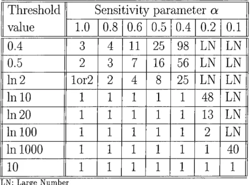
Note that when the research team’s achievement is very sensitive to budget allocation, and LT = ln(a) where a > 2, the optimal decision is to fund only one team, whose probability of achieving the threshold value of T is 1/a. Thus, the probability of exceeding an activity-specific threshold value, decreases as that threshold value increases. The numerical calculation of n* presented in Table A .l, reveals that n* is decreasing in a. Moreover, it is decreasing in

T. When the sensitivity parameter is very low, that is when a —»· 0, and the threshold is not very high ( T is at most equal to In 1000), the number of parallel teams that maximizes the probability that the best unit exceeds a fixed threshold increase tremendously. This is due to the fact that resource allocation does not affect the research team’s performance. So increasing the number of parallel teams must increase the chance of reaching that performance.

4.1.2

Maximizing the Expected Achievement of the

Best Unit

In this section we will summarize the results of Gerchak and Kilgour [6] on n*,

the optimum number of research teams in parallel that maximizes the expected achievement of the best unit is to be determined. Besides we performed further

CHAPTER 4. APPLICATIONS USING THE BASIC MODEL

20

analytical work on the suggested problem, that supports the numerical analysis performed.

Thus, our aim is

Where,

max E[Yn] nez^

Yn = max X;.

K i < n

Since Xi are nonnegative random variables, we have

POO E[Yn] = / P { Y n > y ) d y Jo POO = / [i - P ( y . < y)] dy Jo POO = / 1 - [F(?/; 1/n )]" dy, Jo setting jB = 1.

For our exponential family F { y , l f n ) = 1 — it is well known ( e.g Arnold et al. [2] ) that

E[Yn] =

Therefore, the problem reduces to

1 " 1 1 Ln^ k' 1 " 1 - y - · , 0 ^ 1. (1) max , / , . nez+ Ln°‘ k

It is important to note that for a = 1, E\Yn] is decreasing in n, i.e. in the case of high sensitivity to budget allocation, the expected achievement of the best team increases as the number of funded teams decreases ( or equivalently as the fraction of budget assigned to each team increases ). In the following part we wanted to check whether E[Yn] is decreasing in n for all values of a

or not. In fact this was not observed for all values of a. By simulation, it is found that E[Yn] {for T = 1) is strictly decreasing in n, only for the values of

a satisfying a > 0.5848. Thus, we tried to check this fact analytically in the following parts.

A lower Bound on the Value of a by Working out a Lower Bound for E[ Yn]

Since E\Yn] is not decreasing in n for all values of a in (0,1], it is important to verify the simulated lower bound value of a also in a mathematical setup. This is accomplished in the following by working out a lower bound for E\Yn\

and then providing a lower bound on a such that E\Yn] is strictly decreasing in n. We start by analyzing the sum in [8].

We have

where

t \ = C + lnn + i - E

fc=l

2n

^ - 1)

1 H

A k = Y a;(l — x ) { 2 — a;)(3 — x ) . . . i k — 1 — a;)

k Jo d x a n d C - - + V — Thus, for T = 1, _ ___' ^ 4 ( + k — 1) — k\ n" I 2 2n 2n ^ ^ y k\n{ n + l)...(n + A; — 1) Considering the numerator of the fraction within the above sum, we have

n { n + l ) . . . { n + k - 1) - k\ = ^ - A:! ( n - i ) ! H I l - H n — I

=

;

+

i - n > 0 .

n — 1

CHAPTER 4. APPLICATIONS USING THE BASIC MODEL

22

Thus, a lower bound for E[ Yn] is

Taking the derivative of the right hand side with respect to n results in;

In order for the lower bound of E[ Yn] to be decreasing in n, we should have: - - ( l + - - T --- o:lnn + l < 0 2 V 77./ 2 n That is, 2t7 - 1 < a. 1 + 77 + 2?7 In 77

The left hand side of this inequality is increasing for n < 1.426, and it is decreasing for n > 1.426.

Therefore, for a G (0.539,1], £^[5^] should be strictly decreasing in n.

A lower bound on the value of a by working out an U p p e r Bound for E [ Y n ]

In this part, E[ Yn] is approximated by an upper bound in order to come out with a lower on a such that E[Yn] is strictly decreasing in n.

By the presentation in the foregoing section we have, 1 N Obviously, Afc = — y o;(l — x ) { 2 — x')(3 — x ) . . . ( k — 1 — .r) d x . (1 — x ) { 2 — .'c)(3 — x ) . . . { k — 1 — x ) < 1 . 2 . . . { k — 1) and, therefore, 1 N y / x i l — x ) { 2 — a;)(3 — x ) . . . ( k — 1 — x ) d x < y

f

and

.

Taking the derivative of the right hand side with respect to n we obtain

„ - “ - 1 ( 1 -p s{k)) - a ln n + 1 + ^ ( - « - 1)^

In order for the expression on the right hand side to be strictly decreasing in n, we should have: (1 + S{k)) - a \ n n + l + ^ i - a - 1) < 0. 2 zn That is, or equivalently

2n - 1

This expression is increasing in n for n < 1.664, and it is decreasing in n for n > 1.664.

CHAPTER 4. APPLICATIONS USING THE BASIC MODEL

24

Note that the lower bound that we suggested for E\Yr^\ in the foregoing provides us with a closer lower bound on the simulated lower bound value of a, than the one derived in this section.

Examining Table A .2, we notice that the experimental results are in line with the previous analytical work. In the sense that E[E„] is strictly decreasing in n for some values of a. In fact, E\Yn] is maximized at n* = 1, is equivalent

to E\Y-n\ is decreasing in n. Thus as it is shown Table A .2, for the values of a

that cire more than 0.5, E\Yn] is strictly decreasing in n.

Besides, the optimal number of parallel teams that maximizes the expected achievement of the best team is decreasing in a. The less sensitive the activity is to budget allocation, the more teams are assigned to that activity. Furthermore, as a ^ 0, that is when the activity is not sensitive at all to resource allocation, the optimal number of parallel teams that maximizes the expected achievement of the best unit increases tremendously. This can be seen from the analytical form of E[E„].

E[Yn] U-.0 = E 1

k = l

The above expression is an increasing function of n. Thus the largest possible

n will maximize it.

4.1.3

Maximizing the Expected Number of Units

Exceeding a Fixed Threshold

In this section we summarize the work done by Gerchak and Kilgour [6]. The expression, M „(T ), for the expected number of teams exceeding a fixed threshold T is derived, in order to find n*, the number of teams that maximizes

Mn{T). In addition to that, we have analytically corrected a statement reported in [6], and provided numerical results as well as some analytical ones. Now, Suppose that n equivalent research teams are employed for the project and that all are funded on an equal basis. Then the probability of any one of those n teams to exceed the threshold T is given by F{T·,

Thus, among a fixed number of teams n, the number of teams exceeding threshold level T is a binomial random variable with parameters n and

F{T] 1/n ), and the expected, number of teams attaining threshold level T is

Mn{T) = nF(T-l/n).

By the choice for F we have

MniT) ne- \ { l / n ) T

with A (l/n ) = Tn". Now the problem of maximizing M „(T ) can be stated as max

n£Z^

Letting ^ we have

max nO^ nez^

Treating n as continuous, and taking the derivative of the objective function with respect to n we get

^ n r “ = r “ (l + a n “ In 0).

an

Equating the right hand side to 0 and solving for n results in the unique critical value no given by

To check whether the extremum is a maximum we analyze the sign of the second derivative

(P

dn"^

n9^ = an°‘

InO {1 F a A OiiClnO).

Since 0 < ^ < 1 , l n ^ < 0 and the sign of the second derivative at Hq is of opposite sign as compared to (1 + a + o-Uq 1ii0), which is positive. Thus,

dn^ n9^ _n=7l0 < 0 ,

and it follows that n^"“ attains its maximum at n = no- Although Gerchak and Kilgour [6] stated that the smaller a the larger uq, it is found out that this

CHAPTER 4. APPLICATIONS USING THE BASIC MODEL

26

does not hold for the entire range of possible values of a. In fact, taking the derivative of the expression for no with respect to a we get

dno da — ( da \a\n6j - 1 y / " ( In ( - ^ ) 1 a ln ^ y a^ a^

Since 0 < ^ < 1, In^ < 0, the first term in the above expression is positive. Now, for no to be decreasing in a, we must hcive ^ < 0, which implies that we have In ( - ^ ) a^ a^ < 0 - I n a\n9 < 1 ln(—a ln ^ ) < 1 —aXxiO < e e ln0 —a > -—- where 6 = e -a > a < - L T e

If

Thus, no is a decreasing function of cc if o; < where e is the base of the natural logarithm. Furthermore, we came out with the condition under which the parallel strategy is not justified over funding only one team in order to maximize the expected number of units exceeding a fixed threshold T. This is given in the foilwing proposition.

Proposition 2 For o; > n — I, maximizes the expected number of units exceeding a fixed threshold T.

Proof:

Treating n as continious, the derivative of n0'^°‘ with respect to n must be nonpositive. Thus,

0” “ (1 + a?r“ ln0) < 0, implies that

> -r;^· - LT

Since the smallest value that n can take is 1, then the above expression translates into,

Q' > 1

LT'

Thus when a > n = 1, maximizes the expected number of units exceeding a fixed threshold T. |

The above result is also seen through Table A.3. Besides, we notice that the optimal number of parallel teams that maximizes the expected number of units exceeding a fixed threshold is decreasing in a, the sensitivity parameter, and T, the threshold value. When the activity threshold value is very high, funding more than one team in parallel is not justified over funding only one team for most of a values.

4.2

Uncertain Environment

In this section, the environment in which the decision maker is operating is uncertain. These situations correspond to scenarios where the decision maker knows the amount of resources its competitors have allocated to the activity, and how they were allocated, but is uncertain how successful the competitors will be. Thus, the criterion for assessing achievement are not a- priori known, but their probability distribution is known. So based on the model presented in the previous chapter, two models arising from distinct goals that a decision maker might plausibly want to achieve in an uncertain environment are addressed in [6]. These are

CHAPTER 4. APPLICATIONS USING THE BASIC MODEL

28

1. Maximize the probability that the best unit exceeds a threshold that is random with known distribution.

2. Maximize the expected number of units exceeding a random threshold.

The first goal was modeled, and numerically explored by Gerchak and Kilgour in [6], for the threshold being uniformly distributed. We have investigated the case when the threshold value is distributed by the truncated exponential. In addition to that we have modeled the second goal for the threshold value being uniformly distributed, as well as being distributed by the truncated exponential. Besides, we tried to investigate the effect of the uncertainity of the outside environment on the decision taken.

4.2.1

Maximizing the Probability that the Best Unit

Exceeds an Uncertain Threshold

The probability that the best unit exceeds a random threshold whose distribution is given by H(t) is P { Y n > T ) = / P { Y ^ > t ) d H { t ) Jo /* + 00 = / { l - l f i f ; ! / « ) ] “ ) J 0 /*+00 . = 1 - / [ F ( f , l l n ) f dH(t) Jo

Maximizing the probability that the best unit exceeds a random threshold is equivalent to

mm / ( f ( i ; 1/n)]" dH(t). Jo

For our exponential family, the problem transforms into

min /

(1

‘‘m

Gerchak and Kilgour [6] have suggested that the threshold value is uniformly distributed. That is the threshold value is equally likely to be any value within

a certain interval [c, ci]. So, the density lunction of the threshold value is: -1 - for c < t < d

/ ( 0 = i ,, . 0 otherwise Thus the problem is

which is equivalent to f d mm ne^+ Jc — Ln °‘ t \ n cl — c-dt, rd mm / (1 -Jc — L n ^ t \ n_{)" dt.}

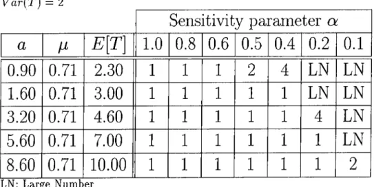
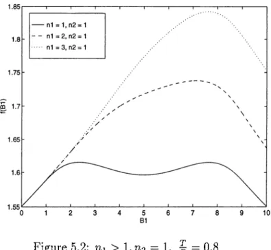
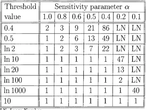
For different threshold Vcilue intervals and sensitivity parameters, some values of n* that maximizes the probability that the best unit exceeds a random threshold are presented in Table B .l. The effect of the outside environment uncertainty on the decision of funding parallel teams can be concluded froiii the comparison of Table A .l and Table B .l. In fact when the activity is sensitive to resource allocation ( a > 0.-5 ), and when the expected threshold value is high ( E[T\ > 2.3), the decision is the same. Whether the outside environment is fixed or probabilistic the decision is to fund only one team for that activity. However, when the activity is not sensitive to resource allocation, the decision is to assign more teams in parallel when the outside environment is pi'obabilistic.

We thought that the truncated exponential distribution is a good candidate to describe the probabilistic threshold values. In fact very low threshold values may not be considered by a decision maker. However, high threshold values are considered with decreasing probabilities. Thus, the threshold value’s density function is given by = t > a . Thus, we have m i n / ( 1 di. which is equivalent to min / (1 - dt. Z -h »/ Cl

CHAPTER 4. APPLICATIONS USING THE BASIC MODEL

30

For different parameters of the threshold distribution, and sensitivity parameters, some values of n* that maximizes the probability that the best unit exceeds a random threshold are presented in Table B.2, and Table B.3. Comparing these two tables, we notice that when the activity threshold value variance is high more teams are assigned to that activity. Thus the higher the variance of the threshold the more teams are allocated to that activity to deal with this outside uncertainty. Besides whether the threshold value is uniformly distributed or truncated exponentially distributed similar remarks are observed when compared to the fixed environment.

4.2.2

Maximizing the Expected Number of Units

Exceeding a Random Threshold

For a fixed n, the number of units exceeding a threshold level T is binomial with parameters n and probability of success given by

r+oo /* + 00

P ( X > T ) =

/

PiYr, > t) dH(t)

=

{l-F(t-,l/n)}dH(t).

Thus, the expected number of units exceeding a rcindom threshold is /*+00

M (n ) = n / {I - F{t-, l/n)} dH{t) Jo

For our exponential family, it is

r+oo M(n) = n / {1 — (1 J 0

) dH{t)

_dH{t)

Thus the problem is

max M{n). nez^

For the threshold being uniformly distributed over [c, d], M{n) is given by

M(n) = n

^ f^-Ln^c _ ^-Ln

L { d — c )

So the problem translates to

max .

nez+ V >

For different threshold value intervals and sensitivity parameters, some values of n* that maximizes the expected number of units exceeding a random threshold are presented in Table B.4. Comparing Table A.3 and Table B.4 we notice that more parallel teams are funded in the case when the environment is probabilistic.

For the threshold value being distributed by the truncated exponential on [a, + c o ), the problem transforms into

^4-00 /*+oo M { n ) = n / dt J a /‘ + 00 = dt J a ,g-Ln“ a Ln^ + ¡.i

For different parameters of the threshold distribution, and sensitivity parameters, some values of n* that maximizes the expected number of units exceeding a random threshold are presented in Table B.5, and Table B.6. Comparing these two tables, similar results to the previous section are obtained.

Chapter 5

Extension

5.1

Parallel Funding of Research Teams for

Two Activities with Equal Threshold

Values

A common situation faced by the decision maker is to allocate a fixed budget over several activities. Then in order to take advantage of the parallel strategy he must decide on the number of parallel teams to be funded in each activity. So, once the amount of budget to be allocated to a specific activity is determined, it is assumed that it is divided equally over the determined number of parallel research teams working on that activity.

Let j = 1 ,...,M be the potential activities. Let B be the total available budget to be allocated over the M activities. Let Bj be the budget allocated to activity j.

Then we have,

M

E

i=l

Let rij be the number of parallel research tecuns working on activity j. So, within each activity j for which Bj > 0, the budget will be divided equally

among the nj teams. The achievement distribution of a single team pursuing activity j is then Fj{x : Bjinj), and thus the achievement distribution of the best unit within activity j is {Fj(x : Bj/nj)}'^T Thus the probability that the best unit exceeds an activity-specific threshold Tj within activity j is

According to Gerchak and Kilgour [6], a plausible goal is to maximize the expected number of activities in which the best unit exceeds an activity-specific threshold Tj. So the generalized formulation of this problem as suggested in [6] is as follows M 3 = 1 subject to M i=l where

j = are the potential activities,

Bj is the budget allocated to activity j, В is the total available budget,

Tij is the number of parallel teams to be funded for activity j,

1 — [Fj{Tj; Bj/nj)]"^^ is the probability that the best team in activity] exceeds an activity-specific threshold Tj.

For our exponential family the objective function can be restated as

M шах 52 " [I ~ l ... njw ^ which is equivalent to M mm _{E H}

In this part we have treated the case when M = 2, and T\ = = T. That is the decision maker must allocate the available budget over the two activities

CHAPTER 5. EXTENSION

34

on the number of parallel teams pursuing each activity in order to maximize the expected number of activities in which the best unit exceeds the activity- specific threshold T. Besides, without loss of generality, we have fixed Li = 1,2 = 1 in order to facilitate the mathematical analysis. Moreover we decided on the condition that ai = « 2 = 1, to reflect the common situation that the

research team achievement is very sensitive to budget allocation. That is, the closer the sensitivity parameter, a to 1, the higher the expected performance of the research team. This problem is reflected into the following

where.

and

min f { B i ) = [1 - + [1

-0 < Bi < B,

T > 0.

Proposition 3 For ^ > ln2, f { B i ) at ni = ri2 = I is smaller than or equal to f{B\) at ni = 1 and U2 > 1 for all values of 0 < Bi < B.

Proof:

f{ B i ) at ni = n2 = 1 is equal to

(1

(1

-Let’s fix ni = 1, and consider any H2 > 1, then the corresponding f{ B i ) is equal to

Subtracting f { B i ) at ni = rz2 = 1 from f{ B i ) at rii = 1, and U2 > 1 results in

_ g-(n2/(s-Si))T^n2 _ Let

= X, B - B i

then the previous expression translates into (1 _ e~n2xp _

where x > 0.

The above expression is equal to 0 when n2 = 1.

Treating U2 as continuous, the derivative of the above expression with respect

to ri2 is

(1

U2xe— 7l2X

+ ln(l - \ . _ ^ — n2X

This derivative vanishes when H2X = In 2. Moreover the difference is decreasing in U2 when U2X < In 2, and it is increasing in U2 when U2X > In 2.

Now since the smallest value that U2 can take is 1, then,

(1 _ ^-n2X^n2 _ is always nonnegative for all values of n2 > 1 if

T

X = > In 2.

B - B x

Thus, for all values of 5 i , where 0 < < 5 , f { B i ) at ni = U2 = 1 is less

than or equal to f { B i ) at ni = 1, and ri2 > 1 if

T

t;— > ln2.

B - B i ­

ll ow, since 0 < jBi < B, then the above condition is reflected in the following

one,

T

^ > l n 2 .

Therefore, for ^ > ln2, f { B i ) at ni = n2 = 1 is smaller than or equal to

f { B i ) at ni = 1 and n2 > 1 for all values of 0 < Bi < B .

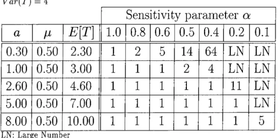
The previous analytical result can be clearly observed through a numerical example. We fix B — 10, and T = 8, thus ^ = 0.8, which is greater than In 2. Then for some values of ni, and U2 satisfying the condition of Proposition 3,

we plot the corresponding f{ B i ), and compare it with the plot of f{ B i ) at m = U2 = 1. These are presented in Figure 5.1. It is clear that for the whole

range of Bi, f { B i ) at nj = U2 = 1 is less than or equal to all other / ( 5 i ) ’s

CHAPTERS. EXTENSION

36

Figure 5.1: ni = l , n2 > 1, ^ = 0.8

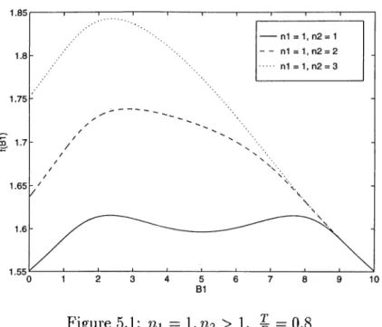
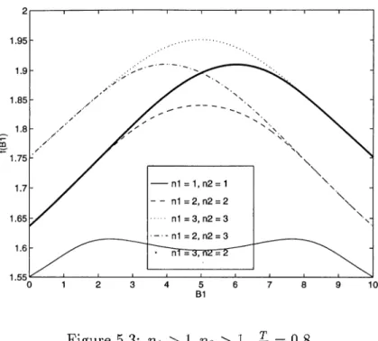
P r o p o s itio n 4 For ^ > ln2, f { B i ) at n\ = ri2 = I is smaller than or equal to f { B i ) at ni > 1 and U2 = 1 for all values of 0 < Bi < B .

P r o o f:

Now let’s fix U2 = 1 and consider any ni > 1, then subtracting f { B i ) cit

rii = U2 = 1 from f { B i ) at ni > 1, and ri2 = I results in

(1 - e-im/Bi)TyH _ (1 _

Let — X, then the above expression translates into

where a; > 0.

The above expression is equal to 0 when 7гı = 1.

Similarly, Treating ni as continuous, the derivative of the above expression with respect to rii is

(1

-This derivative vanishes when riix = In 2. Moreover the difference is decreasing in ni when n-ix < In2, and it is increasing in nj when riix > In2.

Now since the smallest value that rii can take is 1, then (1 _ - (1 - e-^) is always nonnegative for all values of ni > 1 if

T

X = — > in 2.

Thus, for all values of Bi, where 0 < Bi < B, f { B i ) at ni = n2 = 1 is less

than or equal to f{B\) at rii > 1, and na = 1 if

T

5 > l n 2 .

Similarly to Proposition 3, this analytical result is clearly observed from Figure 5.2, where B = 10, and T = 8. The plot of f { B i ) at ni = U2 = 1

is less than or equal to that of f { B i ) at ni > 1 and n2 = 1 for all Bi.