3D model compression using image compression based methods

3D MODEL COMPRESSION USING IMAGE

COMPRESSION BASED METHODS

a thesis

submitted to the department of electrical and

electronics engineering

and the institute of engineering and sciences

of bilkent university

in partial fulfillment of the requirements

for the degree of

master of science

By

Kıvan¸c K¨ose

January 2007

I certify that I have read this thesis and that in my opinion it is fully adequate, in scope and in quality, as a thesis for the degree of Master of Science.

Prof. Dr. Enis C¸ etin(Supervisor)

I certify that I have read this thesis and that in my opinion it is fully adequate, in scope and in quality, as a thesis for the degree of Master of Science.

Prof. Dr. Levent Onural

I certify that I have read this thesis and that in my opinion it is fully adequate, in scope and in quality, as a thesis for the degree of Master of Science.

Assoc. Prof. Dr. Uˇgur G¨ud¨ukbay

Approved for the Institute of Engineering and Sciences:

Prof. Dr. Mehmet Baray

ABSTRACT

3D MODEL COMPRESSION USING IMAGE

COMPRESSION BASED METHODS

Kıvan¸c K¨ose

M.S. in Electrical and Electronics Engineering

Supervisor: Prof. Dr. Enis C

¸ etin

January 2007

A Connectivity-Guided Adaptive Wavelet Transform (CGAWT) based mesh compres-sion algorithm is proposed. On the contrary to previous work, the proposed method uses 2D image processing tools for compressing the mesh models. The 3D models are first transformed to 2D images on a regular grid structure by performing orthogonal projections onto the image plane. This operation is computationally simpler than pa-rameterization. The neighborhood concept in projection images is different from 2D images because two connected vertex can be projected to isolated pixels. Connectiv-ity data of the 3D model defines the interpixel correlations in the projection image. Thus the wavelet transforms used in image processing do not give good results on this representation. CGAWT is defined to take advantage of interpixel correlations in the image-like representation. Using the proposed transform the pixels in the detail subbands are predicted from their connected neighbors in the low-pass subbands of the wavelet transform. The resulting wavelet data is encoded using either “Set Parti-tioning In Hierarchical Trees” (SPIHT) or JPEG2000. SPIHT approach is progressive because different resolutions of the mesh can be reconstructed from different partitions of SPIHT bitstream. On the other hand, JPEG2000 approach is a single rate coder.

model in JPEG2000 approach. Simulations using different basis functions show that lazy wavelet basis gives better results. The results are improved using the CGAWT with lazy wavelet filterbanks. SPIHT based algorithm is observed to be superior to JPEG2000 based mesh coder and MPEG-3DGC in rate-distortion.

Keywords: 3D Model Compression, Image-like mesh representation,

¨

OZET

¨

UC

¸ BOYUTLU MODELLER˙IN ˙IMGE SIKIS¸TIRMA

Y ¨

ONTEMLER˙IYLE SIKIS¸TIRILMASI

Kıvan¸c K¨ose

Elektrik ve Elektronik M¨uhendisli˘gi B¨ol¨um¨u, Y¨uksek Lisans

Tez Y¨oneticisi: Prof. Dr. Enis C

¸ etin

Ocak 2007

¨

U¸c boyutlu modellerin imge sıkı¸stırma y¨ontemleri kullanılarak sıkı¸stırılması i¸cin bir y¨ontem ¨onerilmektedir. Onerilen y¨ontem, literat¨¨ urdeki bir¸cok algoritmanın ter-sine, modelleri Boyutlu veriler yerine 2-Boyutlu veriler olarak ele almaktadır. 3-Boyutlu modeller ilk olarak d¨uzenli ızgara yapıları ¨uzerinde 2-Boyutlu imgelere d¨on¨u¸st¨ur¨ulmektedir. Onerilen y¨ontem diˇger y¨ontemlerde kullanılan parametriza-¨ syon tekniˇgine g¨ore, hesaplama a¸cısından daha basittir. Elde edilen imge ben-zeri temsilin sıradan imgelerden tek farkı, pikseller arası ilintinin yanyanalık ile deˇgil, 3-boyutlu modelin baˇglanılırlık verisi kullanılarak saˇglanmasıdır. Bu ne-denle yaygın kullanılan dalgacık d¨on¨u¸s¨um¨u teknikleri bu temsil ¨uzerinde ¸cok iyi sonu¸clar vermemektedir. Burada ¨onerilen Baˇglanılırlık Bazlı Uyarlamalı Dal-gacık D¨on¨u¸s¨um¨u sayesinde dalgacık d¨on¨u¸s¨um¨u sırad¨uzensel yapısının detay katman-larında bulunan piksel deˇgerleri, al¸cak frekans katmankatman-larında bulunan kom¸sukatman-larından ¨ong¨or¨ulebilmektedir. B¨oylece olu¸sturulan dalgacık d¨on¨u¸s¨um¨u verileri Sırad¨uzensel Aˇga¸c Yapılarının K¨umelere B¨ol¨unt¨ulenmesi (Set Partitioning In Hierarchical Trees - SPIHT) ya da JPEG200 tekniklerinden biri kullanılarak kodlanmaktadı. SPIHT tekniˇgi sayesinde elde edilen veri dizgisi a¸samalı g¨osterime uygundur; ¸c¨unk¨u, dizginin

JPEG2000 y¨onteminin burada ¨onerilen ¸sekli tek ¸c¨oz¨un¨url¨ukl¨u geri¸catıma olanak saˇglamaktadır. ¨Onerilen y¨ontemde dalgacık d¨on¨u¸s¨um¨u katsayılarının nicemlenme ¸sekli geri ¸catılan modelin ¸c¨oz¨un¨url¨uˇg¨un¨u belirlemektedir. Farklı dalgacık d¨on¨u¸s¨um¨u ta-ban vekt¨orleri kullanılarak yapılan deneyler sonucunda lazy dalgacık d¨on¨u¸s¨um¨un¨un en iyi sonu¸cları verdiˇgi g¨ozlemlenmi¸stir. Baˇglanırlık bazlı uyarlamalı dalgacık d¨on¨u¸s¨um¨u kullanılarak yapılan deneylerin sonu¸clarında bir ¨onceki y¨onteme g¨ore geli¸sme g¨ozlemlenmi¸stir. Dalgacık d¨on¨u¸s¨um¨u verilerinin SPIHT ile kodlanmasıyla elde edilen sonu¸c, JPEG2000 ile yapılan kodlamanın sonucundan ve 3B modellerin MPEG-3DGC ile kodlamasından daha ba¸sarılı olmu¸stur.

Anahtar kelimeler: 3 Boyutlu modellerin Sıkı¸stırılması, 3B modellerin imge

ACKNOWLEDGEMENTS

I gratefully thank my supervisor Prof. Dr. Enis C¸ etin for his supervision, guid-ance, and suggestions throughout the development of this thesis. Without him this thesis cannot be accomplished.

I also would like to thank Prof. Dr. Levent Onural and Assoc. Prof. Dr. U˘gur G¨ud¨ukbay for their guidance, reading and commenting on the thesis.

This work is supported by the European Commission Sixth Framework Pro-gram with Grant No: 511568 (3DTV Network of Excellence Project).

Special thanks to Bilge Ka¸slı for her great helps with the figures in this thesis and her support in every part of my life. Thanks to Nail Tanrı¨oven for proof reading this thesis.

Without the support and beyond colleague friendships of my office mates, this thesis cannot be written. I also want to thank all my friends in the Department for their helps and support.

Special thanks to my family for their life time support. I also want to thank to my dorm mates for supporting me and sharing their life with me.

Without the mentioning the names of my Bilkent friends Ca˘grı Akarg¨un, Kutay Konak¸cı, Alper ¨Unal, Melike Arslan and my high school friends Burhan Kocaman, Onur Ya˘gcı, Emre Ertan this thesis would not be complete. I should not forget to mention my friends in Destablize61 and 34-4 who cheer me up with their mails.

Thanks to 3DTV project partners especially the Bilkent, METU team for their helps and comments. Lastly, thank you all that I couldn’t mention namely but helped and support me in this work.

Contents

1 Introduction 2

1.1 Mesh Representation . . . 4

1.2 Compression . . . 8

1.2.1 Compression and Redundancy . . . 8

1.3 Related Work on Mesh Compression . . . 10

1.3.1 Single Rate Compression . . . 12

1.3.2 Progressive Compression . . . 26

1.4 Contributions . . . 33

1.5 Outline of the Thesis . . . 34

2 Mesh Compression based on Connectivity-Guided Adaptive Wavelet Transform 35 2.1 3D Mesh Representation and Projection onto 2D . . . 36

2.1.1 The 3D Mesh Representation . . . 36

2.2 Wavelet Based Image Coders . . . 41

2.2.1 SPIHT . . . 42

2.2.2 JPEG2000 Image Coding Standard . . . 46

2.2.3 Adaptive Approach in Wavelet Based Image Coders . . . . 47

2.3 Connectivity-Guided Adaptive Wavelet Transform . . . 49

2.4 Connectivity-Guided Adaptive Wavelet Transform Based Com-pression Algorithm . . . 51

2.4.1 Coding of the Map Image. . . 53

2.4.2 Encoding Parameters vs. Mesh Quality . . . 54

2.5 Decoding . . . 55

3 Results from the Literature and Image-like Mesh Coding 57 3.1 Mesh Coding Results in the Literature . . . 57

3.2 Mesh Coding Results of the Connectivity-Guided Adaptive Wavelet Transform Algorithm . . . 59

3.3 Comparisons . . . 78

4 Conclusions and Future Work 97

List of Figures

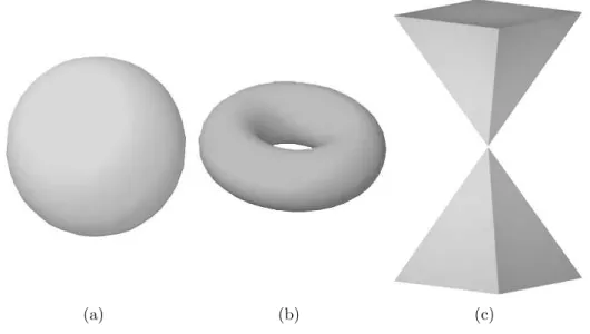
1.1 Sphere (a) and torus (b) are manifold surfaces. The connection of two triangular prisms as seen in (c), creates a non-manifold surface. Sphere has no hole so it is a genus-0 surface, while torus has one hole so it is a genus-1 surface. All the objects have one

shell. . . 5

1.2 A triangle strip created from a mesh. . . 13

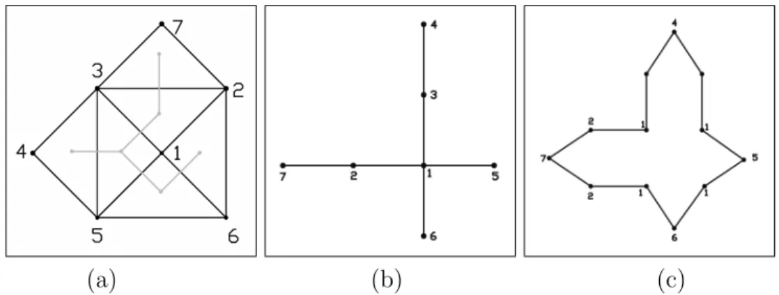
1.3 Spanning trees in the triangular mesh strip method. (a) Triangle spanning tree, (b) vertex spannig tree, (c) vertex spanning tree with doubled edge. . . 14

1.4 Opcodes defined in the EdgeBreaker. . . 15

1.5 Encoding example for EdgeBreaker. . . 15

1.6 Decoding example for EdgeBreaker. . . 16

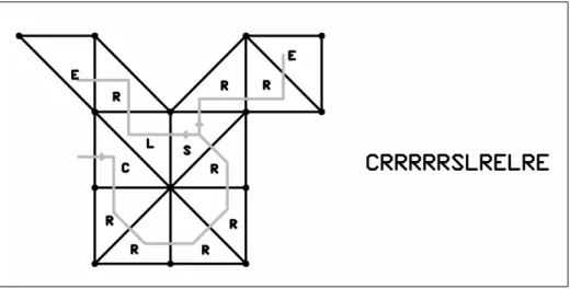
1.7 TG Encoding of the same mesh as EdgeBreaker. The resulting codeword will be [ 8,6,6,4,4,4,4,4,6,4,5,Dummy 13,3,3 ]. . . 18

1.8 The delta-coordinates quantization to 5 bits/coordinate (left) in-troduces low-frequency errors to the geometry, whereas Cartesian coordinates quantization to 11 bits/coordinate (right) introduces noticeable high-frequency errors. The upper row shows the quan-tized model and the bottom row uses color to visualize correspond-ing quantization errors. (Reprinted from [31] with courtesy of Dr. Olga Sorkine) . . . 20

1.9 Linear prediction. . . 21

1.10 Parallelogram prediction. . . 22

1.11 (a) A simple mesh matrix; (b) its valence matrix; and (c) its ad-jacency matrix. . . 23

1.12 Geometry images. (a) The original model. (b) Cut on the mesh model. (c) Parameterized mesh model. (d) Geometry image of the original model. (Reprinted from [5]Data Courtesy Hugues Hoppe) 25

1.13 Edge collapse and vertex split operations are inverse of each other. 27

1.14 Progressive representation of the cow mesh model. The model re-constructed using (a) 296, (b) 586, (c) 1738, (d) 2924,and (e) 5804 vertices. . . 28

1.15 Progressive forest split. (a) initial mesh; (b) group of splits; (c) remeshed region and the final mesh. . . 29

1.16 Valence based progressive compression approach. . . 30

2.1 (a) 2D rectangular sampling lattice and 2D rectangular sampling matrix. (b) 2D quincunx sampling lattice and 2D quincunx sam-pling matrix. . . 38

2.2 The illustration of the projection operation and the resulting

image-like representation. . . 39

2.3 Projected vertex positions of the mesh; (a) projected on XY plane; (b) projected on XZ plane. . . 40

2.4 (a) Original image (b) 4-level wavelet transformed image. . . 43

2.5 Lazy filterbank. . . 44

2.6 (a) The relation between wavelet coefficients in EZW; (b) the tree structure of EZW; (c) the scan structure of wavelet coefficients in EZW. . . 45

2.7 1D lifting scheme without update stage. . . 48

2.8 Lazy filterbank. . . 50

2.9 The block diagram of the proposed algorithm. . . 52

3.1 Reconstructed sandal meshes using parameters (a) lazy wavelet, 60% of bitstream, detail level=3; (b) lazy wavelet, 60% of bitstream, de-tail level=4.5; (c) Haar wavelet, 60% of bitstream, dede-tail level=3; (d) Daubechies-10, 60% of bitstream, detail level=3. (Sandal model data is from Viewpoint Data Laboratories) . . . 63

3.2 Meshes reconstructed with a detail level of 3 and 0.6 of the bit-stream. (a) Lazy, (b) Haar, (c) Daubechies-4, (d) Biorthogonal4.4, and (e) Daubechies-10 wavelet bases are used. . . 64

3.3 Homer Simpson model compressed with JPEG2000 to 6.58 KB (10.7 bpv). (a) The histogram of the error on the original model. (b) The original model. Color levels indicate the distortion be-tween the original and the reconstructed model. Blue is the lowest distortion level. As the distortion increases the color index goes from blue to green and then red. Red is the highest distortion level. (c) The reconstructed model. . . 67

3.4 Homer Simpson model compressed with JPEG2000 to 6.27 KB (10.1 bpv). . . 68

3.5 Homer Simpson model compressed with JPEG2000 to 9.28 KB (15 bpv). . . 69

3.6 Homer Simpson model compressed with JPEG2000 to 12.7 KB (20.6 bpv). . . 70

3.7 Homer Simpson model compressed with SPIHT to 4.07 KB (6.6 bpv). . . 71

3.8 Homer Simpson model compressed with SPIHT to 4.37 KB (7.1 bpv). . . 72

3.9 Homer Simpson model compressed with SPIHT to 4.67 KB (7.6 bpv). . . 73

3.10 Homer Simpson model compressed with SPIHT to 4.96 KB (8 bpv). 74

3.11 Homer Simpson model compressed with SPIHT to 5550 KB (9 bpv). 75

3.12 Homer Simpson model compressed with SPIHT to 6.76 KB (11 bpv). 76

3.14 The qualitative comparison of the meshes reconstructed without adaptive prediction (a and c) and with adaptive prediction (b and d). Lazy wavelet basis is used. The meshes are reconstructed us-ing 60% of the bitstream with detail level=5 in the Lamp model and 60% of the bitstream with detail level=5 in the Dragon model. (Lamp and Dragon models are courtesy of Viewpoint Data Labo-ratories) . . . 81

3.15 Distortion measure between original (images at left side of the fig-ures) and reconstructed Homer Simpson mesh models using Mesh-Tool [68] software. (a) SPIHT at 6.5 bpv; (b) SPIHT at 11 bpv; (c) JPEG2000 at 10.5 bpv. The grayscale colors on the original image show the distortion level of the reconstructed model. Darker colors mean more distortion. . . 82

3.16 Comparison of our reconstruction method with Garland’s simpli-fication algorithm [46] (a) Original mesh; (b) simplified mesh us-ing [46] (the simplified mesh contains 25% of the faces in the orig-inal mesh); (c) mesh reconstructed by using our algorithm using 60% of the bitstream. . . 83

3.17 (a) Base mesh of Bunny model composed by PGC algorithm (230 faces); (b) Model reconstructed from 5% of the compressed stream (69, 967 faces); (c) Model reconstructed from 15% of the compressed stream (84, 889 faces); (d) Model reconstructed from 50% of the compressed stream (117, 880 faces); (e) Model re-constructed from 5% of the compressed stream (209, 220 faces); (f) Original Bunny mesh model (235, 520 faces). The original model has a size of 6 MB and the compressed full stream has a size of 37.7 KB. . . 84

3.18 Homer and 9 Handle Torus models compressed using MPEG-3DGC. The compressed data sizes are 41.8 KB and 82.8 KB re-spectively. Figures on the left side show the error of the recon-structed model with respect to the original one. Reconrecon-structed models are shown on the right side. . . 85

3.19 The error between the original dancing human model and recon-structed dancing human models compressed using SPIHT 13.7 bpv (a) and 9.7bpv (c) respectively. (b) and (d) show the reconstructed models. The error between the original dancing human model and reconstructed dancing human models compressed using MPEG-3DGC at 63 bpv (e). (f) the reconstructed models. . . 86

3.20 (a) Dragon (5213 vertices) and (c) Sandal (2636 vertices) models compressed using MPEG-3DGC. (b) Dragon (5213 vertices) and (d) Sandal (2636 vertices) models compressed using The proposed SPIHT coder. Compressed data size are 43.1 KB and 10.4 KB, respectively for Dragon model and 22.7 KB and 2.77 KB respec-tively for Sandal model. . . 87

3.21 9 Handle Torus model compressed with JPEG2000 to 14.6 KB (12.4 bpv). (a) The histogram of the error on the original model. (b) The original model. Color levels indicate the distortion be-tween the original and the reconstructed model. Blue is the lowest distortion level. As the distortion increases the color index goes from blue to green and then red. Red is the highest distortion level. (c) The reconstructed model. . . 88

3.22 9 Handle Torus model compressed with JPEG2000 to 13.6 KB (11.6 bpv). . . 89

3.23 9 Handle Torus model compressed with JPEG2000 to 14 KB (11.9 bpv). . . 90

3.24 9 Handle Torus model compressed with JPEG2000 to 16.7 KB (14.2 bpv). . . 91

3.25 9 Handle Torus model compressed with SPIHT to 7.84 KB (6.7 bpv). 92

3.26 9 Handle Torus model compressed with SPIHT to 8.18 KB (7 bpv). 93

3.27 9 Handle Torus model compressed with SPIHT to 8960 KB (7.63 bpv). . . 94

3.28 9 Handle Torus model compressed with SPIHT to 11.9 KB (10.1 bpv). . . 95

3.29 9 Handle Torus model compressed with SPIHT to 12.7 KB (10.8 bpv). . . 96

List of Tables

3.1 Compression results for the single rate mesh connectivity coders in literature. . . 58

3.2 Compression results for the single rate mesh geometry coders in literature. . . 59

3.3 Compression results for the progressive mesh coder in literature (Geometry + Connectivity). . . 60

3.4 Compression results for the Sandal model. The Bitstream Used parameter shows how much of the encoded bitstream is used in the reconstruction of the original model. The Detail Level parameter defines the closeness of the grid points on the projection image (size of the projection image). As the Detail level increases the grid points of the projection plane gets closer (the projection image gets larger). . . 61

3.5 Comparative compression results for the Cow model compressed without prediction and with adaptive prediction. The Bitstream

Used parameter shows how much of the encoded bitstream is used

in the reconstruction of the original model. The Detail Level pa-rameter defines the closeness of the grid points on the projection image (size of the projection image). As the Detail level increases the grid points of the projection plane gets closer (the projection image gets larger). . . 62

3.6 Compression results for the Lamp model using lazy wavelet fil-terbank. The Bitstream Used parameter shows how much of the encoded bitstream is used in the reconstruction of the original model. The Detail Level parameter defines the closeness of the grid points on the projection image (size of the projection image). As the Detail level increases the grid points of the projection plane gets closer (the projection image gets larger). . . 65

3.7 Compression results for the Homer Simpson model using SPIHT and JPEG2000. Hausdorff distances are measured between the original and reconstructed meshes. . . 65

3.8 Compression results for the 9 Handle Torus mesh model using SPIHT and JPEG2000. Hausdorff distances are measured between the original and reconstructed meshes. . . 65

3.9 Comparative results for the Homer,9 Handle Torus, Sandal, Dragon, Dance mesh models compressed using MPEG-3DGC and SPIHT based mesh coder. SPIHT based mesh coder results in-cludes connectivity coding using EdgeBreaker. Hausdorff distances are measured between the original and reconstructed meshes. . . . 80

Chapter 1

Introduction

The demand to visualize the real world scenes in digital environments and make simulations using those data increased in last years. Three-dimensional (3D) meshes are used for representing 3D objects. The mesh representations of 3D objects are created either manually or by using 3D scanning and acquisition tech-niques [1]. Meshes with arbitrary topology can be created using these methods. The 3D geometric data is generally represented by two tables: a vertex list stor-ing the 3D coordinates of vertices and a polygon list storstor-ing the connectivity of the vertices. The polygon list contains pointers into the vertex list.

Multiresolution representations can be defined for 3D meshes [2]. In a fine resolution version of an object, more vertices and polygons are used as com-pared to a coarse representation of the object. It would be desirable to obtain the coarse representation from the fine representation using computationally ef-ficient algorithms. Wavelet-based approaches are applied to meshes to realize a multiresolution representation of a given 3D object [2].

As the scenes and the objects composing those scenes become more complex and detailed, the size of the data also grows. Therefore, the problem of transmit-ting this data from one place to another becomes a more difficult and important

task. The transmission can be over a band limited channel, either from one system to another system or from a storage device to processing unit e.g. from

main memory to graphics card [3].

“The fundamental problem in communication is that of reproducing at one point either exactly or approximately a message selected at another point” [4]. However the choice of the message data is not unique. There exists several pos-sible sets of messages that can be used to describe the transmitted information. The problem is to create a description that expresses the data best with the smallest size.

There exists several mesh compression approaches in the literature. Most of those approaches treats the meshes as 3D graphs in the space. The geometry and the connectivity data is compressed separately. The geometry images tech-nique explained in [5] compresses the meshes using image compression methods. The meshes are parameterized to two dimensional (2D) planes. Those param-eterizations of meshes are treated as images and compressed using any wavelet based image coder. Parameterization of a surface mesh is a complex task to be applied to an arbitrary object because many linear equations need to be solved. As the objects get more complex, parameterization becomes nearly impossible. The surfaces are cut for reducing the complexity of parameterization [6]. The adaptation of signal processing algorithms [7] to surface meshes is also a chal-lenging task although it is easier than parameterization. It is much easier to transform the data and apply any algorithm that is needed rather than adapting signal processing algorithms to 3D graphs.

These drawbacks in [5] gave us the idea of finding easier ways for mapping meshes to images and using image compression tools directly on those images. Since image processing is a well established branch of signal processing, there exists a wide spectrum of algorithms that can be used. Thus understanding of

the fundamentals behind compression especially image compression is an essential issue in our work.

1.1

Mesh Representation

3D Meshes are visualization of 3D objects using vertices (geometry), edges, faces, some attributes like surface normals, texture, color and connectivity. 3D points

{v1, ..., vn} ∈ V in R3 are called vertices of a 3D mesh. The convex hull of

two vertices in R3_{, conv{v}

n, vm} is called an edge. So an edge is mapped to

line segment in R3 _{with end points at v}

n and vm. Face of a triangular mesh

is a surface which is conv{vn, vm, vk}. Thus a face is mapped to a surface in

R3 _{that is enclosed by the edges incident to the vertices v}

n, vm, vk. A face may

have no direction or its direction can be determined using the surface normals data. The additional attributes of a mesh are mostly carried by the vertices. That information can be extended along the edges and the faces using linear interpolation or other techniques (e.g. linear, Phong shading of a surface).

The connectivity information summarizes which mesh elements are connected to each other. Edges {e1, ..., en} ∈ E are incident to its two end vertices. Faces

{f1, ..., fn} ∈ F are surrounded by its composing edges and incident to all the

vertices of its incident edges. The edges have no direction. Two types of mesh connectivity are common in mesh representations. Edge Connectivity is the list of edges in the mesh and Face Connectivity list of faces in the mesh. In a triangular mesh, since all the vertices of a face lie in a plane, the face also lies in a plane. In polygonal meshes the number of the vertices that are incident to the face, is four or more. So face of a polygonal mesh not necessarily lie in a plane.

Vertices of a mesh can be incident to any number of edges. The number of the edges that are incident to a vertex is called the valence of the vertex [8]. The number of the edges that are incident to a face is called the degree of a face [8].

The number of faces incident to an edge and the number of face loops incident to a vertex, are important concepts while defining, if the mesh is manifold or non-manifold. “A 2-manifold is a topological surface where every point on the surface has a neighborhood topologically equivalent to an open disk of R2_{” [9]. If the}

neighborhood of a point on the surface is equivalent to an half disk then the mesh is manifold with boundary [9]. In Figure 1.1 examples of manifold, manifold with boundary and non-manifold surfaces can be seen.

(a) (b) (c)

Figure 1.1: Sphere (a) and torus (b) are manifold surfaces. The connection of two triangular prisms as seen in (c), creates a non-manifold surface. Sphere has no hole so it is a genus-0 surface, while torus has one hole so it is a genus-1 surface. All the objects have one shell.

Two other important concepts about meshes are shell and genus. Shell is a part of the mesh that is edge-connected. The genus of a mesh is an integer that can be derived from the number of closed curves that can be drawn on the mesh without dividing it into two or more separate pieces. It is equal to the number of handles on the mesh object [8]. As seen in Figure 1.1(b) a torus is genus-1 since it has one hole and a sphere Figure 1.1(a) is genus-0 since it has no hole [8].

Connectivity of a mesh is a quadruple (V, E, F, Q) where Q is the incidence relation [9]. Relationships between mesh elements can be found using the con-nectivity information in Euler equation [8]. The Euler characteristics κ of a mesh can be calculated using,

κ = v − e + f , (1.1)

where v, e, f are the number of vertices, edges and the faces of a mesh respectively. The Euler characteristics of a mesh depends on the number of shells, genus and boundaries of the mesh. For closed and manifold meshes, the Euler characteristic is given as :

κ = 2(s − g), (1.2)

where s is the number of the shells and g is the genus number.

Simple meshes are meshes that are homeomorphic to a sphere which means they are topologically the same. Homeomorphism is a function between two spaces which satisfies the conditions of having bijection, being continuous and having a continuous inverse [10]. In other words, homeomorphism is a continuous stretching and bending of the mesh into a new shape.

Each triangle of a simple mesh has three edges and each edge is adjacent to two triangles. This leads us to :

2e = 3f . (1.3)

v − e + f = 2, (1.4) v − 1 2f = 2 , (1.5) v f = 2 f + 1 2 . (1.6)

For large meshes the assumption of Equation 1.7 can be made. Considering that each edge is connected to its two end vertices, the average valence for large, simple meshes can be calculated by averaging the sum of the valence, vali, of

each individual vertex vi where i ∈ Z, as,

f = 2v and e = 3v , (1.7) 1 v v X i = 1 vali ≈ 2e v = 6 . (1.8)

Basically a mesh is a pair M = (C, G) where C represents the mesh connec-tivity information and G represents the geometry information (3D coordinates). Connectivity information is closely related with the mesh elements whose ad-jacency and incidence informations are important for navigating in the mesh. Different mesh manipulation and compression algorithms depend on different properties of the mesh. Therefore, it is essential to represent the mesh in an appropriate way so that it can be easily used by those algorithms.

For instance, a connectivity compression algorithm EdgeBreaker [11], tra-verses faces of the mesh to encode the connectivity data of the mesh. Therefore, usage of a data structure, which enables easy access to adjacency information of the mesh, would increase the speed of the algorithm. Thus choosing an ap-propriate data structure that can be used with the chosen algorithm is also an important performance issue. Different edge based data structures such as

1.2

Compression

Compression is the selection of a more convenient description for transmitting the information using the smallest data size. For lossless transmission the best that can be done is to reach a near entropy bit-rate. For lossy transmission the situation is more complex. For different distortion levels of the data, different entropies can be found. Thus different lower bounds for data compression exist. The goal is to transmit the smallest amount of information by which the original data can be reconstructed in the predefined distortion bounds.

Mostly data and information are confused with each other. Data is the means by which the information is conveyed. However various data sizes can be used to transmit the same amount of information. It is just like two person describing the same scene in two different ways. One may tell it is a “forest” and the other may tell “several trees enumerated near each other”. Data compression is the process of reducing the data size required to represent a given quantity of information [15]. For example a 256 color leveled 1024 x 1024 sized image which has independent uniformly distributed pixel color values, would require a data size of 8 MB. However, if the image is known to have a constant color, it can be compressed to 3.5 Bytes: 1 Byte for its color information and 2.5 Bytes for the images size information instead of 8 MB. For this image, the remaining data restates the already known facts that can be named as data redundancy.

1.2.1

Compression and Redundancy

There exist several types of redundancies for different types of data. For ex-ample in digital image compression, three basic types of redundancy are coding,

interpixel and pyschovisual redundancy. For the proposed 2D representations of

its place to redundancies between vertex positions (geometry information) and connectivity.

Explanation of coding redundancy comes from the probability theory. If a symbol is more probable than another one, it should be represented using less number of bits. Histograms are very useful for this purpose since they show how many times a value is taken in the data. Normalized versions of histograms with infinite number of samples converges to probability density functions with the ergodicity assumption. So histograms with finite number of samples give a very good insight about the probability of a specific symbol. Probability of each level in an L color image with n pixel is,

p(k) = nk

n , k = 0, 1, ..., L − 1 , (1.9)

where nkis the number of times that kthcolor level appears in the image, and n is

the number of image pixels. The Average Code Length (ACL) can be calculated using, ACL = L−1 X k=0 l(k)p(k) , (1.10) where l(k) is the code length of the level k.

To minimize the total code length, average code length must be minimized. Using different symbol code lengths and giving shorter codes to the symbols with higher probability will minimize the average code length.

Lower variance in the histogram leads to better compression since the data is more predictable. The histogram of a single colored image has only one value at one specific color level so the whole data can be predicted from that pixel very well. Another example can be compression of sentences in English. The

’e’ letter is the most frequently used letter in English so assigning ’e’ a shorter

symbol than the other letters, gives us smaller encoded data size.

Pyschovisual redundancy comes from the imperfection of the human visual system. The difference between the positions of two points can not be perceived after some distance. So quantizing coordinates of points in 3D space do not change the visualization of the data.

In images most of the neighboring pixels are not independent from each other. This means there is a correlation between them. At the low frequency parts of the image this correlation is even more stronger. This is also true for meshes. However, the situation is a little bit different. The neighboring concept is de-pendent on not only being near to each other but also being connected to each other. Connected pixels can be predicted from each other more reliably. The correlation between the vertices at the smooth regions of the 3D mesh is stronger like the correlation between the pixels in the low pass parts of the images.

1.3

Related Work on Mesh Compression

There are several mesh compression algorithms in the literature [16, 8, 47]. They can be classified as single-rate compression and progressive mesh compression. This classification can be further extended to sub groups called, connectivity and

geometry compression. In most of the algorithms the connectivity information is

exploited for more efficiently compressing the geometry information of the mesh.

Compression is not the only way of reducing the size of a mesh. Methods like simplification and remeshing are also used for this purpose. In this section those concepts will also be mentioned in the context of compression. The aim of mesh compression is to transmit a mesh from one place to another using as small information as possible. To achieve this aim, connectivity is encoded in a

lossless manner and geometry is encoded in either lossless or lossy manner. Due to the quantization of the 3D positions of the vertex points, most of the geometry encoders are lossy.

Remeshing is a popular method for converting an irregular mesh to a semi-regular or semi-regular mesh. The idea in remeshing is to represent the same object with more correlated connectivity and vertex position information while causing the least distortion. This makes the new mesh more compressible since many of the vertices can be predicted from its neighbors. It can be thought of as regularizing the mesh data. However, remeshing is a complex task.

Single rate encoders compress the whole mesh into a single bit stream. The encoded connectivity and the geometry streams are meaningless unless the whole stream is received by the decoder. In the context of single rate encoders, there exists several algorithms like, triangle strip coding [3], topological surgery [17], EdgeBreaker [11], TG coder [18], valence-based coder of Alliez and Desbrun [16], Spectral coding [19], geometry images [5]. They are also used in compression of the base meshes of progressive representation. Single rate mesh compression will be dealt in more detail at 1.3.1

Progressive compression has the advantage of representing the mesh at multi-ple detail levels. A simplified version of the original model can be reconstructed from some initial chunks of coded stream. The remaining chunks will add refine-ments to the reconstructed model This is an important opportunity for environ-ments like Internet or scenes with multiple meshes where impression of existence of the object is more important then its details.

Progressive mesh representations [20] store a 3D object as a coarse mesh and a set of vertex split operations that can be used to obtain the original mesh. Pro-gressive mesh representations use simplification techniques such as edge collapse

and vertex removal to obtain the coarser versions of the original mesh. Subdivi-sion technique can also be regarded as a progressive mesh representation [21, 33]. In [23, 2], multiresolution approaches for mesh compression using wavelets are developed. Progressive mesh compression will be dealt in more detail at 1.3.2

Besides static meshes, there exists animation of meshes called dynamic meshes. Some of the static and progressive mesh compression algorithms are used for encoding them. Besides intra-mesh redundancies, those mesh sequences have inter-mesh redundancies. Each mesh can be thought as a frame of an animation and the redundancies between frames should be exploited for more efficiently compressing dynamic meshes. Several algorithms like, Dynapack [24], D3DMC [25, 26], RD-D3DMC [27, 26] exists for encoding dynamic meshes.

Uncompressed mesh data is large in size and contains redundant information. Each triangle is specified by three vertices which are 3D points in R3 _{and some}

attributes like surface normals,color,etc. If the vertex coordinates are quantized to 4 byte floating point values, a vertex needs 12 bytes only for its geometry information. From Equation 1.8 it is known, that each vertex is connected to 6 triangles. If a triangle is represented by the data of its three vertices, each vertex would be transmitted 6 times. This means a data flow of 72 bytes per vertex. To decrease this data flow, more efficient representations of the mesh should be used. Encoding the mesh is one of the best way of reducing this data flow.

1.3.1

Single Rate Compression

A 3D mesh model is basically composed of two data namely, Connectivity

infor-mation and Geometry inforinfor-mation. So two types of compression for those two

Connectivity Compression

In the connectivity information each vertex is six times repeated in average. One simple way to reduce the number of vertex transmission is creating triangular strips from the mesh as in Figure 1.2. In this method, the initial triangle is described using its three vertices. The next triangle which is a neighbor of the current one, will be formed using the two vertices from the joined edge and a new vertex. So for each triangle of the strip, one vertex will be transmitted. From Equation 1.7 it is known that in the large simple meshes there exist twice as many faces as the vertices. So if triangle strip method is used, each vertex will be transmitted twice.

Figure 1.2: A triangle strip created from a mesh.

Deering [3] proposed an idea of using a vertex buffer to store some of the transmitted vertices in order not to transmit each vertex twice. The new triangle in the strip either introduces a new vertex which will be pushed in the vertex buffer or a reference to the vertex buffer. This gives the algorithm the advantage of re-using the transmitted vertices.

For achieving this, Deering proposed a new mesh representation called

gen-eralized triangle mesh. The mesh is converted into an efficient linear so that

the geometry can be extracted by a single monotonic scan over the vertex ar-ray. However, references to the used vertices are inevitable. Buffering solves the problem to some extend. Deering used a vertex buffer with size 16 in [3].

A triangle strip is a part of triangle spanning tree (Figure 1.3(a)), whose nodes are the faces of the mesh and edges are the adjacent edges of the mesh faces. This is the dual of the connectivity graph, whose nodes are the vertices (Figure 1.3(b)) and edges are the edges of the mesh. Taubin proposed Topological Surgery [17] algorithm to encode the connectivity of a mesh using those two trees. Both the triangle and the vertex spanning trees are encoded and sent to the receiver. The decoder at the receiver side first decompresses the vertex spanning tree and doubles each of its edges (Figure 1.3(c)). After decoding the triangle spanning tree the resulting triangles are inserted between pairs of doubled edges of the vertex spanning tree.

(a) (b) (c)

Figure 1.3: Spanning trees in the triangular mesh strip method. (a) Triangle spanning tree, (b) vertex spannig tree, (c) vertex spanning tree with doubled edge.

Region growing is another approach for connectivity compression. Rossignac’s EdgeBreaker [11] is one of the examples for this approach. In [11] a region growing starting with a single triangle is done. The grown region contains the processed triangles. The edges between the processed and to be processed region is called the cut-border. A selected edge in the cut border, which defines the next processed

triangle, is called the gate.

Each next triangle can have five different possible orientations with respect to the gate and cut-border. Each orientation has its own opcode. By this way each processed triangle is associated with an opcode. This iterative process goes

Figure 1.4: Opcodes defined in the EdgeBreaker.

on until no unprocessed triangles left in the mesh. Those mentioned elements can be seen in Figure 1.4.

Figure 1.5: Encoding example for EdgeBreaker.

Since the decoder knows how the mesh connectivity is encoded, it can recon-struct the mesh connectivity by inverting the operations done by the encoder. Figure 1.6 shows decoding of the mesh in Figure 1.5. Split operation is a special occasion while decoding. Each split operation has an associated end operation which finishes the cut-border introduced by the split operation. The length of each run starting with a split is needed while decoding the symbol array. There-fore, EdgeBreaker needs two runs over the symbol array.

This problem is solved by Wrap&Zip [28] and Spiral Reversi [29] which are extensions on EdgeBreaker. Wrap&Zip solves the problem by creating dummy vertices for split operations while encoding the mesh (wrap) and identifying them in the decoding phase (zip). Spiral Reversi decodes the symbol stream starting

Figure 1.6: Decoding example for EdgeBreaker.

from the end. By this way the decoder first finds the end opcodes and then associated split opcodes.

In [18], Touman and Gotsman also introduced a region growing algorithm. But instead of coding the relation between gates and the triangles, they code the valences of the processed vertices. If the variance of the valences of the mesh vertices is small, the mesh connectivity can be compressed efficiently. From Eq. 1.8 we know that, vertices of large meshes have an average valence of six. Also by remeshing, irregular meshes can be converted into semi-regular or regular meshes whose valences are mostly six. So this method is very efficient on regular and semi-regular meshes.

The TG coder first connects all the boundary vertices of the mesh with a dummy vertex as seen in Figure 1.7. Instead of selecting a starting triangle like EdgeBreaker, TG coder selects a starting vertex and outputs its valence with two other vertices of a triangle incident to the starting vertex. The triangle is

marked as conquered and its edges are added to the cut-border. The conquest of the incident triangles are iterated counter-clockwise around the focus vertex. When all the triangles incident to the focus vertex are conquered, the focus moves to the next vertex along the cut-border. This iterates until all the triangles are conquered. If dummy vertex becomes the focus vertex, the special symbol for dummy is output together with the valence of the dummy vertex.

Figure 1.7: TG Encoding of the same mesh as EdgeBreaker. The resulting codeword will be [ 8,6,6,4,4,4,4,4,6,4,5,Dummy 13,3,3 ].

A split situation can occur in this algorithm, too. It can arise when the cut-border is split into two parts. In this situation one of the cut-cut-borders is pushed into the stack. The number of edges along the cut-border must also be encoded.

The split situation is an unwanted event since it complicates the encoding process. To reduce the number of the split situations, in [16] Alliez and Desbrun proposed an improved version of the TG coder. They approach the problem with the assumption of, “split situations are tend to arise in convex regions”. So it is more reasonable to select focus vertices from concave regions instead of convex regions. While choosing the focus vertices, the algorithms pay attention to how

many free edges the vertex neighbors. The vertex with minimum free edges is chosen. If there exists a tie between two vertices, number of the free edges of their neighbors will be taken into account.

Geometry Compression

The geometry data has a floating point representation. Due to the limitations of the human visual perception, this representation can be restricted to some precision which is called quantization. Nearly for all the mesh geometry codes, quantization is the first step of compression. The early works uniformly quantize each coordinate value separately in Cartesian plane. Moreover, vector quan-tization of the mesh geometry is proposed in [30]. Karni and Gotsman also demonstrated the need for applying quantization on spectral coefficients [19] .

Sorkine et al. proposed a solution to the problem of minimizing the distortion in visual effects due to the quantization [31]. They quantize the vertices that are on the smooth parts of the mesh more aggressively. The basis behind this idea is the fact that human visual system is more sensitive to distortion in normals than geometric distortion. Therefore, they try to preserve the normal variations over the surfaces. In Figure 1.8 an illustrative comparison between quantization in Cartesian coordinates and delta-coordinates can be seen.

The prediction of the quantized vertices is a commonly used technique in mesh compression. To predict pixels from their neighbors is a well known tech-nique in image processing. In some sense, the same approach is used in mesh compression. While traversing the mesh, position of the vertices are predicted from the formerly processed vertices. The prediction error, which is the difference between the predicted position and the real position, is coded. The prediction errors tend to converge around a mean value with a small variance.

Figure 1.8: The delta-coordinates quantization to 5 bits/coordinate (left) in-troduces low-frequency errors to the geometry, whereas Cartesian coordinates quantization to 11 bits/coordinate (right) introduces noticeable high-frequency errors. The upper row shows the quantized model and the bottom row uses color to visualize corresponding quantization errors. (Reprinted from [31] with courtesy of Dr. Olga Sorkine)

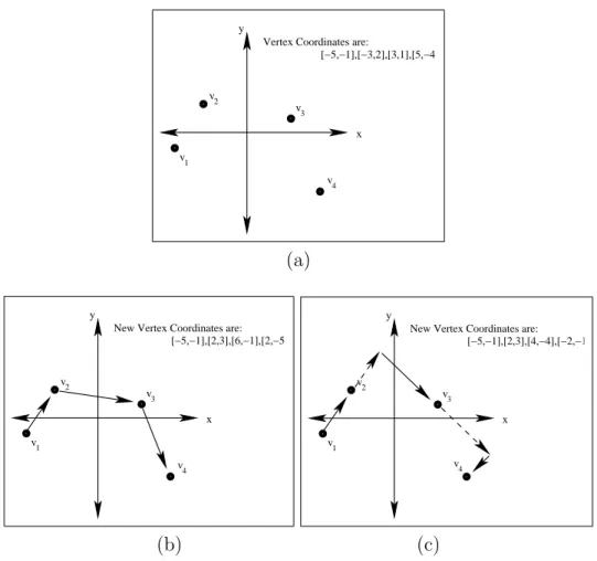
There exist several schemes to predict the vertex positions. The most known ones are: linear prediction using the weighted sum of the previous vertices (in the order given by the connectivity coder) as shown in Figure 1.9, parallelogram prediction as shown in Figure 1.10, and multi-way prediction as in [32].

Touma and Gotsman introduced the Parallelogram prediction together with their TG coder [18]. This type of prediction is currently one of the most popular one. The basis of the idea is that, each edge has two incident triangles. So the position of a vertex v4 can be predicted using the vertices of the neighboring

triangle, v1, v2, v3 with respect to the opposing edge of v4. Vertices v2, v3 also

v₂

v₁

v₃

Vertex Coordinates are: y x [−5,−1],[−3,2],[3,1],[5,−4] v₄ (a) v₂ v₁ v₃

New Vertex Coordinates are: y x [−5,−1],[2,3],[6,−1],[2,−5] v₄ v₂ v₁ v₃

New Vertex Coordinates are: [−5,−1],[2,3],[4,−4],[−2,−1] y

x

v₄

(b) (c)

Figure 1.9: Linear prediction.

gives an illustration of parallelogram prediction algorithm. The vertex v4 is

predicted using

ˆ

v4 = v2+ v3− v1 , (1.11)

and the error can simply be found by subtracting the predicted value from the actual position as,

e = ˆv4− v4 . (1.12)

In linear and parallelogram prediction schemes the vertex is predicted from one direction. This kind of prediction is not efficient for meshes with creases and corners. In [32] a prediction scheme, which uses the neighborhood information

e

3

v

2

v

v

4

v

₁

v

4

^

Figure 1.10: Parallelogram prediction.

of the vertices to make predictions of the vertex positions, is proposed. In that scheme a vertex is predicted from all of its connected neighbors. The connected neighbors of a vertex can be found using the connectivity information of the mesh.

Another approach in geometry compression is adapting the idea of spectral coding [19] to 3D signals so they can be used in compression of meshes. The idea is finding the best representatives for the mesh and code them. It is similar to transforming an image into another domain and take the parts that has the most information. A known example of this kind of coding is DCT or wavelet coding of the images. More attention is paid to the low frequency parts since they represent the image much better than the high frequency parts . Using the same convention, basis functions that represents the signal best are found.

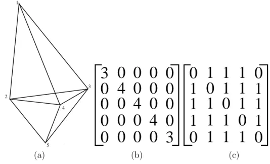
The eigenvectors of the Laplacian matrix corresponds to the basis functions. The Laplacian L of a mesh is defined using diagonal valence matrix VL and adjacency matrix A. The Laplacian L can be calculated as,

L = VL − A , (1.13)

L = UDUT _{, (1.14)}

e

V = UTV . (1.15)

Figure 1.11 shows L, VL and A for a simple mesh.

2 5 3 4 1

0 0 0 0

3

4 0 0 0

0

0 4 0 0

0

0 0 4 0

0

0 0 0 3

0

1 1 0

0

1 1 1

1

1 0 1 1

1

1 1 0 1

1

1 1 1 0

0

1

0

(a) (b) (c)

Figure 1.11: (a) A simple mesh matrix; (b) its valence matrix; and (c) its adja-cency matrix.

Using Equation 1.14 eigenvectors of L can be evaluated. U contains the eigenvectors of L sorted with respect to their corresponding eigenvalues. The ge-ometry information is represented using a v by 3 matrix V where v is the number of the vertices of the mesh. V is projected into the new basis by Equation 1.15. The rows of eV that are corresponding to low eigenvalues. Thus they can be skipped and remaining coordinates can be encoded efficiently.

This representation also allows for progressive transmission. Important co-ordinates are encoded and sent first. Therefore, rows corresponding to smaller eigenvalues are encoded and sent first. A low resolution mesh can be recon-structed from the first stream. Then the mesh can be refined as the lower priority

However there exists a disadvantage of using spectral coding. For larger ma-trices, decomposition in Equation 1.14 runs into numerical instabilities because many eigenvalues tend to have similar values. Also in terms of computation time calculating Equation 1.14 becomes an expensive job as the mesh grows.

Not only spectral coding but also the other mesh coding algorithms sometimes can not handle massive datasets like the model of David of Michelangelo. Those datasets should be partitioned into small enough meshes called in-core, in order to be compressed efficiently. In [34] Ho et al proposed an algorithm that partitions the massive datasets into small pieces and encode them using EdgeBreaker and

TG. Also there is an overhead for stitching information exists. There exists a

25% increase with respect to the compression of the small sized meshes using the same tools. In [35] Isenburg and Gumbold made several improvements over [34] like avoiding to break the mesh, decoding the entire mesh in a single pass, streaming the entire mesh through main memory with a small memory foot-print. This is achieved by building new external memory data structures (the

out-of-core mesh) dedicated for clusters of faces or active traversal fronts which

can fit in this cores.

Besides cutting and stitching, some of the algorithms transform the meshes to other data structures and encode those new data structures. Formerly mentioned

Spectral coding and Geometry images [5] are examples to this type of algorithms.

The basic idea in [5], is finding a parameterization of the 3D mesh to a 2D image and use image coding tools to code this image. To parameterize the mesh, it is cut along some of its edges and becomes topologically equivalent to a disk. This is one of the most challenging task of the algorithm. Finding those cuts is not a straight-forward think to do.

Parameterization domain is the unit square (2 pixel by 2 pixel). The pixel values of the parameterized mesh correspond to points on the original mesh. Those points may either be vertex locations or surface points (points in triangular

(a) (b)

(c) (d)

Figure 1.12: Geometry images. (a) The original model. (b) Cut on the mesh model. (c) Parameterized mesh model. (d) Geometry image of the original model. (Reprinted from [5]Data Courtesy Hugues Hoppe)

faces.). X, Y, Z coordinates of the points are written to the RGB channels of the image (Figure 1.12). A normal map image, which defines all normals for the interior of a triangle, is stored too. A geometry image is decoded simply by drawing 2 triangles for each unit square and taking the RGB values as the 3D coordinates. Using the normal map the new mesh can be rendered. But the original mesh cannot be reconstructed. The decoded mesh will become like a remeshed version of the original one, not exactly the original.

Remeshing is the process of approximating the original mesh using a more regular structure. There exists 3 types of mesh in this sense : Irregular, semi-regular, regular meshes. Most of the algorithms in the literature are adapting to the uniformity and regularity of the meshes [36]. So converting meshes into regular structures will bring the opportunity for compressing the meshes more efficiently. For example valence-based compression approach in [16] codes regular meshes very efficiently since in a regular mesh most the vertices has a valence of 6.

But remeshing is a hard task to accomplish. In [37], Szymczak introduced an idea of partitioning the mesh and resampling the partitioned surface. The resampled surface is retriangulated by referencing the normals of the original mesh surface. Here both partitioning and retriangulation are computationally expensive and non-trivial tasks to do.

1.3.2

Progressive Compression

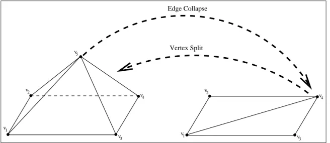
Lossless Compression Techniques

The basic idea behind Progressive Mesh (PM) compression is to simplify a mesh and record the simplification steps. So the simplification can be inverted using the recorded information. PM coding is first introduced by Hoppe in [20]. He defined operation called edge collapse and vertex split. Figure 1.13 illustrates these operations.

An edge collapse operation merges two vertices incident to the chosen edge and connects all the edges connected to those vertices to the merged vertex. The vertex split operation is the inverse of edge collapse. After a sequence of edge collapses, a simplified version of the original mesh is established (Figure 1.14(c)). One of the single rate coders can be used to encode this simplified mesh. The

v₂ v4 v₃ v₂ v₁ v₄ v₃ v₁ v₅ Vertex Split Edge Collapse

Figure 1.13: Edge collapse and vertex split operations are inverse of each other.

receiver side first decodes the simplified mesh and then uses the coming informa-tion to inverse the edge collapses by vertex split operainforma-tion. Merged vertices are separated and those new vertices are connected to their neighbors

The selection of the edge to be collapsed next is an important issue since it affects the distortion of the simplified mesh. Hoppe [20] uses an energy function which takes into account the distortion that will be created by collapsing the edge. An energy value is assigned to each vertex. Incrementally an edge queue is created by sorting those energy values. The selection of the next edge to be collapsed is done according to this queue.

The progressive simplicial complexes approach in [38] extends the PM algo-rithm [20] to non-manifold meshes. Popovic and Hoppe [38] observed that using edge collapses resulting in non-manifold points, gives a lower approximation er-ror for the coarse mesh. So they generalized the edge collapse method to vertex unification operation. Contrary to edge collapse, in vertex unification, the uni-fied two vertices may not be connected by an edge. Arbitrary two vertices from the mesh can be unified. Inverse operation is called generalized vertex split. The method can simplify arbitrary topology but has a higher bitrate than the PM

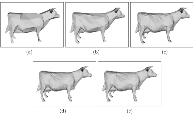
(a) (b) (c)

(d) (e)

Figure 1.14: Progressive representation of the cow mesh model. The model reconstructed using (a) 296, (b) 586, (c) 1738, (d) 2924,and (e) 5804 vertices.

algorithm since it has to record the connectivity of the region collapsed while unifying two vertices.

Another approach that is based on the PM method is introduced in [39] called

progressive forest split(PFS). Contrary to the PM method, between two

succes-sive levels of detail there exists a group of vertex splits in PFS. Due to the split of multiple vertices in the mesh, cavities may occur in the mesh. Such cavities are filled by triangulation. The positions of newly triangulated vertices are cor-rected using translations. So each PFS operation encodes the forest structure, triangulation information and vertex position transitions. The PFS method is part of the MPEG-4 version 2 standard.

Compressed progressive meshes (CPM) method introduced by Pajarola and

Rossignac is similar to the PFS method because it also refines the mesh using multiple vertex splits called batches. But contrary to the PFS method, in CPM method cavities do not occur. The vertices that will result in new triangles

after vertex split, are put in the batch. Thus connectivity compression is also easier in the CPM method,because no triangulation information is needed to be transmitted. Transition information in the PFS method is replaced with prediction information. Position of the new vertices are predicted from their neighbors using butterfly scheme.

(a) (b)

(c)

Figure 1.15: Progressive forest split. (a) initial mesh; (b) group of splits; (c) remeshed region and the final mesh.

Techniques mentioned so far are all the PM based approaches. Alliez and Desbrun proposed in [40] a method which uses the valence information of the vertices of the mesh. From Equation 1.8 it is known that average valence value of a mesh is 6. They observe that the entropy of the mesh is closely related

with the distribution of this valence. Their proposed algorithms has two parts:

decimation conquest and cleaning conquest.

Figure 1.16: Valence based progressive compression approach.

The decimation conquest first subdivides the mesh into patches. Each patch consists of triangles that are incident to a vertex as shown in Figure 1.16 (a). Then the encoder enters the patches one-by-one, removes the common vertices and re-triangulates the patch as shown in Figure 1.16(b-c). The valence of the removed vertex is output. This is applied to all of the patches in the mesh. Then, the cleaning conquest decimates the remaining vertices with valence 3. This algorithm preserves the average value around 6. The mesh geometry is encoded using barycentric prediction, and the prediction error is coded.

Lossy Compression Techniques

The basic idea behind lossy mesh compression is existence of another surface which is a good approximation of the original one and more capable for compres-sion. In lossy compression the original geometry and the connectivity informa-tion are lost. The distorinforma-tion between the original and its representative models is measured as the geometric distance between surfaces of those.

Multiresolution analysis and wavelets are the key methods in lossy mesh compression algorithms. They allow to decompose a complex surface into coarse representations together with refinements stored in the wavelet coefficients. Sur-face approximations at different distortions levels can be obtained by discarding or quantizing wavelet coefficient at some level. Since the mesh is decomposed into more energetic low frequency (multiresolution mesh levels) and low variance high frequency (wavelet coefficients) parts, a more compact compression can be achieved.

Wavelets are known as signal processing tools on Cartesian grids like audio, video, and image signals. Lounsberry et al. in [2] extended the wavelets to 2-manifold surfaces of arbitrary type. Due to their non-regularity, it is impossible to adapt wavelet transform to irregular meshes [41]. However, by creating semi-regular meshes using remeshing process, the mesh can be made semi-regular. On this regular structure an extension of the wavelet transform can be used.

The remeshing process is implemented by subdivision. The algorithm starts with the coarse representation of the original model called base mesh. Each triangle of the base mesh subdivided into 4 triangles by creating vertices on the edges of the face. The positions of those vertices represent again surface samples of the original model. So the subdivided coarse mesh becomes more and more similar to the original model. However, the new representation is a semi-regular mesh whose connectivity is regular.

After obtaining the semi-regular structure, the model is ready for progressive compression. The idea in multiresolution mesh analysis is to use wavelet trans-form between two resolution levels to code the prediction errors in the vertex locations. While going from the course to fine resolution the positions of the deleted vertices are predicted using subdivision. The difference, ve, between the

predicte, vp and the decimated vertex position, v, is stored as wavelet coefficients

as:

ve= vp− v , (1.16)

where v, ve, vp ∈ R3.

The process is similar to the high-pass filtering since the wavelet coefficients store the refinements of the mesh vertex positions. In the coarse to fine transition, first the vertex positions are predicted using subdivision and then repositioned using the wavelet coefficients. Discarding some of the wavelets to achieve better compression rates is possible. However, it is obvious that this brings distortion to the reconstructed model.

The third important part in progressive compression of the meshes is the coding of the base mesh and wavelet coefficients. As mentioned base mesh coding can be done using one of the single rate mesh coder. Wavelet coefficients are coded using entropy coders. Zero-tree coders would efficiently code this type of data since the coefficient tend to decrease from coarse to fine levels.

Khodakovsky in [42] proposed a lossy progressive mesh compression approach that uses MAPS [44] algorithm to remesh the original model to a semi-regular mesh. In [42] Loop scheme [33] is used to predict the vertex positions. In this algorithm the wavelet coefficients are 3D vectors as seen in Equation 1.16.

In [43] Khodokovsky and Guskov used normal meshes [22] and NMC wavelet coder to encode meshes. NMC coder uses normal meshes to encode the wavelet

coefficients. Wavelet coefficients are shown as scalar offsets (normals) in the perpendicular direction relative to the face. So wavelet coefficients become scalar values instead of 3D vectors. They used unlifted butterfly scheme [45] as predictor and it is also used while normal remeshing.

In [47] M´oran and Garcia proposed a method that generates the base mesh using Garland’s quadratic-mesh simplification [46]. They make predictions us-ing the butterfly scheme in [45]. The prediction errors are coded as wavelet coefficients. The normal component of the wavelet coefficients carry more infor-mation than the tangential components [47]. Thus wavelet coefficients are finely quantized in normal direction and coarsely quantized in tangential direction. A bit-wise interleaving of three detail components gives a scalar value so that a stream of scalar values is generated. This stream is coded using the SPIHT algorithm [48].

1.4

Contributions

This thesis proposes a framework to compress 3D models using image compres-sion based methods. In this thesis two methods are presented:

• a projection method to transform meshes into image objects,

• a connectivity based adaptive wavelet transformation (WT) scheme that

can be embedded into a known image coder and this WT scheme is used in the coding of image objects.

The proposed projection method is computationally easier than cutting and parameterizing the mesh as proposed in [5]. The proposed Connectivity-Guided Adaptive Wavelet Transform redefines the pixel neighborhoods. Thus it is more efficient than using ordinary wavelet transform schemes on the projection images

1.5

Outline of the Thesis

In the second chapter of this thesis, the proposed algorithm is explained in detail. The components of the algorithm include projection operation, Connectivity-Guided Adaptive Wavelet Transform, Set Partitioning in Hierarchical Trees (SPIHT), JPEG2000, map coding and reconstruction are explained. The main aim is to find a way to use image coders for mesh coding and embed adaptiveness to the image coder so that better bit rates can be achieved. In this thesis, this aim is achieved by using adaptive versions of the SPIHT and JPEG2000 image coders.

In the third chapter, mesh coding results of our algorithm and comparison with the algorithms in literature will be presented. Chapter 4 involves the con-clusions related to this thesis.

Chapter 2

Mesh Compression based on

Connectivity-Guided Adaptive

Wavelet Transform

This chapter is composed of several sections dealing with different parts of the mesh coding algorithm. These sections include mesh to image projection, Connectivity-Guided Adaptive Wavelet Transform, map coding and reconstruc-tion. The combination of all of those parts results in a complete mesh coder which can encode 3D models using any wavelet based image coders with minor modifications.

The proposed mesh coding algorithm introduces an easy way of converting meshes to image like representations so that 2D signal processing methods be-come directly applicable to a given mesh. After the projection, the mesh data becomes similar to an image whose pixel values are related to the respective coordinates of the vertex point to the projection plane.

The mesh data on a regular grid is transformed into wavelet domain using an adaptive wavelet transform. The idea of adaptive wavelets [49] is a well

known and proved to be a successful tool in image coding. Exploiting the di-rectional neighborhood information between pixels, adaptive wavelet transform beats its non-adaptive counterparts. Thus instead of using non-adaptive wavelet transform we come up with the idea of defining an adaptive scheme. Using the proposed adaptive scheme neighborhood information of the vertices can be better exploited.

2.1

3D Mesh Representation and Projection

onto 2D

A mesh can be considered as an irregularly sampled discrete signal. This means that the signal is only defined at vertex positions. In the proposed approach, the mesh is converted into a regularly sampled signal by putting a grid structure in space; corresponding to resampling the space with a known sampling matrix and quantization.

2.1.1

The 3D Mesh Representation

The 3D mesh data is formed by geometry and connectivity information. The geometry information of the mesh is constituted by vertices in R3_{. The}

3D-space, where the geometry information of the original mesh model is defined, is X0 _{= (x}0_{, y}0_{, z}0₎T _{∈ R}3_{. The vertices of the original 3D model are represented}

by v0

i = (x0i, yi0, z0i)T, i = 1, . . . , v where v is the number of the vertices in the

mesh.

First, the space that we use is normalized in R3_{[−0.5, 0.5] as,}

X = (x, y, z)T _{= αX}0_{, α = (α}

result in a normalization in the coordinates of the mesh vertices. The normalized mesh vertices are represented as,

vi = (xi, yi, zi)T = (αxx0i, αyy0i, αzzi0), i = 1, . . . , v . (2.2)

Connectivity information is represented as triplets of vertex indices. Each triplet corresponds to a face of the mesh. Faces of the mesh can be represented as,

Fi = (va, vb, vc)T, i = 1, . . . , f & a, b, c ∈ {1, . . . , v}, a 6= b 6= c , (2.3)

where f is the number of the faces and v is the number of the mesh. So a mesh in R3 _{can be represented as,}

M = (V, F) , (2.4)

where V is the set of vertices of the mesh and F is the set of faces of the mesh.

2.1.2

Projection and Image-like Mesh Representation

The 3D mesh representation is transformed into a 2D image-like representation by projecting the mesh data onto a plane. In this thesis a projection is defined as the transformation of points and lines in one plane onto another plane by connecting corresponding points on the two planes with parallel lines [52]. This is called Orthographic projection. The points of projection in our algorithm are vertices of the mesh. The selected projection plane is defined as P(u, w). The projection plane, P, is discritized using the sampling matrix, S. Different sampling matrices which are illustrated in Figure 2.1, can be defined as,

Srect =   T 0 0 T   _{, (2.5)}

for rectangular sampling and

Squinc =   T T /2 0 T /2   _{, (2.6)}

for quincunx sampling.

n 2 (t, t)

...

...

n 1

T 0

0 T

(

)

rect

S =

(a) n 2 n 1 (t/2, t/2)

...

...

T T/2

0 T/2

(

)

quinc

S =

(b)

Figure 2.1: (a) 2D rectangular sampling lattice and 2D rectangular sampling matrix. (b) 2D quincunx sampling lattice and 2D quincunx sampling matrix.

Due to its shape quincunx sampling lattice makes better approximations of the projected mesh vertices. But implementation of the rectangular is more straight-forward and computationally easy. After the projection operation, grid points, which are sampled using quincunx sampling lattice, must be transformed to a rectangular arrangement because the pixels of the image-like representation lined up in a rectangular manner. The projection of a 3D mesh structure mainly depends on two parameters of the vertex: Coordinates of the vertex and the perpendicular distance of the vertex to the selected projection plane.

Let ˇvi, which is a 2D vector, be the projection of vionto the plane P.