Geometric computing and
uniform grid technique
V Akman, W R Franklin*, M Kankanhalli* and C Narayanaswami
If computational geometry should play an important role in the professional environment (e.g. graphics and robotics), the data structures it advocates should be readily implementable and the algorithms efficient. In the paper, the uniform grid and a diverse set of geometric algorithms that are all based on it, are reviewed. The technique, invented by the second author, is a flat, and thus non-hierarchical, grid whose resolution adapts to the data. It is especially suitable for telling efficiently which pairs of a large number of short edges intersect. Several of the algorithms presented here exist as working programs (among which is a visible surface program for polyhedra) and can handle large data sets (i.e. many thousands of geometric objects). Furthermore, the uniform grid is appropriate for parallel processing; the parallel implementation presented gives very good speed-up results.
uniform grid, line segment intersection, haloed lines, polyhedral visibility, map overlay, point location, Boolean operations on polyhedra, parallel computational geometry
The procedure shews me a How o / " m a k i n g ' - - L. W. In an influential recent paper 1, Guibas and Stolfi note that, 'Among the tools of computational geometry there seems to be a small set of techniques and structures that have such a wide range of applications that they deserve to be called fundamental, in the same sense that balanced binary trees and sorting are fundamental for combinatorial algorithms in general.' They then overview design techniques such as the locus approach, geometric transforms, duality, and space sweep and data structures such as fractional cascading and finger trees.
The aim of this paper is to describe a technique called the uniform grid which the authors believe may be quite fundamental in geometric computing in the sense understood above. (To word this claim a little more mildly, it must be stated that the grid is not a theoretical contribution on the lines of, for example, duality.)
The uniform grid was invented by the second author more than a decade ago 2 and since then it has been Department of Computer Engineering and Information Sciences,
Bilkent University, PO Box 8, 06572 Maltepe, Ankara, Turkey *Department of Electrical, Computer, and Systems Engineering,
Rensselaer Polytechnic Institute, Troy, New York 12810, USA
successfully used to solve a rich collection of geometric problems. Among those problems, whose execution time the uniform grid vastly improves, are well-known issues such as polyhedral visibility, haloed line computation, map overlay, Boolean operations on polyhedra, etc.
The uniform grid works in the object space, i.e. the realm of exact (within the provided precision) computation. Object space algorithms are important because, in nearly all CAD applications, precision is required for reasons of integrity.
The uniform grid* is a regular grid overlaid on a scene. The 'fineness' of the grid is an experimentally determined function of the statistics of the given geometric objects. The uniform grid is especially suitable for telling efficiently which pairs of a large number of short edges intersect. This is the most time-consuming operation in programs aimed at resolving the issues cited in the preceding paragraph.
Objections have been made to the uniform grid, in the past, on the grounds that it is only suitable for evenly spaced data. This paper will review several applications and show experimentally that the grid is just as efficient on unevenly spaced, real data. It will also be shown that the uniform grid executes well on parallel machines, making it a fine choice for parallel computational geometry.
After this introduction, the rest of the paper is structured as follows. Next, it is shown how to perform line segment intersection and a couple of other fundamental operations via the uniform grid. This is followed by a section which enumerates the applications. After a section relating the authors' experience with running the uniform grid in parallel, a discussion on extensions and future work, finishes the paper. Caveat: Due to the amount of material recalled, this paper is necessarily terse at times. The reader is referred to the relevant articles for details.
U N I F O R M G R I D T E C H N I Q U E
The uniform grid is introduced by a demonstration of how two common operations can be accomplished, line segment intersection and planar point location. Previously, the uniform grid was called an adaptive grid. However, since there is another, independent and unrelated use of this term in numerical analysis (in the iterative solution of partial differential equations) it was dropped from use.
Some analysis is also given as to the expected performance for a uniform distribution.
Line segment intersection
In many areas, such as graphics, cartography, robotics and VLSI design, there exist problems such as visible surface computation, map overlay, interference detection, and design-rule checking, respectively, where the essential, most time-consuming operation is line segment (edge) intersection 3. A textbook on computa- tional geometry by Preparata and Shamos 4 begins a chapter on 'Intersections' as follows:
'Much of the motivation for studying intersection problems stems from the simple fact that two objects cannot occupy the same-place at the same time. An architectural design program must take care not to place doors where they cannot be opened or have corridors that pass through elevator shafts. In computer graphics, an object to be displayed obscures another if their projections on the viewing plane intersect. A pattern can be cut from a single piece of stock only if it can be laid out so that no two pieces overlap. The importance of developing efficient algorithms for detecting intersection is becoming apparent as industrial applications grow increasingly more ambitious: a complicated graphic image may involve one hundred thousand vectors, an architectural database often contains upwards of a million elements, and a single integrated circuit may contain millions of components.'
Obviously, the trivial solution for the intersection problem (test all (~) segment pairs for intersection) is not practical. Before reviewing some results showing the improvements in intersection algorithms, a few lower bounds are cited. It is known that O(n log n) comparisons* are necessary and sufficient to determine whether n intervals are disjoint. (Only algebraic functions of the input are allowed.) Thus ~ ( n log n + k) is a lower bound for the problem of reporting all k intersections among an arbitrary set of n segments. To see this just observe that ~ ( n log n) comes from the preceding bound and O(k) is due to the size of the output. Bentley and Ottmann 6 proved, by extending an early sweeping line algorithm due to Shamos and Hoey, that O((n + k) log n) time suffices to report all k intersections. They used O(k) space which was later reduced to O(n) by K Q Brown without changing the time bound. Chazelle 7 reduced the time bound to
o(k n tog
log log
nJ
using O(n + k) space. He and Edelsbrunner recently improved this bound to O(n log n + k ) which is worst-case optimal. The authors have not yet seen this work 8 which came to their attention through a footnote in Mairson and Stolfi 9.
Hart and Sharir's work on Davenport-Schinzel sequences is also important as a theory of line segment intersections ~°. Myers ~ did some interesting work on the expected time complexity of segment intersection. He showed that the problems can be solved in O(n) * The reader is referred to Greene and Knuth s for precise definitions of the 0(o), [~-(o), and O(o) notations.
space and O(n log n + k) expected time. Unlike the Bentley and Ottmann algorithm 6, Myers' algorithm can deal with special cases such as vertical segments, three or more segments intersecting at a point, and collinear segments that intersect (overlap). The necessary statistical hypothesis of Myers is that 2n endpoints of the segments are uniformly distributed. He does not impose any demands on the distribution of the actual intersection points.
A special case of the segment intersection problem arises with the so-called r e d - b l u e intersections. Given two sets R and B of a total of n line segments in the plane, such that no two segments in R (similarly, B) intersect, find all intersections between segments of R and B. Mairson and Stolfi 9 gave an asymptotically optimal algorithm which reports all those intersections between R and B in O(n log n + k) time with O(n) space. They assume*, however, that the input is free from 'degeneracies.' Thus all endpoints and intersections have distinct coordinates, no segment endpoint lies on another segment of either set, and any two curves of R u B intersect at finitely many points (their algorithm can handle curved edges). Consequently, vertical segments, segments which are reduced to points, and multiple segments incident on the same endpoint are excluded. Besides, it is more natural to require that the edges in each set may intersect among themselves - consider a robot arm and a workpiece. It should be remarked that the algorithms given in Bentley and Ottman 6 and Chazelle 7 cannot find all the r e d - b l u e intersections without finding (or already knowing) all the red-red and b l u e - b l u e intersections.
Before proceeding with the uniform grid approach to the line segment intersection problem, it is desirable to touch briefly on a subject of crucial importance in computational geometry: special cases. The correct handling of special cases is a key issue when a low-level procedure is used to solve a higher level problem. There, proper handling of the low-level special cases should automatically solve the higher level special cases too. It is commonplace that special cases can consume a great deal of the code written to implement a given algorithm. To quote Franklin et al. ~2, 'Problems such as polygon intersection, where an algorithm can be described to another person in about 100 words, can take weeks to design and code.' There are several reasons for this. Franklin ~3 studied the errors symptomatic of the underlying computer algebra. Forrest TM and Akman ~ also give comments on this problem. However, it is noted that special cases are frequently artifacts of the data structures used, and do not belong to the intrinsic problem, e.g. problems arising from the sweeping paradigm.
There are naturally several solutions to the special cases problem. Forrest 16 and Akman ~7 offer several thoughts on what they call a 'geometric computing environment' or a 'geometer's workbench', respectively,
tThe standard perturbation method (the idea of distorting the input data by a minute amount in such a way that all degeneracies disappear without changing which pairs intersect and which do not) advocated by Mairson and Stolfi towards the end of their paper seems very costly and impractical.
which facilitates the testing of geometric algorithms. It will shortly be shown that with the uniform grid, special cases simply disappear (modulo the floating point arithmetic accuracy).
Uniform grid
It is probably suitable to introduce the uniform grid by drawing an analogy to the 'bucketing' idea in sorting. Given a set of n keys with a value between 0 and U - 1 (where U is the universe size), they can be sorted in time O(n + U) using O(n + U) space. More generally, given a set of n points in a d-dimensional universe, they can be sorted lexicographically in O(d(n + U)) time using O(n + U) space.
Probably originating from this idea, data structures resembling the uniform grid have also been called
buckets in the literature TM. In the case of geometric algorithms, it is understood that a bucket is one of the subregions into which the entire region under consideration is partitioned. Normally, buckets are either square or rectangular and they are rectilinearly oriented (i.e. with sides parallel to the coordinate axes). When a bucket has such a simple shape it is very easy to divide the region of interest into buckets and furthermore, to decide in which buckets a geometric object (e.g. a point or a line segment) belongs.
It is assumed that n edges of average length / are independently and identically distributed (liD)in a I x 1 screen. This involves projecting and scaling the scene to fit in this square; techniques for this are well-known. A G x G grid is placed over the screen. Accordingly, each grid cell is of size 1/G x 1/G. Note that the grid cells partition the screen without any overlaps or omissions. This can be achieved (among others) in the following way: assume that all the coordinates are such that 0 ~ x , y < 1 and assign only the western and southern boundaries of each cell to that cell, in addition to its interior. (This is important to determine duplicate intersections, as will be noted below.)
The line segment intersection algorithm works as follows:
• Step 0: determine the optimal grid resolution G from the statistics of the input edges. This point will be considered further in the sequel, but letting G = [1/11 is reasonable. Fine-tuning is discussed later.
• Step 1: for each edge, it is determined which cells it passes through, and ordered pairs are written (cellnumber, edgenumber) or in short (cell, edge). • Step 2: the list of ordered pairs is sorted by the cell
number and the numbers of all the edges that pass through each cell are collected. This gives a new set whose elements are (cell, {edge, edge . . . . }), with one element for each cell that has at least one edge passing through it. Unlike in a tree data structure, if • a cell is empty it does not occupy even one word of
storage, not even a null pointer.
• Step 3: finally, a comparison is made, for each cell, of all the edges in it pair-by-pair to determine the intersections. To see if two edges intersect, each edge's endpoint is simply tested against the line equation of the other edge. Calculated intersections
that fall outside the current cell are ignored, lhis takes care of some pair of edges occurring together in more than one cell (hence the initial provision to partition the screen completely).
Correctness of the algorithm is trivial: two edges that intersect must do so in some cell, and so must appear together in that cell. Let the first step (step 1)in the above algorithm be called the preprocessing step. Preprocessing is done by an extension of Bresenham's algorithm not by comparing an edge against each of the G 2 cells. In fact, simply note that if a few extra cells were included for an edge, the result would still be correct. Thus a very convenient method is to draw a rectangular box around an edge and include all the cells that this box overlaps. This is only noticeably suboptimal for edges much longer than /, which are statistically infrequent - - it speeds this part of the algorithm and slows down the pair-by-pair comparison (step 3).
Before proceeding, it would be helpful to clear up any misconceptions. The uniform grid has nothing to do with Warnock's hidden line algorithml~; an edge is not clipped into several pieces if it passes through several cells. Unlike the k-d trees of Bentley 20, the uniform grid partitions the data coordinate space evenly and independently of the order in which the input occurs. Furthermore, unlike a quadtree 2~ or an octree 22, the uniform grid is one level; it does not subdivide within crowded regions.
In fact, there are different possible implementations for the grid:
• as noted above, write a list of (cell, edge) pairs and sort
• use a G x G x M array where M is the maximum number of edges per cell
• use a G x G array of lists
• combine two methods, i.e. if A is the average number of edges per cell, use a G x G x A array of edges followed by either the first or third method above for the overflow
• use a two-level method, i.e., first partition the data into blocks small enough to process easily and then use any of the above methods on each block
Planar point location
Point location is one of the fundamental operations in computational geometry. Algorithms for point location are characterised in terms of three issues: preprocessing time, space, and query time. Clearly, this assumes that there is fixed planar subdivision and that numerous location queries are posed so as to justify the time spent in preprocessing. There has been a considerable amount of work dealing with the problem; so only two key results are quoted and the reader is referred to Preparata and Shamos 4 for details. Lipton and Tarjan gave the first optimal solution to the problem with an intricate algorithm based on their 'planar separator theorem', which has many far-reaching applications 4. They achieved an O(Iog n) query time with a data structure that takes linear space and is built in O(n log n)
time, for an input graph with n vertices. Kirkpatrick later gave a conceptually simpler algorithm which attains the same bounds; however, the constant factor in his bound seems to be very large 4.
First, as a special case of planar point location, consider the problem of testing whether a point p is in a polygon. A 1D version of the uniform grid is given that solves this problem very efficiently: the execution time depends on the average number of edges that a random scan-line would cut. In other words, the total number of edges of the polygon has no effect on the time.
The method is an extension of the well-known method where a semi-infinite line is extended from p in some direction. Then p is inside the polygon iff the ray intersects an odd number of edges. The uniform grid is used to test the ray against every edge. For this, the polygon's edges are projected onto a line (e.g. the x-axis) and the line is divided into 1D grid cells (slabs). It is now known which edges fall into each cell. p is then projected and the ray running vertically up from it is considered. This can only intersect those edges which belong to the cell of p; so it need only be tested against those edges. Clearly, the execution time is equal to the average number of edges per cell. As the cell size becomes smaller than the edge size, this number will approach the polygon's 'depth complexity'.
Sometimes, for point-in-polygon testing, rather than counting how many edges the ray crosses, it is faster to orient the edges and just look at the first edge the ray crosses. This works when the polygon is a union but the union polygon is not available explicitly, e.g. a VLSI layer.
Consideration is now given to the general version of the problem: given a planar graph, determine which polygon of the graph contains p (each polygon has a unique name). This could be done by testing p in turn against each polygon of the graph as explained above, but that would be slow. Besides it would require that one polygon does not completely contain another. An efficient and general method is as follows:
• Extend a semi-infinite line from p.
• Determine all the edges it intersects, along with those edges' neighbouring polygons.
• Sort those edges along the ray by their intersections from p. Then, p is contained in the lower polygonal neighbour of the closest crossing edge.
As before, the uniform grid is used to put the planar graph's edges (together with the names of the regions neighbouring along them) into a 1D structure, and to test the ray against only those edges in the same cell as p's projection.
Some analysis
Choosing a grid size for a given scene looked like a most important problem when the authors first started experimenting with the uniform grid. This led to the gathering of extensive statistics to optimize the algorithm. This has been done in spite of the provable efficiency of the data structure with liD geometric objects. Assume
that a grid size of G = [c/ll is chosen, where c is a
fine-tuning constant. To find the cells that an edge falls in takes time proportional to a constant plus the actual number of these cells. The expected number of cells covered by the bounding box* of an edge is O(12G2). Thus the total time to place the edges in cells (preprocessing) is O(n12G2), or simply O(n). For the
intersection part, there are O(n) (cell, edge) pairs distributed among G 2 cells, for an average of O ( n / G 2)
edges per cell, or equivalently, an average of O(n2/G 4) pairs to test. (This must hold since the edges are liD. Thus their number in any cell is Poisson distributed, whence the mean of the square is the square of the mean.) Using once again G = c/I, the time to process
all the cells becomes O(n2P). Since this last figure is
equal to the expected number of intersections of the edges, the algorithm behaves linearly in the sum of input (n edges) and output (k intersections).
Clearly, the actual c, which minimizes the total time for a given scene, should be determined heuristically as it would depend on the relative speeds of the various parts of the program, and consequently on the model of computer. This subject will be considered again.
APPLICATIONS
A unifying characteristic of the applications summarized below is that they use the uniform grid as an essential part. In each case, only some representative timing figures are cited to show the performance, and the reader is referred to the individual papers for extensive statistics.
Haloed lines
Haloed lines were introduced in an article by Appel
et al. 23 who gave various reasons for using them and
good examples. Briefly, one imagines that each line has a narrow region, or a halo, that runs along it on both
sides. If another, more distant line intersects the first line (in the projection plane), then part of the farther line that passes through the first line's halo is blotted out. David Arnold and B~hr de Ruiter remark in an editorial 24, discussing a paper by Franklin and Akman 2s, that haloed lines must open up a series of applications for the PHIGS interior style 'empty' as the effect is of displaying nothing, but nevertheless obscuring that which lies behind.
A haloed line picture shows more 3D relationships than any of the following three alternatives:
• show all the lines • remove hidden lines • show hidden lines dashed
Note that if it is wanted to show the hidden edges 'dashed' it is essential to be able to tell which edges are hidden - this in turn requires that the faces of the * If a variant of Bresenham's algorithm is used, then this number would only be O(IG). However, this higher number is used as it is more conservative and does not affect the rate of growth of the total time.
given objects are known. With haloed lines, a gap is produced on an edge where it passes behind another edge, so only the edge data is needed and not the faces. Thus, the use of invisible haloes around lines of a wireframe drawing could be used to highlight the spatial relationships between the lines being drawn, but without the computational expense of full hidden-line elimination.
The implementation 2s of haloed lines, HALO, has two parts. The first part uses a uniform grid to compute all edge intersections. It then writes a set containing all the locations where each edge is crossed in front by another, along with the angle of intersection. Given a halo width, the second part reads this set edge-by-edge. For each edge it subtracts and adds the halo width to each intersection to obtain the locations where the edge becomes invisible and visible. (The angle of intersection is used to obtain the appropriate halo width.) It sorts these along the edge and then traverses the edge, plotting only those portions where the number of visible transitions is equal to the number of invisible transitions. This second part takes time linear in the number of segments into which the edges are partitioned. The fact that the haloed line computation is carried out in two separate parts has the advantage that the first part, which is slower, uses just the edges and not the halo width. Thus if it is useful to draw the same picture with various halo widths (perhaps to pick the best looking plot), most of the computation for the second and later plots can be avoided.
HALO is written in Ratfor, a Fortran preprocessor used by Kernighan and Plauger 26. On a Prime 750, where a single precision floating multiplication takes 2 to 3 #s, HALO spent less than 240 s to compute the haloed line picture of a data set with 9408 edges.
On a separate test, the second author implemented an independent program called EDGE which creates random edges of varying lengths and angles, finds all intersections, and plots the edges with intersections marked. Thus EDGE almost corresponds to the first part
Table 1. Sample statistics obtained using program EDGE
of HALO. EDGE is written in Flecs, another Fortran preprocessor by T. Beyer. For a large problem with 50000 edges and 47222 computed intersections EDGE took about 360 s. The average edge length ] was 0.01 and the grid size G was 100. About 20% of the time was
s p e n t in t h e p r e p r o c e s s i n g step. A t o t a l of 98753 (cell, e d g e ) pairs w e r e c r e a t e d a n d 11534 i n t e r s e c t i o n s w e r e r e j e c t e d as d u p l i c a t e s . 1-able 1 s h o w s s o m e s a m p l e statistics o b t a i n e d with EDGE.
Boolean operations on polyhedra
Algorithms for calculating the set-theoretic combinations (union, intersection, and difference) of polyhedra are required in several places:
• solid modelling where complex objects are formed from a small set of primitives
• numerical control where the volume cut out of an object by a drill is wanted
• interference detection where it is to be determined whether two parts are trying to occupy the same place
The principal contribution of the algorithm in Franklin 2'* is that, through its use of the uniform grid, it can process scenes with thousands of faces. Furthermore, unlike some other algorithms, it produces all the Boolean combinations at little more than the cost of producing one.
The algorithm accepts the polyhedra in B-rep (Eulerian surface description) format and produces a list of new faces with tags indicating which of these faces are to be included in each of the Boolean combinations. A striking difference that makes this algorithm more involved than the others reported in this paper is that for polyhedral combinations a 3D grid (cells becoming cubes instead of squares) is used. For the polygonal case, there is no difference. Here, the authors restrict themselves to that and refer the reader to Franklin 27
Number of Average Length of
edges length of side of each
edges grid cell
(assuming screen is 1 by 1)
Number of CPU time (s) CPU time (s) Total intersections to put to find CPU time found edges in intersections (s)
cells among edges 100 0.100 0.100 300 0.100 0.100 1000 0.010 0.010 1000 0.030 0.030 1000 0.100 0.100 3000 0.010 0.010 3000 0.030 0.030 3000 0.100 0.100 10000 0.003 0.010 10000 0.010 0.010 10000 0.030 0.030 30000 0.001 0.010 30000 0.003 0.010 30000 0.010 0.010 50000 0.001 0.010 50000 0.003 0.010 50000 0.010 0.010 15 0.17 0.26 0.43 153 0.54 0.93 1.47 11 1.73 3.62 5.35 163 1.72 2.54 4.25 1720 1.71 4.46 6.18 149 5.24 8.05 13.29 1487 5.41 8.82 14.22 15656 5.19 27.93 33.12 156 16.36 16.45 32.82 1813 17.38 26.02 43.40 16633 17.68 44.78 67.45 149 48.33 43.95 92.28 1797 48.46 54.21 102.66 16859 52.85 98.93 151.78 315 77.71 75.75 153.46 4953 79.49 92.37 171.87 47222 86.23 278.49 364.72
for the 3D version, which is considerably more complicated.
Given two polygons, P~ and P2, the algorithm proceeds as usual and intersects all the edges of P1 with all the edges of P2 in each cell. For each pair of edges, e and l, found to intersect, two ordered pairs, (e, f) and (f, e) are written. Overlapping collinear edges are considered to intersect. After sorting the last set by the first edge of each pair, all the edges intersecting each edge are obtained in one place. Now the segments are needed. A segment is a whole edge or a piece of an edge that will not be further subdivided (and that may be used in the resulting polygon). Since there are two types of segments - those that come from an edge of only one polygon and those that are common to an edge of both polygons - care is taken to store the names of the polygons and the orientations of the segments. To compute the segments, simply note the other edges that intersect a given edge, e, and sort the intersection points along e. Finally, depending on the particular result desired (P~ u P2, P~ ~ P2, or P~\P2) an appropriate subset of the segments are selected from a table (not reproduced here) given in Franklin 27. For example, if two polygons were wanted to be united, then edge segments to be included are as follows: on P~ and outside P2, on P2 and outside P~, and on both and in the same direction.
If it is desirable to have the edges of the resulting polygon in order, then the algorithm given in Franklin and Akma, n 2~ can be applied. That is, given a straight- edge planar graph in terms of its edges, the faces should be determined. This can be accomplished in O(n log n) time using linear space for a graph with n edges and is worst-case optimal.
Map overlay
Cartographic map overlay 29'~° is the process of superimposing two maps. A map is a 2D spatial data structure made of a set of chains (polylines in the plane). A chain begins at a vertex and ends at a vertex (not necessarily the same one). A chain does not intersect itself. Furthermore, the chains in the same map do not intersect among themselves. The set of chains and vertices partition the plane into regions.
The algorithm for map overlay is simply an extension (and combination) of the algorithms for polygon intersection 27 and planar graph reconstruction 28. The difference is that instead of edges, the algorithm deals with chains. Briefly, first the intersecting chains are split. Then the vertex incidences are computed. This is followed by a sort of the chains into proper cyclic order at each vertex. Finally, we link up the region boundaries and identify, for each region, the regions to its left and right. To prevent numerical problems, an exact rational package is used.
Polyhedral visibility
HSH ~ is an object space hidden-surface program for polyhedra. (McKenna 32 presents bounds on worst case optimal hidden-surface removal.) HSH was first described in Franklin 33 and an analysis given there showed that
the algorithm is linear in the number of faces and is not affected by the depth complexity of the scene, provided the faces are liD.
A regular G x G grid is, as usual, overlaid on the scene. Each cell c of the grid has three initially null items associated with it:
• the name of the closest blocking face block(c), if any, of this cell (block(c) covers c completely and thus hides everything behind)
• the set of front faces traces(c) which intersect c and are in front of block(c)
• the set of edges ledges(c) which intersect c and are i n front of block(c)
First it is determined, for each projected face f, the grid cells cells that f partly or wholly covers. For a cell c ~ cells we check if c has a block(c) which is in front of f throughout the cell. If so, this c is no longer considered with t. Otherwise, t itself may be a blocking face; in this case, block(c)is appropriately updated. If none of the preceding cases holds, then l is inserted to ffaces(c). This is repeated for all members of cells. Following this, for each grid cell c compare block(c) to all faces in flaces(c). All faces that are behind block(c) throughout cell c are deleted from ffaces(c).
Then for each projected edge e, the cells, cells, to which the edge partly or wholly belongs, are determined. For each c~cells, e is checked to see if it is behind block(c). If this is not true, then e is added to ledges(c). This is repeated for each member of cells. Following this, the segment calculation is carried out, which is identical to the process summarized in the section dealing with Boolean operations. Note that a segment is visible iff its midpoint p is visible. (This is determined by comparing p against block(c) and traces(c), where c is the cell including the midpoint.) Now we should find the visible regions made from these visible segments. Computing the regions of the straight-edge planar graph composed of the visible segments is done as explained by Franklin and Akman 28. Finally, for each visible region of the graph, the intensity (shading value) should be computed. Let p be an interior point of a visible region and let c be the cell enclosing p. Scan through flaces(c) and find the closest face f~tfaces(c) whose projection covers p. Thus, this region is given a suitable shading value using say, the surface normal of f. HSH was implemented in Ratfor on a Prime 750. It is able to create some complex pictures of random polyhedral scenes very quickly. The reader is referred to Franklin 33 and Franklin and Akman 3~ for example scenes which are rendered either as cross-hatched pen plotter drawings or as shaded raster images.
PARALLEL PROCESSING
The uniform grid method is ideal for implementation on a parallel machine because it consists of two types of operations: applying a function independently to each element of a set to generate a new set, and sorting a set. Both types can be made to run well in parallel.
Several versions of uniform grid were implemented ~4-36 on a Sequent Balance 21000 which contains 16 National
Semiconductor 32000 processors. The authors compared the elapsed time when up to 15 processors were used with the time for a single processor. The speed-up ratios ranged from eight to 13. For example, on a scene consisting of three overlays of the US Geological Survey digital line graph, totaling 62405 edges, 81373 inter- sections were reported, using a grid of size 250. The time for a single processor was 273 s whereas for 15 processors this was reduced to 28 s - a speed-up of almost 10.
Another data set was the Risch Ukranian Easter egg, projected onto xy, xz, or yz planes. The multiple coincidences make this a difficult case for a sweeping line algorithm. The object has 5897 edges. For example, in the xz projection 37415 intersections were found with a grid of size 115 in 98 s (serial) and 12 s (15 processors). In the ×y projection, 40177 intersections were computed with a grid of size 80 in 92 s (serial) and 10 s (15 processors).
A set of 50000 random edges was tried with a grid of size 100. In the serial case, 45719 intersections were reported in 521 s whereas the 15-processor figure was about 40 s. Finally, it was observed that the speed-up, as a function of the number of processors, was still rising smoothly at 15 processors. This shows that we might achieve even bigger speed-up on a machine with more processors.
V a r i a t i o n o f g r i d s i z e
During experiments with the uniform grid, the authors
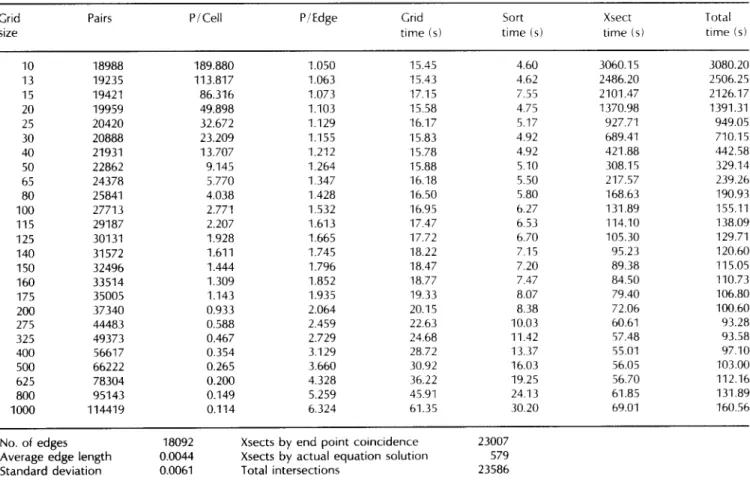
tried many values of G to learn the variation of computation time with G. For example, part of the Survey graph mentioned above was used to observe the variation of G. Average edge length was 0.0044 and there were 18092 edges. A total of 23586 intersections were found. For G = 10 the total time was 3080 s. This became 710 s when G was increased to 30. With G = 100 the time was 155 s. At G = 275 the timing figure was minimized: 93 s! After that, increasing G slightly increased the time, too. With G = 800 the time was 132 s and with G = 1000 the time became 161 s. It is noted that the optimal time for this case is within 5 0 % of the times obtained with grids from 115 x 115 up to 800 x 800. This demonstrates the extreme insensitivity of the time to grid size.
A very big example to date has been the handling of the Survey graph mentioned above. A total of 115973 edges of average length 0.0022 were submitted to the serial algorithm. A total of 135050 intersections were found in 683 s with a 650 x 650 grid. It is worth noting that while it may appear that 650 x 650 = 422500 cells is very inefficient in terms of storage, it should be recalled that not one word of storage is used for e m p t y cells.
Another very recent large example is a complete chip designed by Jim Guilford, a student of Professor Ed Rogers, at RPl's Computer Science Department. This chip has 1819064 edges, each of which is either horizontal or vertical. For the following timing figures, an optimized (for the rectilinear case) version of the program was used. General edges would slow it by a factor of t w o to three. The program used the standard
Table 2. Sample statistics for edge intersections for map 'Chikamagua area 3 - hydrography, roads, and trails.'
Grid Pairs P/Cell P/Edge Grid Sort Xsect Total
size time (s) time (s) time (s) time (s)
10 18988 189.880 1.050 15.45 4.60 3060.15 3080.20 13 19235 113.817 1.063 15.43 4.62 2486.20 2506.25 15 19421 86.316 1.073 17.15 7.55 2101.47 2126.17 20 19959 49.898 1.103 15.58 4.75 1370.98 1391.31 25 20420 32.672 1.129 16.17 5.17 927.71 949.05 30 20888 23.209 1.155 15.83 4.92 689.41 710.15 40 21931 13.707 1.212 15.78 4.92 421.88 442.58 50 22862 9.145 1.264 15.88 5.10 308.15 329.14 65 24378 5.770 1.347 16.18 5.50 217.57 239.26 80 25841 4.038 1.428 16.50 5.80 168.63 190.93 100 27713 2.771 1.532 16.95 6.27 131.89 155.11 115 29187 2.207 1.613 17.47 6.53 114.10 138.09 125 30131 1.928 1.665 17.72 6.70 105.30 129.71 140 31572 1.611 1.745 18.22 7.15 95.23 120.60 150 32496 1.444 1.796 18.47 7.20 89.38 115.05 160 33514 1.309 1.852 t8.77 7.47 84.50 110.73 175 35005 1.143 1.935 19.33 8.07 79.40 106.80 200 37340 0.933 2.064 20.15 8.38 72.06 100.60 275 44483 0.588 2.459 22.63 10.03 60.61 93.28 325 49373 0.467 2.729 24.68 11.42 57.48 93.58 400 56617 0.354 3.129 28.72 13.37 55.01 97.10 500 66222 0.265 3.660 30.92 16.03 56.05 103.00 625 78304 0.200 4.328 36.22 19.25 56.70 112.16 800 95143 0.149 5.259 45.91 24.13 61.85 131.89 1000 114419 0.114 6.324 61.35 30.20 69.01 160.56
No. of edges 18092 Xsects by end point coincidence 23007 Average edge length 0.0044 Xsects by actual equation solution 579 Standard deviation 0.0061 Total intersections 23586
Sun C compiler; commercial compilers may produce better code. On a Sun 4/280 with 32 Mbyte of real memory and using a 1200 x 1200 grid, 4577916 (cell, edge) pairs were calculated in 70 s whereas calculating the 6941110 intersections took 108 s (total time 178 s). The data structure was two simple square arrays of linked list headers. Each cell has a separate list for its horizontal and vertical edges. A 1500 x 1500 grid was a little bit slower: 5263144 (cell, edge) pairs, which were found in 79 s, and 111 s were spent to compute the intersections (total time 190
s).
Table 2 shows sample statistics for intersecting edges in a map titled 'Chikamagua area 3 - hydrography, roads, and trails' (uniprocessor). Table 3 is a summary of results from processing various data sets, separated with horizontal line~ in the table (again serial computation). Table 3 shows the effect of parallel computation. Figures 1 (a) and 1 (b), on the other hand, show the time and speed-up graphs for the Chikamagua map.
With these timing figures (timing starts when the array of edges is available for processing and excludes I/O), the authors believe that they have shown that there is hardly any need for complicated methods such as quadtrees and sweep algorithms.
DISCUSSION A N D C O N C L U S I O N
It may still be suggested that the first extension that would prove useful is to use a hierarchical grid to accommodate regions of the plot where the edges are somewhat clustered. This would, as a matter of fact, save time only when there are orders of magnitude variation in edge density. As soon as the cells become hierarchical, parts of the uniform grid algorithm that determine where (i.e. in which cells) an edge falls would become more complicated, thus slower. In fact, the preceding point is a very important objection to the uniform grid. Some parts of a real scene are frequently much denser than other parts so that a regular grid would appear not to work. Is a hierarchical technique, such as a quadtree, necessary?
The answer is no. First, even a quadtree cannot efficiently deal with all data sets. If there are n parallel edges separated by distances of n -~ for c > 1, then it takes more than quadratic time to build a quadtree (and a uniform grid for that matter) that has cells fine enough to distinguish the edges. The sweeping line algorithm would work well in this case, but it was noted earlier that the sweep paradigm cannot handle the red blue intersections.
Table 3. Summary of results from processing all data sets (serial computation)
Database Edges Length Standard
deviation Xsects Grid size Time (s) Risch e g g - YZ projection 5897 0.0355 0.0124 39666 100 194.24 XZ projection 5897 0.0391 0.0132 37415 115 193.18 XY projection 5897 0.0352 0.0131 40177 80 183.83 USA map
Shifted by 2 % and overlaid on itself Shifted by 10% and overlaid on itself
915 0.0186 0.0245 1078 125 4.97
1830 0.0184 0.0243 2430 140 14.38
1830 0.0180 0.0237 2348 125 12.57
Chikamagua area 1 - hydrography, 13712 0.0044 0.0084 15039 275 68.50
roads & trails (HR&T)
Area 2 - HR&T 14145 0.0049 0.0080 16595 275 71.11 Area 3 HR&T 18092 0.0044 0.0061 23586 275 93.28 Area 4 - HR&T 16425 0.0048 0.0076 20335 200 88.58 Area 5 - HR&T 12869 0.0053 0.0103 14978 275 62.93 Area 6 - HR&T 13871 0.0050 0.0080 16072 275 69.40 Area 7 - HR&T 13579 0.0134 0.0518 16640 160 188.76 Area 8 - HR&T 11937 0.0048 0.0098 13283 275 58.86
All sections - railroads 1122 0.0159 0.0543 1316 150 8.10
pipe & transmission lines 850 0.0277 0.0523 1211 115 7.95
railroads, pipe & transmission lines 1972 0.0206 0.0533 2745 115 22.28
Railroads, pipe & transmission 3944 0.0206 0.0533 13268 115 84.15
lines overlaid on itself
Hydrography, railroads, pipe & 55973 0.0023 0.0162 53426 500 323.09
transmission lines
Roads & trails, railroads, pipe 62045 0.0026 0.0106 81373 500 436.35
& transmission lines
Hydrography, roads & trails, 115973 0.0022 0.0115 135050 650 682.51
railroads, pipe & transmission lines
VLSI data XFACEA.MAG 436
VLSI data - XFACELL.MAG 1960
VLSI data - XFACELL.MAG 1960
(Rotated by 30 ° )
VLSI data - XFACELL.MAG 1960
(Rotated by 90 ° ) 0.0314 0.0467 0.0352 0.0467 0.0908 0.0852 0.0643 0.0852 1403 6488 6488 6488 150 65 125 65 5.22 16.87 32.48 18.67
On a more conceptual basis, there is evidence for assuming that data sets with one region that is exponentially more crowded than another are rare. In practice, scenes are resolution limited. People do not create scenes with enormous variations: if there is a large blank expanse, some detail will be added there; if there is a dense region, simplifying notation and approximations will be used. To quote Franklin et al. ~, 'We could also define such data sets out of existence as numerical analysts do with partial differential equations. Just as they consider only equations that satisfy a Lipschitz condition where the greatest slope of a curve is bounded, we might restrict ourselves to sequences of data sets where the densest region's density, relative to average density, remains bounded as n ~ oo.' 300 ~' 250 "O 8 200 150 E -- 1 0 0 - 0 5 0 - oi a \ - \ \ -
k
~" ~"e"e-~-_~.÷_e._~..e. ~..o.. e
l I I I I 3 6 9 12 15 Number of processors O. D "Ob
1 5 - 1 0 - 5 - - X ~ x x x x O" I I I I I 0 3 6 9 12 15 Number of processorsFigure 1. Time and speed-up graphs for Chikamagua map
Another extension is to handle curved edges, l his can be done without changing the general structure of uniform grid'
• The edges are no longer defined by endpoints but by the coordinates of splines, for instan(e.
• It is considerably more difficult to determine which cells a given curve occupies. If the curve is smooth, it can be enclosed in a box. (Again, it does not matter if a few extra cells are also included in this way.)If the curve is complicated, we can subdivide it until it is smooth and then use the bounding box.
• It is essential to find out whether two curves in the same cell intersect, and if that is the case, the parameter value. Efficient curve intersection is an area of active research. Obviously, the curves can be split into line segments, and intersected to obtain approximate crossing points, and then the result can be refined with a few iterations of Newton's rule. It is also known how curves can be approximated by quadratic parametrics for which closed form solutions are known.
• It is essential to sort (in, for example, HALO) the intersection points along each curve. If the curve is parametric this means that the point is needed as a parameter value, not just as (x, y). On the other hand, if the curve is in some other form but single- valued in say, x, then one can sort the points in x. A worthwhile addition to the uniform grid would be to compute, before preprocessing, a global 'slant' value for the whole data set showing the bias (if any) in the slopes of the edges. If the edges are slanted in some direction, then the grid can be placed parallel to that direction so that the number of grid cells spanned by the edges decreases.
Although the large scale and diverse data sets prove, in a strong sense, the efficiency and superiority of the uniform grid, analytical results, which assume some distribution and then prove asymptotic bounds, are certainly welcome. The authors regard the work in stochastic geometry (or geometric probability) quite relevant to this purpose. Although the expected performance of uniform grid is hard to analyse for all cases, Devroye's interesting monographS7 may provide the required theoretical basis. This remains to be seen. This paper was written to demonstrate, both by theoretical analysis and by implementation, that the uniform grid technique from computational geometry
Table 4. Summary of results from processing all data sets (parallel computation)
Database Edges Xsects Grid Time taken (s)
size
1 Processor 5 Processors 10 Processors 15 Processors
Risch egg - YZ projection 5897 39666 100 98.91 24.02 14.19 11.96
XZ projection 5897 37415 115 97.88 23.55 14.83 11.81
XY projection 5897 40177 80 92.33 20.33 12.36 10.40
Roads & trails, railroads, pipe 62045 81373 250 273.11 62.98 39.42 27.77
& transmission lines
leads to more efficient means of solving certain common operations in practice. In a nutshell, there are potential advantages in aiming research in computer graphics not only at producing fine representations ('pretty pictures') but also at identifying and solving the underlying algorithmic problems.
A C K N O W L E D G E M E N T S
The authors are grateful to Jeremy Weightman for his encouragement and kind invitation to write this paper. The first author thanks Ozay Oral and Mehmet Baray for their moral support. The second author's research is supported by the National Science Foundation under PYI grant no. DMC-8351942.
Mention of commercial products in this paper does not necessarily imply endorsement.
R E F E R E N C E S
1 Guibas, L J and Stolfi, J 'Ruler, compass, and
computer: the design and analysis of geometric algorithms' in Earnshaw, R A (ed)
Theoretical
foundations of computer graphics and CAD
NATO ASI Series Vol F40 Springer-Verlag (1988) pp 111-165 2 Franklin, W R 'Combinatorics of hidden surface algorithms'PhD thesis
(alsoTechnical Report TR-
12-78)
Center for Research in Computing Technology, Harvard University Cambridge MA, USA (1978) 3 Edelsbrunner, HAlgorithms in combinatorial
geometry
Springer-Verlag (1987)4 Preparata, F P and Shamos, M I
Computational
geometry: an introduction
Texts and Monographs in Computer Science, Springer-Verlag (1985) 5 Greene, D H and Knuth, D EMathematics for the
analysis of algorithms
Progress in Computer Science Vol 1 Birkh~user, Boston, MA, USA (1981)6 Bentley, J L and Ottmann, T A 'Algorithms for
reporting and counting geometric intersections'
IEEE Trans. Comput.
Vol C-28 No 9 (1979) pp 643-6477 Chazelle, B 'Reporting and counting arbitrary planar intersections'
Technical Report CS-83-16
Department of Computer Science, Brown University, Providence, RI, USA (1983)
8 Chazelle, B and Edelsbrunner, H 'An optimal
algorithm for intersecting line segments in the plane'
Proc. 29th Ann. Conf. Foundations of
Computer Science
White Plains, New York, NY, USA (October 1988)9 Mairson, H G and Stolfi, J 'Reporting and counting
intersections between two sets of line segments' in
Earnshaw, R A (ed)
Theoretical foundations
ofcomputer graphics and CAD
NATO ASI Series Vol F40 Springer-Verlag (1988) pp 307-32510 Hart, S and Sharir, M 'Nonlinearity of Davenport-
Schinzel sequences and of generalized path compression schemes'
Combinatorica
Vol 6 No 2 (1986) pp 151-17711 Myers, E W 'An O(E log E+I) expected time
algorithm for the planar segment intersection problem'
SIAM J. Comput.
Vol 14 No 3 (1983) pp 625-63712 Franklin, W R, Wu, P Y I:, Samaddar, S and Nichols,
M 'Prolog and geometry projects'
IEEE Comput.
Graph. Appl.
Vol 6 No 11 (1986) pp 46-5513 Franklin, W R 'Cartographics errors symptomatic
of underlying algebra problems'
Proc. Int. Syrup.
Spatial Data Handling
Vol 1, Zurich, Switzerland (1984) pp 190-20814 Forrest, A R 'Computational geometry in practice'
in Earnshaw, R A (ed)
Fundamental algorithms for
computer graphics
NATO ASI Series Vol F17 Springer-Verlag (1985) pp 707-72415 Akman, V 'Geometry and graphics applied to robotics' in Earnshaw, R A (ed)
Theoretical
foundations of computer graphics and CAD
NATO ASI Series Vol F40 Springer-Verlag (1988) pp 619-63816 Forrest, A R 'Geometric computing environments:
some tentative thoughts' in Earnshaw, R A (ed)
Theoretical foundations of computer graphics and
CAD
NATO ASI Series Vol F40 Springer-Verlag (1988) pp 185-19717 Akman, V
Unobstructed shortest paths in polyhedral
environments
Lecture Notes in Computer Science Vol 251 Springer-Verlag (1987)18 Asano, T, Edahiro, M, Imai, H, Iri, M and Murota, K
'Practical use of bucketing techniques in compu- tational geometry' in Toussaint, G T (ed)
Computational geometry
Elsevier Science Publishers (North Holland)(1985) pp 153-19519 Sutherland, I E, Sproull, R I: and Schumacker, R A
'A characterization of ten hidden surface algorithms'
ACM Comput. Surv.
Vol 6 No 1 (1974) pp 1-5520 Bentley, J L 'Multidimensional binary search trees
used for associative searching'
Commun. ACM
Vol 18 No 9 (1975) pp 509-51721 Finkel, R A and Bentley, J L 'Quad trees: a data
structure for retrieval on composite keys'
Acta
Informatica
Vol 4 (1974) pp 1-922 Meagher, D J 'Geometric modeling using octree
encoding'
Comput. Graph. Image Process.
Vol 19 No 2 (1982) pp 129-14723 Appel, A, Rohlf, F J and Stein, A J 'The haloed line
effect for hidden line elimination'
ACM Comput.
Graph. (Proc. SIGGRAPH'79)
Vol 13 No 2 (1979) pp 151-15624
25
Arnold, D and de Ruiter, B 'Editorial'
Comput.
Graph. Forum
Vol 6 No 2 (May 1987) pp 75-76Franklin, W R and Akman, V 'A simple and efficient
haloed line algorithm for hidden line elimination'
Comput. Graph. Forum
Vol 6 No 2 (1987) pp 103-10926 Kernighan, B W and Plauger, P H Soitware Tools Addison-Wesley Inc, USA (1976)
27 Franklin, W R 'Efficient polyhedron intersection and union' Proc. Graphics Interface '82 Toronto, Canada (1982) pp 73 80
28 Franklin, W R and Akman, V 'Reconstructing visible
regions from visible segments' BIT Vol 26 (1986) pp 430- 441
29 Franklin, W R 'A simplified map overlay algorithm'
Proc. Harvard Comput. Graph. Conf. Cambridge, MA, USA (1983)
30 Franklin, W R 'Adaptive grids for geometric operations' Proc. 6th Int. Syrup. on Automated
Cartography (Auto-Carto Six) Vol 2 Ottawa, Canada (1983) pp 230 239
31 Franklin, W R and Akman, V 'Adaptive grid for
polyhedral visibility in object space: an implementa- tion' Comput. J. Vol 31 No 1 (1988) pp 56 60 32 McKenna, M 'Worst case optimal hidden surface
removal' ACIV/ Trans. Graph. Vol 6 No 1 (1987) pp 19-28
33 Franklin, W R 'A linear time exact hidden surface algorithm' ACM Comput. Graph. (Pro(. 51GGRAPH "80) Vol 14 No 3 (1980) pp 117 -123
34 Franklin, W R, Chandrasekhar, N, Kankanhalli, M, Seshan, M and Akman, V 'Efficiency of uniform grids
for intersection detection on serial and parallel machines' in Magnenat-Thalmann, N and Thai-
mann, D (eds) New trends in computer graphics
( Proc. Computer Graphics International'88) Springer- Verlag (1988)
35 Chandrasekhar, N and Seshan, M 'The efficiency of uniform grid for computing intersections' MS
thesis Electrical, Computer, and Systems Engineering Dept, Rensselaer Polytechnic Institute, Troy, NY, USA (1987)
36 Kankanhalli, M 'Uniform grids for line intersection
in parallel' MS thesis Electrical, Computer, and Systems Engineering Dept, Rensselaer Polytechnic Institute, Troy, NY, USA (1988)
37 Devroye, L Lecture notes on bucket algorithms Progress in Computer Science Vol 6, Birkh~user, Boston, MA, USA (1986)