Brought to you by | Kadir Has University Authenticated Download Date | 12/12/19 12:07 PM

Frequenz 58(2004) 7-8

178

EM Based Stochastic Maximum

Likelihood Approach for Localization

of Near-field Sources in 3-D

Abstract

The goal of this paper is to estimate the locations of unknown sources in 3-D space from the data collected by a 2-D rectangular array. Various studies employing different estimation methods under near-field and far-field assumptions were presented in the past. In most of the previous studies, location estimations of sources at the same plane with the antenna array were carried out by using algorithms having constraints for various situa-tions indeed. In this study, location estimasitua-tions of sources that are placed at a different plane from the antenna array is given. In other words, locations of sources in 3-D space is estimated by using a 2-D rectangular array. Maximum likelihood (ML) method is chosen as the estimator since it has a better resolution performance than the conventional methods in the presence of less number and highly correlated source signal samples and low signal to noise ratio. Besides these superiorities, stability, asymptotic unbiasedness, asymptotic minimum vari-ance properties as well as no restrictions on the antenna array are motivated the application of ML approach. Despite these advantages, ML estimator has computational complexity. However, this problem is tackled by the application of Expectation/Maximization (EM) iterative algorithm which converts the multidimensional search problem to one dimensional parallel search problems in order to prevent computational complexity. EM itera-tive algorithm is therefore adapted to the localization problem by the data (complete data) assumed to arrive to the sensors separately instead of observed data (incomplete data). Furthermore, performance of the proposed algorithm is tested by deriving Cramer-Rao bounds based on the concentrated likelihood approach. Finally, the applicability and effectiveness of the proposed algorithm is illustrated by some numerical simulations

Index Terms

Maximum Likelihood estimation, Expectation, Maximization algorithm, Antenna arrays, Localization of near-field sources in 3-D space

1. Introduction

In the last decades, the basic interest in the array processing re-search turned towards the developing algorithms for localization of sources by using passive sensor array. These algorithms were applied to radar, sonar, radio astronomy, geophysics, seismolo-gy, robotic and biomedicine [1-4]. In the last, many studies were presented for solution to the problem of direction of arrival esti-mations of narrow-band far-field sources [5-21]. In far-field sce-narios, each source location could be characterized by only the azimuth and/or elevation since waves impinging to antenna ar-ray were considered as plane waves. When the sources are locat-ed close to the array (i.e., near-field), the inherent curvature of the waveforms can no longer be neglected. Therefore, the spheri-cal wavefronts in the near-field scenario must be considered and the location of each source has to be parametrized in terms of the direction of arrival (azimuth and/or elevation; DOA) together with range [22-24]. However, in [22-24], it was assumed that all sources were at the same plane with antenna array which intro-duces some restrictions to some applications in the real world.

Localization of sources at the different plane with antenna ar-ray is more applicable to the real world arar-ray processing prob-lems. Primary research results presented under this assumption were for localization of narrow-band far-field source signals [25-27]. Moreover, recent research results on localization of near-field narrow-band sources in 3-D space were also presented [28, 29]. Faced with inability to completely evaluate performances of optimal 3-D near-field localization approaches from [28,29], it is reasonable to resort to a asymptotically optimal estimators.

The localization of the near-field sources in 3-D space is in gen-eral nontrivial, since localization of near-field sources requires estimation of the azimuth and elevation together with the range parameters. Recently, an algorithm using 3-D Music with polyno-mial rooting has been developed [28]. High-order subspace based algorithms were introduced in [29]. In contrast to suboptimal ap-proaches proposed in [28,29], we now investigate an alternative

1 Electronics and Communication Program, Technical Vocational School, Kadir Has University Bahcelievler, Turkey

2 Department of Electrical Engineering, Istanbul University Avcilar, Istanbul, Turkey

3 Electronics and Communication Engineering Department, Istanbul Technical University Maslak, Istanbul, Turkey

estimator that is asymptotically efficient. Due to many attrac-tive properties of maximum likelihood (ML) estimation meth-ods such as consistency, asymptotic unbiasednes and asymptotic minimum variance, we concentrate on ML method for localiza-tion of near-field sources in 3-D space. Furthermore it has a bet-ter resolution performance than the other methods in the pres-ence of less number and highly correlated source signal samples and low signal to noise ratios. Besides these superiorities, it also brings no restrictions on the antenna array structure. Regarding the assumption on the narrow-band source signals, there are two different types of models. These two models lead corresponding ML solutions. The models are

i. Deterministic Model (DM) which assumes the signals to be unknown but deterministic (i. e., the same in all realizations) ii. Stochastic Model (SM) which assumes the signals to be

ran-dom.

ML methods corresponding to the signal models (i) and (ii) are termed deterministic ML and stochastic ML respectively. Ex-pectation/Maximization (EM) based deterministic ML (signal model (i)) near-field location estimator have been studied in [30]. The goal of the present paper is to provide a stochastic ML ap-proach for the estimation of the DOA and range parameters of near-field sources. However, calculation of ML estimation from corresponding likelihood function for the stochastic case results in difficult nonlinear constrained optimization problem, which must be solved iteratively. We therefore employed the EM itera-tive method for obtaining ML estimator. The most important fea-ture of the algorithm is that it decomposes the observed data into its signal components and then estimates the parameters of each signal component separately.

The asymptotical performance of an stochastic ML 3-D near-field localization technique is analyzed via the derivation of Cra-mer Rao Bounds (CRB) which provides benchmarks for evaluat-ing the performance of actual estimators. The technique for the derivation of CRBs used here in relies as modulators of the log-likelihood function by replacing the nuisance parameters with their ML estimates. It therefore avoids the process of explicitly calculating and inverting the entire Fisher Information Matrix (FIM). We substitute the ML estimates of the array observation covariance matrix to obtain concentrated covariance matrix. We then calculated the CRBs for location parameters of near-field sources in 3-D space by modifying the bounds presented in [31].

Rg. 1: Near-field scenario with a 2-D linear array

The remainder of the paper is organized as follows. The sig-nal model for 3-D near-field scenario is presented in section 2. In section 3, the stochastic ML estimator and the corresponding as-sumptions on the signal model are outlined. Moreover, the itera-tive EM algorithm for obtaining ML estimates from correspond-ing stochastic cost function is introduced. While in section 4, the performance of the stochastic ML method is evaluated based on the concentrated ML approach to obtain CRBs. In section 5, sim-ulation results are presented. Finally, some conclusions of the work are reported.

2. Signal Model

Consider a near-field scenario in which narrowband signals from d sources received by an Κ χ L element antenna array. Let the ar-ray center be the phase reference point with index '(0,0)' as de-picted in Figure 1.

Assuming 2-D rectangular uniform linear array consisting of omnidirectional sensors with interelement spacing Δ along each axes, we write the output of the (k,l)& sensor with narrowband,

co-channel signal at time I, as,

(D

(=1

where s/(/„) denotes the complex envelope of the /* source signal, "«('») is an additive complex Gaussian sensor noise and τ*Χ/) is the phase difference of the i* signal collected at sensor (k,[) with respect to the ith signal collected at reference sensor '(0,0)'. Due

to our narrowband assumption, the phase difference is given by

(2)

where λ· c/2ji./o is the wavelength corresponding to the center frequency fa of the signals travelling at a velocity c. The distance between ι * source and the (λ,/)* sensor equals

(3)

The plane wave approximation of far-field sources is obtained by retaining only term up to the first power of Δ/Λ and its multi-plier in the binomial expansion of (3). Since the near field sourc-es are of intersourc-est in this paper, we should include an extra term to approximate the effect of spherical waves. By retaining terms up to the second power of Δ/r, and its multiplier in the binomial

ex-pansion of (3), such an approximation can therefore be obtained. We then arrive at the Fresnel approximation of the distance:

2ιί

',+^-(ΐ-™'βΧθ,) 2r

sin 0,sin2f>,j. (4)

If we substitute (4) in (2). we obtain the phase difference <V + */ + AW] as ('')=(— sin^cos^U-i— (ΐ-Λι^,οο·2^)]*1 (5) where 2πΔ . „ ,=——stnfl,cosfl),, 2χΔ . ·* λ >>=£*_^ί ,=^-*Se, **! ,^Ι-^Ο^φ,), **! (6)

Then, the noise corrupted array measurements at the sensor can be approximately expressed as:

1=1

(7)

For a collection of observed outputs of Κ χ L sensors in 2-D ar-ray x(/J - [x^C.) Xi^ft,)]7". the model (7) is written more compactly in matrix notation as

(8)

where the super vector x(/») consists of χ/(4,)

x*MI./tti)]r whicn is output of only one column sub-array of the 2-D rectangular array, s(/„) - [$/(/„) ... .v(f„)]r is the collection of d source signals impinging to 2-D array, n(f„) - [n/^^i/J ... n^nu(rjl)]r is super Gaussian complex vector with zero-mean and known spatial covariance σ2!, which consists of sub-array noise vectors one forming as n<(f„) - [nj^X/O ... nj^XOl^ Α(θ,φ,Γ) ·= [Α\(θ,φ,τ)...Α^,θ,φ,τ)] is the arrays steering matrix in the near-field scenario which is known as a function of unknown set of parameters 0 - [ft ... 0,]Γ, φ - [φι ... φλτ, r -[r, ... rrf]r, consisting of subarray steering vectors one forming as Λι(θ,φ,ή -1*^(^9^) - «inuiftV·1)^*1«1 «/(ftflW) is ^ sub-array steer-ing vector for /* source, in the »,,Ι(θ,φ,ι) - [e'^- ni*0, ..., 1,

We are interested in stochastic ML approach in this paper for the estimation of 3-D near-field source location parameters [θ,φ*] - [(ή,φ,Γι) ... (ξ,,φ,,Γ^)) from η observations je - [xr(l), ..., xr(N)]rmade from (8). The data for this problem consists of a set of discrete samples (x(Ar); l S * S N] of the process x(r„). Our approach is to derive an iterative stochastic ML estimator based

Frequenz 58(2004) 7-8

179

Frequenz 58(2004)

7-8

on the EM algorithm, that performs joint sample covariance and location parameters estimation in alternating steps.

3. Stochastic ML Estimator

In this section we derive the stochastic ML estimator for the prob-lem defined above. To describe stochastic ML estimator's deri-vation, we made the following assumptions on the signal model

(7):

AS1: The source signal &(k) is temporally and spatially

uncorre-lated circular complex Gaussian random process with zero-mean and nonsingular unknown covariance matrix K,,

for all Λ, an (9)

where &,,*, is the Kronecker delta (&,,*2 ·= 1 if fci = Jtj and 0

oth-erwise), (·) is the conjugate transpose and (·)Γ is the transpose

of a matrix.

AS2: The additive noise vector n(Jfc) is temporally and spatially uncorrelated circular complex Gaussian process with zero-mean and standard! derivative o2 as

where Kx is the sample covariance matrix. Then the negative

log-likelihood function becomes

(17)

Then, the ML estimates of [θ,φ,τ] and s are those which local-ly minimize the negative log-likelihood function (IS). However, minimizing (IS) is a nonlinear multiparameter optimization problem and does not yield to a closed-form solution. Solutions of such problems usually requires numerical methods, such as the methods of Scoring, Newton-Raphson or some other gradient search algorithm. However, for the problem at hand, these numer-ical methods tend to be computationally complex. Thus, a com-putationally efficient iterative algorithm is required for solving resulting optimization problem. To solve this problem, we pro-pose a stochastic ML estimation technique based on the EM al-gorithm which decomposes the observed data into its signal com-ponents and then estimates the parameters of each signal compo-nents separately. Thus, multidimensional maximization has been reduced to separate one dimensional maximizations yielding an easier problem in general. Moreover, the EM algorithm iterates as the parameter updates in a manner which guarantees an in-crease in the likelihood function.

forall *, an

(10)

D

AS3: The source signal s(kj) and the noise η(Λ2) are

uncorre-lated for all *, and fc2.

Based on the assumptions AS2 and AS3, the array observa-tions χ are Gaussian distributed with zero-mean and covariance Κχ(θ,φ,ι·,Κ,),ϊ.β.,

(12)

=A(0,9.r)K,Ali(e,?,r)+<T2L

Then joint probability density function of the observation χ = \(k), k = 1, ...,N] given [θ,φ,Γ,Κ,] can be written as follows:

expl —ι

The joint probability function (13) can also be written as

(14)

where tr is the trace. The negative log-likelihood function (after neglecting unnecessary terms) is

mdetK,--iJ K^xUVU) ί

N I *=i J

(15)

AS2 implies that, by the law of large numbers x(A) is second-order ergodic, i. e.,

3.1 EM Algorithm

The formulation of the estimation problem at hand in terms of the actual data sample (incomplete-data) and a hypothetical data set (complete-data) allows us to apply the EM algorithm. To be able to easily apply the EM algorithm the complete data must be chosen in such a way that:

- the complete data log-likelihood function is easily maximized

and

- the complete data log-likelihood function can be easily estimat-ed from the incomplete data. The choice for the complete data vector is obtained from hypothetical independent observations of each incident wave as

\<i<d

where n,()fc) is the Gaussian noise vector belongs to /* signal. The complete-data vector y/(/t) is the set of Ν samples of d inde-pendent Gaussian vectors with the /* vector y,(k) having mean Ai(0,q>,T)s,(k) and with identical covariance (fl/d. Thus, the com-plete-data y,(Jfc) and the incomplete data x(Jfc) is can be related by Under AS1, the covariance matrix K, is a diagonal matrix K, = diag[ct/, .... aj[, then the complete data y/(/„) is the Gaussian process with mean zero and covariance

(19)

Then the log-likelihood function of the complete datay/Ot) is

I

K;

Ey,(*)y*(*)L

'*=! J

(20)

At the (ρ + ΐ)Λ iteration, two step EM algorithm for our

prob-lem has the following steps:

Expectation Step: Compute conditional expectation of the suf-ficient statistics for the complete data log-likelihood. The suffi-cient statistics is the sample covariance of the complete-data,

180

X

(21) *=ι

At the 0» + 1)Λ iteration, expected value of K/f1 given K£ and

K?,is

(2

In (22), K?( and Kf can be obtained from the estimates of

near-field parameters [θ',φ",^} at iteration p, J = \(θ',φ',Γ')κζ\Η(θ',φ'.Γ')+σ21

(23)

Maximization Step: The conditional expectation of the

suf-ficient statistics obtained in Expectation Step is substituted in (20). Then the complete-data likelihood function is maximized with respect to the parameters to be estimated {ή,φ,Γ/,Κ,]:

(24)

The determinant of KJ( can be obtained by using the spectral

decomposition. One eigenvector of Ky/ is Ai(e,<p,i)l\A,(e,<p,r)\,

ATx L - I other mutually orthogonal eigenvector can be chosen from orthogonal complement of Λ^θ,φ,τ) and are equal to cfld. Then the eigenvalue corresponding to the distinct eigenvector is

(25)

Since the inverse of K;/ is required in (24), it could be

deter-mined by employing matrix inverse lemma as

-Obtain*^1 from (22),

- Substitute K/*1 in (27), and then solve (27) for {6Γ1, <fT\ ΓΓ1].

- Substitute the estimates [ΘΓ\ φΓι, τΓι] in (28), then

com-pute oTl,

3. Continue this process until [Q,(#,r(J and a, converges.

For a sufficiently good initialization, this algorithm converges rapidly to the ML estimate of the near-field parameters [θ,φ,?] and the source signals K,.

4. Cramer Rao Bounds

The CRB provides a lower bound on the error variance of any unbiased estimators. In particular, it provides an asymptotic near-field source location estimator. The parameter of interest is τ = [θΓφΙίτΓ]Γ. To focus on the parameters of interest, we shall use

a concentrated likelihood approach to obtain the CRB [31]. Then the ij/h element of the Fisher Information Matrix is given by

(29)

Then the determinant of KJ( can be written as

where [·]» is defined as the almost sure (a.s.) limit of [·], and K, is the concentrated covariance after substituting the ML esti-mates Kx for Kx.

The ML estimate of K, can be obtained as

κ.=[A^A!' Α*Κ

Α[Α"ΑΤ' -σ

[A^A]"'

where we have suppressed the dependence of A on (θ,φ,Γ). It is well known that K, -» K, almost surely under mild conditions. Concentrating the covariance K, with respect to K, yields

d_ σ2 (26) K, = AK.A" +σ2/ = PKxP+o2F where Ρ ^ A[ A^A]"' A* and F ^ I - P. (31) (32)

If we substitute the eigenvalues and the inverse of KT/ into (24),

and maximizing (24) for 04 > 0, the estimates of near-field param-eters become

We are now ready to evaluate CRB. Taking the first derivative <5Κ,/Λί, the following can be obtained

s- =Ρ,ΚχΡ+ΡΚχΡ,+σ2Ρ/. ₍₃₃₎

Μ ,φ4

(27)

whereP/=<?P/<?ii.

We will make use of the properties of projection matrix to ob-tain,

PT =0

- (28)

Based on this results, the steps of the proposed unconditional ML algorithm are summarized as follows:

Repeat steps 1-3 for / - 1 d 1. Given {ftV.r,0 a?}, p - 0,

(34) (35) (36)

Thus, taking the limit JV-» <» of (33)

(37)

Frequenz 58(2004)

7-8

Using (29) and the last result, we have

181

Frequenz 58(2004)

7-8

182

Ι

(τ)=ΛΓΐτ[κ-

(ρ

Κ

Ρ+ΡΚ

Ρ

+σ

Ρ/)

Next, we note that

where (·)* is the pseudo inverse of

(-)-To evaluate (38) explicitly, we consider its nine terms:

[2.]

tr[K-'PK

P

K-'P,K

,p]=tr[pP

K;'P,K

]

tr[K;'PK

P

K-'PK,P,]=tr[PP

PP,]

0

Plugging these results in (38), we have

Here, (38) (39) =-ί-Α»

ΑΚ.Α*-ΑΚ.[-σ

^

\t

-^-Α^ΑΚ,+Ι A*

σ /

Using (SO) in (49), produces

(51) (41)

(42)

Finally, using (51), we have CRB upon inversion

(52)

where Θ denotes the element-wise matrix products

(43) (44)

=-ft[AfF

A

(A*A)"

] (45)

(46)

5. Simulations

To illustrate the the effectiveness and applicability of the pro-posed method, we consider the following scenarios.

Case 1: A Uniform rectangular linear array of AT- L - 3 totally 9 sensors with inter-element spacing Δ = λ/2 was used to estimate the locations of two sources located at [θ,,φ,,τ,] = [24°, 80°, 2λ] and [&i,(pi,ti] = [34°, 5°, 1.6Λ]. The number of the snapshots (N) set to 80 and the SNR was varied from 0 to 30 dB. The proposed method was tested for Λ/= 100 independent trials. The resulting RMSE of the estimated DOAs (azimuths and elevations in de-grees) and ranges in wavelength are shown in Fig. 2, Fig. 3 and Fig. 4. The results were compared with the Cramer-Rao Bounds.

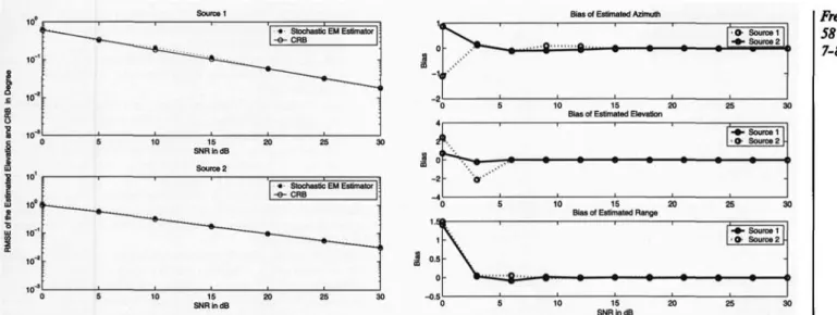
Case 2: To illustrate bias and convergence rate of the

estima-tor, we consider a new scenerio. A Uniform rectangular linear array of AT- L - 5 totally 25 sensors with inter-element spacing Δ = λ/2 was used to estimate the locations of two sources locat-ed at [6Mft,r,J = [70°, 24°, 4.5AJ and {fc,<fc,r2] = [70°, -24°, 7AJ.

(47)

(48)

SNRhdB Rg. 2: RMSE of the estimated azimuths

Source 1 Bias of Estimated Azimuth

Fig. 3: RMSE of the estimated elevations

10 15 20 Bias of Estimated Elevation

10 15 20 Bias of Estimated Range

10 15 20 SNR in dB

Ο· Source 1

·»- Source 2

Rg. 5: Bias of the estimated azimuths.elevations and ranges versus SNR

Frequenz 58(2004)

7-8

Source! _{Bias of Estimated Azimuth}

SNR in dB Rg. 4: RMSE of the estimated ranges

The number of the snapshots (N) set to 1000 and the SNR was varied from 0 to 30 dB and The proposed method was tested for M= 500 independent trials. Bias of the estimated azimuth, eleva-tion and range versus SNR and iteraeleva-tions number are shown in Fig. 5 and Fig. 6 respectively. Also, the convergence rates of the estimated source parameters are shown in Fig. 7.

Based on the simulation results we made the following obser-vations:

- For a sufficiently good initialization, proposed algorithm con-verges rapidly to the ML estimate of [θ,φ,Γ J and K,. Since the spatial structure of the array matrix is known, then the good initial estimates of the steering matrix can be obtained from MUSIC and ESPRIT algorithms.

- For high SNRs the RMSEs obtained from simulations becomes almost identical to the CRB results derived by modifying the results in [31].

- As expected, for a high enough SNR, the estimator is essential-ly unbiased. Moreover, for larger iterations, it is verified that the mean equals to true value.

- In the near-field scenario, it is observed that the proposed al-gorithm converges in around 10 to 20 steps.

40 60 80 Bias of Estimated Elevation

-10 ( ^S. ·+· Source 1 >f_ ·Ο· SourceZ p ί ) 20 40 60 80 100 1S Bias of Estimated Azimuth

40 60 Iteration Number

Rg. 6: Bias of the estimated azimuths.elevations and ranges versus iteration number

Convergence Rate of Estimated Azimuth 1

\

Λ

\

\

\

Λ

I -·- Source?] | · O· Source 2 |

20 40 60 80 100 12 Convergence Rate of Estimated Range

I -·- Source?] | ' O' Source 2

\

Rg. 7: Convergence of the proposed algorithm of estimated azimuths.elevations and ranges

6. Conclusions

In this paper, we have described a stochastic approach to esti-mate the parameters of near-field sources in 3-D space. We de-rived an EM based iterative method for obtaining ML estimator.

Furthermore the performance of the proposed method is stud-ied based on the derivation of Cramer-Rao bounds from concen-trated likelihood function. We also presented Monte Carlo sim-ulations to verify the theoretically predicted estimator's perfor-mance. The examples demonstrated that the proposed stochastic

ML achieve the concentrated CRB for moderate and high SNR

183

Frequenz values. Furthermore, they also demonstrated that proposed sto-58 (2004) chastic ML has nearly zero bias, and it converges rapidly for all

7-8 source location parameters.

This work was supported by The Research Fund of The University of Istanbul. Project Numb: 220/29042004.

References

[1] Wong, K. T; Zoltowski, M. D.: Orthogonal Velocity-hydrophone ES-PRIT for Sonar Source Localization. Proceedings of the Conference OCEANS '96. MTS/IEEE. Prospects for the 21st Century 6 (1996). [2] Asono, F.; Asoh, H.: Matsui, T.: Sound source localization and signal

seperation for Office robot Jijo-2. Proceedings of the IEEE Internation-al Conference on Multisensor Fusion and Integration for Intelligent Systems, 1999.

[3] Arslan, G.; Sakarya. F. A.: A unified neural-network-based speaker lo-calization technique. IEEE Transactions on Neural Networks, July, vol.

11, issue 4,2000.

[4] Owsley, N. L.: Array phonocardiography. The IEEE Symposium on Adaptive Systems for Signal Processing, Communications, and Con-trol, AS-SPCC, 2000.

[S] Feder, M.; Weinstein, E.: Parameter Estimation of Superimposed Sig-nals Using the EM Algorithm. IEEE Transaction on Acoustic, Speech, and Signal Processing 36 (April 1988) 477-489.

[6] Roy, R.; Kailath, T.: ESPRIT-Estimation of Signal Parameters via Rota-tional Invariance Techniques. IEEE Transaction on Acoustic, Speech, and Signal Processing 37 (July 1989) 7,984-995.

[7] Stoica, P.; Nehorai, A.: Music, maximum likelihood, and Cramer-Rao bound. IEEE Transaction on Acoustics. Speech, and Signal Processing. 37 (May 1989) 5.720-741.

[8] Stoica, P.; Nehorai, A.: Music, maximum likelihood, and Cramer-Rao bound: Further results and comparisions. IEEE Transaction on Acous-tics, Speech, and Signal Processing 38 (May 1989) 12,2140-2150. [9] Miller, M. I.; Fuhrmann, D. R.: Maximum-Likelihood Narrow-Band

Di-rection Finding and the EM Algorithm. IEEE Transaction on Acous-tics, Speech, and Signal Processing 38 (September 1990) 9.1560-1577. [10] Stoica, P.. Nehorai, A.: Performance Comparison of Subspace

Rota-tion and MUSIC Methods for DirecRota-tion EstimaRota-tion. IEEE Fifth ASSP Workshop on Spectrum Estimation and Modelling, 1990,357-361. [11] Ottersten, B., Viberg, M., Kailath, T.: Analysis of Subspace Fitting and

ML Techniques for Parameter Estimation from Sensor Array Data. IEEE Transaction on Signal Processing, 40 (March 1992) 590-600. [12] Weiss, A. J.; Friedlander B.: Pre-Processing for Direction Finding with

Minimal Variance Degradation. IEEE Transaction on Signal Process-ing 42 (June 1994) 6.1478-1485.

[13] Friedlander, B., Francos J. M.: Estimation of Amplitude and Phase pa-rameters of Multicomponent Signals. IEEE Transaction on Signal Pro-cessing 43 (1995) 4,917-926.

[14] Zeira, A. Friedlander, B.: Array Processing Using Parametric Signal Models. IEEE International Conference on Acoustic, Speech, and Sig-nal Processing (ICASSP-95), 1995.1667-1680.

[15] Abatzoglou, T. J., Steakley, B. C.: Comparision of Maximum Likeli-hood Estimators of Mean Wind Velocity from Radar/Lidar Returns. IEEE 13th Asilomar Conference on Signals, Systems and Computers,

1996.156-160.

[16] Krim, H.; Viberg, M.: Two decades of array processing research: The parametric approach. IEEE Signal Processing Magazine 13 (July 1996) 4,67-94.

[17] Sheinvald, J.; Wax, M.; Weiss. A. J.: On Maximum Likelihood Location of Coherent Signals. IEEE Transaction on Signal Processing 44 (Oct.

1996)10,2475-2482.

[18] Gershmen, A. B.; Bonnie J. F.: A Note on Most Favorable Array Geom-etries for DOA Estimation and Array Interpolation. IEEE Signal Pro-cessing Letters 4 (1997) 8.232-235.

[19] Haardt, M.: Efficient One-, Two. and Multidimensional High-Resolu-tion Array Signal Processing. Ph.D. dissertaHigh-Resolu-tion. Technische Univer-sität München, 1997.

[20] Kailath, T; Poor. H. V: Detection of Stochastic Processes. IEEE Trans-action on Information Theory. 44 (Oct. 1998) 6.2230-2259. [21] Perry, R.; Buckley. K.: Maximum Likelihood Source Localization

Us-ing the EM Algorithm to Incorporate Prior Distribution. First IEEE Sensor Array and Multichannel Signal Processing Workshop (16-17 March 2000) 351-355.

[22] Challa,R.N.; Shamsunder, S.: High-Order Subspace-Based Algorithms for Passive Localization of Near-Field Sources, in: Proc. 29th Asimolar Conf. on Signals, Systems, and Computers 2 (Nov. 1995) Pacific Grove, CA., 777-781.

[23] Abed-Meraim, K.; Hua, Y.; Belouchrani, A.: Second-Order Near-Field Souce Localization: Algorithm and Performance Analysis, in: Proc. 30th Asimolar Conf. on Signals, Systems and Computers (Oct. 1996). [24] Kabaoglu, N.; Cirpan, H.; Cekli, E.; Paker, S.: Deterministic Maximum

Likelihood Approach for 3-D Near-Field Source Localization. AEU, International Journal of Electronics and Communication, 57 (2003) 5345-350.

[25] Yuen, N.; Friedlander, B.: Performance Analysis of Higher Order ES-PRIT for Localization of Near-Field Souces. IEEE Trans, on Signal Pro-cessing 46 (March 1998) 709-719.

[26] Van der Veen, A. J.: Ober, P. B.; Deprettere, E. D.: Azimuth and Eleva-tion ComputaEleva-tion in High ResoluEleva-tion DOA EstimaEleva-tion. IEEE Transac-tion on Signal Processing 40 (July 1992) 1828-1832.

[27] Swindlehurst, A. L.; Kailath, T: Azimuth/Elevation Direction Finding Using Regular Array Geometries. IEEE Transaction on Aerospace and Electronic Systems 29 (Jan. 1993) 145-156.

[28] Zoltowski, M. D.; Haardt, M.; Mathews C. P.: Closed-form 2-D Angle Estimation with Rectangular Arrays in Element Space or Beamspace via Unitary ESPRIT. IEEE Transaction on Signal Processing 44 (Feb. 1996)316-328.

[29] Hung, H.; Change, S.; Wu C.: 3-D Music with Polynomial Rooting for Near-Field Source Localization. International Conference on Acous-tic, Speech, and Signal Processing (1CASSP-96) 6 (May 1996) Atlanta, Georgia, 3065-3069.

[30] Challa, R. N.; Shamsunder, S.: Passive Near-Field Localization of Mul-tiple Non-Gaussian Sources in 3-D using Cumulants. Signal Processing 65(1998)39-53.

[31] Hochwald. B.; Nehorai. A.: Concentrated Cramer Rao Bound Expres-sion. IEEE Trans, on Information Theory 40 (March 1994) 363-371.

Nihat Kabaoglu

Electronics and Communication Program Technical Vocational School

Kadir Has University Bahcelievler 34188. Turkey Hakan A. Cirpan

Department of Electrical Engineering Istanbul University Avcilar

34850 Istanbul Turkey

e-mail: hcirpan@istanbul.edu.tr Selcuk Faker

Electronics and Communication Engineering Department Istanbul Technical University

Maslak 80626, Istanbul

Turkey (Received on May 24.2004)