1
Abstract--Power system simulations, most of the time, require solution of a large sparse linear system. Traditional methods, such as LU decomposition based direct methods, are not suitable for parallelization in general. Thus, Krylov subspace based iterative methods (i.e. Conjugate Gradient, Generalized Minimal Residuals (GMRES)) can be used as very good alternatives compared to direct methods. On the other hand, Krylov based iterative solvers need a preconditioner to accelerate the convergence process. In this work we suggest a new preconditioner for GMRES, which can be used in Newton iteration of power flow analysis. The new preconditioner employs the basic spectral divide and conquer methods and invariant subspaces for clustering the eigenvalues of the Jacobean matrix appears in Newton-Raphson steps of power flow simulation.
Index Terms—Power Flow Analysis, Matrix Sign Function, Preconditioner, Iterative Methods
I. INTRODUCTION
he solution of a power flow problem is mainly based on a solution of a linear sets of equations. Linear equation system in the Newton-Raphson load flow can be given as follows, ∆ ∆ = ∆ ∆Θ Q P V L M N H (1)
These equations represent only one step of the power flow problem, a solution of a non-linear set of equations. They are traditionally solved by the direct methods with sparse techniques [1]. The linearized part of this nonlinear equation set is in the form of Ax=b and this notation will be used for the rest of the paper.
There are very large amount of literature about the solution of Ax=b [2]. The usual and rather frequent way of solving the linear equation set is the Gaussian elimination [3]. The other alternative solution of Ax=b is the iterative methods. Iterative methods are mostly based on Krylov subspace minimizations. These types of iterative methods can be classified in two different subclasses as symmetric and un-symmetric methods according to the type of the coefficient matrices. Especially for sparse large matrices in parallel environment, Krylov subspace based iterative methods (such as Conjugate Gradient, GMRES,
H. Dag is with, Information Technologies Department, Kadir Has University, Istanbul, TURKEY (e-mail: [email protected])
E. F. Yetkin is with Informatics Institute, Istanbul Technical University, Istanbul/TURKEY (e-mail: [email protected])
etc) are more effective than the usual direct methods [4]. But mostly these families of methods need some acceleration techniques to reduce the iteration number. There are many ways for acceleration of the Krylov-based iterative methods in the literature [5].
The suggested preconditioner aims to vanish extreme eigenvalues of the Jacobean with the help of the orthogonal similarity transformations. The method requires only some basic information about the eigenvalue spectrum of matrix A. It can be easily obtained by the eigenvalue inclusion theorems like Gerschgorin. With this information some districts can be defined in the complex region to build orthogonal transformation matrices for vanishing the extreme eigenvalues. It has already been shown that the eigenvalues of the Jacobean matrix do not change widely in Newton-Raphson steps of power flow problem. The main advantage of the suggested preconditioner is based on this fact. The core computational effort is needed in first step of the Newton-Raphson iteration and in other steps the same preconditioner can be used again and again. Basic tool for this purpose is matrix sign function (MSF). MSF behaves like its scalar equivalent. Scalar sign function, extracts the sign of a real number. Similarly, MSF detects the signs of eigenvalues of a matrix and its output is two blocks of identity matrix. Size of the first identity matrix block gives us the number of positive eigenvalues of the matrix and size of the second one gives the number of negative eigenvalues. On the other hand, one can perform a rank-revealing QR decomposition on the sign(A)+I or sign(A)-I to compute an orthonormal basis for the invariant subspace of the eigenvectors in the right or left half-plane. Besides that one can implement the same operations on a shifted matrix to find the number of eigenvalues bigger or smaller than a selected real number or the invariant subspace of the eigenvectors on a desired part of the complex plane. This orthonormal bases can be employed to vanish extreme eigenvalues of the Jacobean matrix. Actually, the method uses more floating point operations than the similar type preconditioners. On the other hand, the method is easy to parallelize and the building blocks of the algorithm are all well-known block matrix operations like matrix multiplication or QR decomposition.
In this work, we especially focused on developing the method. Therefore, only well-known IEEE test cases (30 bus, 57 bus, 118 bus and 300 bus) are used to show the accuracy and the effectiveness of the method.
The rest of the paper is organized as follows. In the second section, mathematical tools of the algorithm are briefly introduced and the algorithm itself is described. In the third section, some numerical test results and comparisons are
A Spectral Divide and Conquer Method Based
Preconditioner Design for Power Flow Analysis
H. Dağ, Member, IEEE, and E. F. Yetkin
T
given. Finally, in the last section some conclusions and future work are explained.
II. METHOD AND ALGORITHM A. Matrix Sign Function
A new preconditioner based on matrix sign function (MSF) and spectral decomposition is represented in this work. The aim of a preconditioner can be thought as the process of grouping of the eigenvalues of the coefficient matrix at hand. In the suggested method, MSF is employed to group the eigenvalues of the coefficient matrix A. MSF is a very powerful and useful tool for the matrix analysis [6]. It is possible to employ the MSF to build a spectral projector [7].
Definition 2.1: Let Λ(Z)show the spectrum of Z and 2
1 )
( =Λ ∪Λ
Λ Z ,Λ1∩Λ2 =∅. If S is the invariant 1
subspace of Λ1(Z) any projector onto S is called as spectral 1
projector. Basic properties of the spectral projectors can be given as:
• rank(P)=rank(Λ1(Z))=k • range(P)=range(AP)
• ker(P)=range(I-P), range(P)=ker(I-P) • (I-P) is a spectral projector for Λ2(Z)
Spectral projectors, such as algorithm below [8], can be used to divide the matrices into diagonal blocks according to its eigenvalues.
Algorithm 1 BLOCK DECOMPOSTION Input : Spectral Projector P
Output : Diagonal Blocks of matrix A
1. Compute rank revealing decomposition of the projector, P= QRΠ.
2. Build A-invariant S subspace from the first k 1
column of the orthogonal matrix Q. 3. Compute the below transformation = = 22 12 11 0 ˆ A A A AQ Q A T
(2) 4. Λ A( 11)=Λ1 and Λ A( 22)=Λ2
B. Counting Eigenvalues with Sign Function
To build a spectral projector effectively, some brief information is needed about the spectral distribution of matrix A. To obtain this kind of information the number of the eigenvalues in slices of complex domain can be useful. Eigenvalue counting techniques can be employed for this purpose. Although there are some methods for counting eigenvalues using its characteristic polynomials like Gleyse, Wilf, etc. they are not computationally feasible [9]. Instead of these types of methods, MSF can be used for counting the eigenvalues. To compute the numbers of eigenvalues in a pre-determined slice of complex plane one can use the basic properties of the matrix sign function [7].
Theorem 2.1: Let ρ, show the numbers of the positive and η negative eigenvalues of matrix A respectively. Then trace of the sign(A) can be computed as trace(sign(A))= ρ−η. On the other hand, the size of the matrix A is equal to n=ρ+η. From this point, one can obtain below relationships.
))) ( ( ( 2 1 A sign trace n+ = ρ ))) ( ( ( 2 1 A sign trace n− = η (3)
Theorem gives the eigenvalue numbers with respect to the origin. If the origin is shifted with some scalar β, the theorem can be arranged to give the number of the eigenvalues bigger or smaller than β.
Theorem 2.2: Let β∈ℜand assume that there is no eigenvalues of A with real part equal to β . Let ρ,ηshow the number of the eigenvalues with real parts bigger than and smaller than the β, respectively. Then,
))) ( ( ( 2 1 I A sign trace n β ρ = + − ρ η= n− (4) This approach can be used to determine the number of the eigenvalues of matrix A in [α,β] slice in complex plane [7]. Theorem 2.3:Let α,β∈ℜand there is no eigenvalues of the matrix A with real parts neither is equal to α nor toβ. In that case, one can find ρthat shows the number of the eigenvalues of matrix A with real parts in between α and β as;
))) ( ) ( ( ( 2 1 I A sign I A sign trace α β ρ= − − − (5)
Gerschgorin theorem can be used to specify the largest borders for the eigenvalue spectrum of matrix A. Then some linear slicing can be used and the distribution of the eigenvalues can be determined with the help of MSF. The algorithm of this approach is given in Alg. 2.
Algorithm 2 SLICING ALGORITHM Input : Matrix A, number of slices d
Output : Linear distribution of the spectrum of matrix A. 1. Use Gerschgorin theorem to determine the borders as
[
γmin,γmax]
.2. Slice initial spectrum such that ψ0 =γmin, ψd =γmax 3. TRACE1=trace(sign(A-ψ0I))
4. for i=1:d
5. TRACE2=trace(sign(A-ψiI))
6. Compute the number of the eigenvalues in each
interval as ( 1 2) 2 1 TRACE TRACE − = ρ 7. TRACE1=TRACE2 8. end for
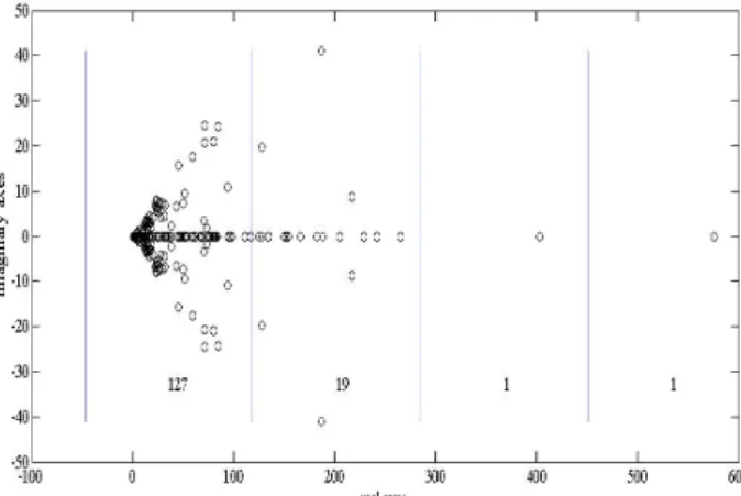
Fig. 1.The number of the eigenvalues for the Jacobean of the 118-bus test system in the first step of the Newton-Raphson algorithm. This graph is obtained using Alg. 2 for 5 slices.
C. Computing the Invariant Subspaces via MSF
MSF can be employed to compute a matrix whose eigenvalues are equal to the eigenvalues of matrix A in a specific range [7]. More technically,
Theorem 2.4: Let β∈ℜand matrix S is defined as: )) ( ( 2 1 I A sign I S= + −β (5)
By applying the rank revealing QR onto this matrix S, = Π 0 0 12 11 S S S QT
(6)
is obtained. Here, S11 is a kxk dimension matrix and k equals to the number of the eigenvalues of matrix A, which is bigger thanβ. The orthogonal matrix Q can be used for the transformation below. = = 22 12 11 0 ˆ A A A AQ Q A T
(7)
Finally, matrix A11 is a kxk matrix whose eigenvalues are equal to the eigenvalues of matrix A with real parts bigger than
β.
The same procedures in eigenvalue counting algorithm can be used to obtain the invariant subspaces in above theorem and we can compute different A11 matrices according to our
geometry selection in complex plane.
D. Building a Preconditioner with MSF
The preconditioners are used for accelerating the convergence of the iterative methods in linear equation system solution. The methods mainly aim to reduce the condition number of the coefficient matrices with several approaches. Basically the process can be summarized as reducing the groups of the eigenvalues of the coefficient matrix. According to Theorem 2.4 one can observe that MSF can also be useful for this purpose.
In suggested method, MSF is used in two different ways. In the first one, only the dominant eigenvalues of matrix A in a specified region of the complex plane are used to obtain a reduced condition numbered system. But in this way, the effect of the small eigenvalues on the condition number is neglected. Therefore, a second way is suggested to improve the method.
1)Type-I MSF Preconditioner: In the first type of MSF based preconditioner, only the dominant eigenvalues are considered. To achieve this information without computing eigenvalues Gerschgorin theorem is used. The Alg. 2 is used to obtain the brief information about the eigenvalue distributions and we take the desired percentage of the eigenvalues. There is no exact relationship between the percentage of the taken eigenvalues and the condition number in this case. In the second step, Theorem 2.4 is used to determine the transformation matrices Qb. Finally, the preconditioner matrix Mb is created as a combination of an identity matrix and A11
matrices as given below:
= −k n b I A M 0 0 11
(8) where A11 is a kxk matrix and In-k is an (n-k)x(n-k) identity
matrix. A11, contains exactly the eigenvalues of matrix A
bigger than the pre-selected valueβ. Then these matrices applied onto the linear equation set Ax=b as follows;
Mb−1QbTAQb(QbTx)=Mb−1QbTb (9) In (9), the matrix Qb is applied to A to change the order the
eigenvalues of A as the same as the preconditioner matrix Mb.
The other multiplication aims to preserve the structure of the linear equation system. At last Ax=b equation set is transformed into Anxn=bn where,
An =Mb−1QTbAQb b Q M bn= b−1 Tb x Q xn = bT
(10)
The new preconditioned equation set can be used to find the solution of the linear equation system. The algorithm of the Type-I MSF based preconditioner is given in Alg.3.
Algorithm 3 TYPE-I MSF BASED PRECONDITIONER Input : Matrix A, right hand side vector b, number of slices d
Output : Solution of the preconditioned linear equation set 1. Use Alg. 2 to computeβ.
2. Use Theorem 2.4 to compute A11 and Qb.
3. Build Mb matrices according to (8).
4. Compute An and bn according to (10).
5. Use An and bn to obtain xn in GMRES algorithm. 6. Compute the real x as x=Qbxn.
2) Type-II MSF Preconditioner: The approximate condition number of a non-symmetric matrix is given as the ratio of the maximal singular value of the matrix to the minimal singular value. In Type-I MSF preconditioner we only dealt with the maximal eigenvalues. But it is not enough to achieve rapid solutions. Although there is no direct (only approximate) relation between the eigenvalues of a non-symmetric matrix and its condition number, we try to vanish the effect of the smaller eigenvalues in second type preconditioner. Here, in type-II MSF preconditioner design, eigenvalues of the matrix A with real part smaller than 1 are also considered.
Fig. 2. Eigenvalue distribution of the Jacobean matrix and the preconditioned matrix with Type-I MSF in histogram mode. Here, 118 bus system is used as an example. Eigenvalues of the Jacobean matrix are located in seven different groups in complex plane. On the other hand eigenvalues of the preconditioned Jacobean matrix are located in just three different groups.
To obtain the preconditioner, theorem 2.4 can be implemented in a different way as;
Theorem 2.5: Let α∈ℜand matrix S is defined as: )) ( ( 2 1 I A sign I S= − −α (11)
By applying the rank revealing QR onto this matrix S, = Π 0 0 12 11 S S S QT
(12)
is be obtained. Here, S11 is a kxk dimension matrix and k is equal to the number of the eigenvalues of the matrix A, which are smaller thanα . The orthogonal matrix Q can be used for the transformation below.
= = 22 12 11 0 ˆ A A A AQ Q A T
(13)
Finally, matrix A11 is a kxk matrix whose eigenvalues are equal to the eigenvalues of the matrix A with real parts smaller than theα.
If we select α=1in theorem 2.5, we can obtain the orthonormal matrix Qa and A11 matrix which preserves the
eigenvalues of the matrix A, which are smaller than 1. After applying this theorem we can apply the Alg.3 first, then we have two steps algorithm to obtain the new equation set. The algorithm of this approach is given in Alg. 4.
To show the efficiency of the improvement, IEEE 118 bus test case is used. The parameter α for Type-II algorithm is selected as a constant value and different values are selected for β value for both types of algorithms. Then, the change of the estimated condition number is observed. Here, α =1.1and
βis changed from 50 to 500.
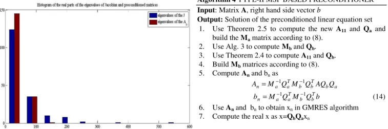
Algorithm 4 TYPE-II MSF BASED PRECONDITIONER Input: Matrix A, right hand side vector b
Output: Solution of the preconditioned linear equation set 1. Use Theorem 2.5 to compute the new A11 and Qa and
build the Ma matrix according to (8).
2. Use Alg. 3 to computeMb and Qb.
3. Use Theorem 2.4 to compute A11 and Qb.
4. Build Mb matrices according to (8).
5. Compute An and bn as a b T b b T a a n M Q M Q AQ Q A = −1 −1 b Q M Q M bn = a−1 aT b−1 bT
(14) 6. Use An and bn to obtain xn in GMRES algorithm
7. Compute the real x as x=QbQaxn
Fig. 3. Comparison of the condition numbers of preconditioned matrices with different β values for both types of algorithms. It can be easily seen from the figures that IEEE 118 bus test system has better condition numbers after type-II preconditioner is applied even for bigger βvalues.
III. NUMERICAL RESULTS A. Comparison of MSF-based Methods
Some popular and well-known IEEE power system test cases are used for the tests. In every step of the Newton-Raphson algorithm a Jacobean matrix is created. We used the first Jacobean in our tests. It is proved that the eigenvalue spectrum of the Jacobean in different steps does not vary dramatically. The main advantage of the suggested algorithm is based on this observation. The preconditioner matrix is created in the very beginning of the algorithm and then it is used for different Jacobeans. The main mathematical properties of the test cases are given in Table 1.
There are two types of implementations for MSF-based preconditioners. In the first case, one can take only the dominant eigenvalues of matrix A to obtain the transformation matrices. Mainly the approximate condition number of a square matrix can be defined as the ratio of the maximum and minimum singular values of a matrix. Therefore, the first type of MSF-based methods has not much effect on the condition number of the preconditioned matrix. To improve the method, one can select the eigenvalues whose real part is smaller than 1
and the dominant ones. Thereby, both the biggest and the smallest parts of the spectrum are vanished. According to approximate condition number definition given above, the condition number of the preconditioned matrix will be decreased if we apply the second type of MSF-based method.
TABLEI
NUMERICAL PROPERTIES OF IEEETEST CASES
In the first test, IEEE 57 bus test case is used and the parameter αis selected as constant and the parameter βis varied from 110 to 20. In this case, it is observed that the iteration number for GMRES to achieve a desired accuracy is getting better for both types of preconditioners. On the other hand, type-II preconditioner gives more satisfactory results. In all tests we choose a default tolerance as tol=10-16. The results are given in Fig. 4.
B. Comparison between ILU and MSF-based methods
The same power flow data are used for the comparison of the most widely used preconditioning technique, Incomplete LU (ILU), and the MSF-based methods. ILU methods produce an approximation for the classical LU decomposition and these incomplete L and U are used as preconditioner [5]. ILU factorization has several types.
Fig. 4. Required iteration numbers for convergence for different β. Obviously, in both method if the eigenvalue numbers increase the iteration number will be decreased. But in Type-II preconditioner, even for larger β values (in other words smaller eigenvalue numbers) gives better results.
1. ILU-Threshold: The entries of L and U matrices below some threshold value are discarded and the resultant factors are used as preconditioners.
2. ILU('x'): Dropping of fill-ins are decided by the sparsity pattern of matrix A. For example in ILU(0) means there is no permission for the fill-ins outside the sparsity pattern of matrix A.
The changes of condition number of preconditioned matrices for different types of preconditioners are given in Table 2. In all cases the first Jacobean of the system is considered only. Built-in Matlab function for Incomplete-LU factorization is used in all tests.
TABLEII
COMPARISON OF CONDITION NUMBERS FOR DIFFERENT PRECONDITIONED
MATRICES
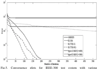
In the second test, the convergence graphs of ILU preconditioners and type-II preconditioner are compared with two different β values 600 and 300. For β=300, the number of eigenvalues used to form the preconditioner is 90. On the other hand, in β=600 case 50 eigenvalues are used. The convergence plots for these cases can be seen from the Fig. 5.
Finally, the Type-II MSF is used as a preconditioner in the Newton-Raphson iteration of power flow simulation. To do this, Matpower package is used [10]. In Matpower package, the default solver is classical LU method. To test our preconditioner, the solver is changed with GMRES obtained from the templates of NETLIB [11]. In our test we used 118 and 300 buses classical IEEE examples, important properties of which are given in Table 1.
Fig.5. Convergence plots for IEEE-300 test system with various preconditioner.
Two different βvalues for Type-II MSF preconditioner are selected for each case. The preconditioner matrix is created only once and it used in all other Newton-Raphson steps. For IEEE-300 test case, we observed that, GMRES with ILU(0) does not converge to the correct value. As a result one can say that satisfactory acceleration with type-II preconditioner is obtained. To improve the computational efficiency for type-II preconditioner, some code optimization techniques and parallel implementation has to be considered.
TABLEIII
ITERATION NUMBER IN EACH NEWTON-RAPHSON STEP FOR THE TEST CASE IEEE-118
TABLEIV
ITERATION NUMBER IN EACH NEWTON-RAPHSON STEP FOR THE TEST CASE IEEE–300
IV. CONCLUSION
In this study, we suggest a new preconditioner design for the iterative solution of the linear equation systems arising from the power flow simulations. Although direct methods with sparse techniques are very common in the area of power system simulation, these types of methods are not suitable for parallel processing. On the other hand, if the system size is getting bigger, parallelism is a must for fast simulations. Therefore, iterative methods have to be considered in the area of power system simulations. But most of the times, iterative methods need preconditioners to accelerate the convergence. A new preconditioner based on the Matrix Sign Function (MSF) is suggested in this work. The main idea is vanishing the extreme eigenvalues to reduce the number of eigenvalue groups. To do this, spectral division properties of the MSF is employed. The main computational cost of the design of suggested preconditioner is computation of the MSF. Meanwhile some well-known computational tools like QR decomposition also increase the computational cost of the design. On the other hand, these computations are done only once. The same preconditioner can be used in subsequent Newton-Raphson iterations. From this point of view, our algorithm has an advantage against the well-known preconditioner, Incomplete LU. The suggested preconditioner has a block structure. Therefore, it is suitable for parallel processing. In our future work, we plan to improve the computational efficiency of the method and implement it on parallel architectures with more realistic examples.
V. REFERENCES
[1] H. Dag, A. Semlyen, "A New Preconditioned Conjugate Gradient Power Flow ", IEEE Trans. Power Systems, Vol:18, No:4, pp:1248- 1255, 2003.
[2] R. Freund, G. Golub, N. Nachtigal, "Iterative solution of linear systems ", Acta Numerica, pp:57-100 Cambridge, U.K., Cambridge University Press, 1991.
[3] G. Golub, C. Van Loan, "Matrix Computations”, The John Hopkins University Press, 1996.
[4] H. Dag, F. L. Alvarado, "Computation-free preconditioners for the parallel solution of the power system problems”, IEEE Trans. Power Systems, Vol:12, No:2, pp:585-591, 1997.
[5] K. Chen, "Matrix preconditioning techniques and applications", Cambridge University Press, 2005.
[6] N. J. Higham, "Functions of matrices, theory and computation", SIAM Publishing, 2008.
[7] Z. Bai, J. Demmel, "Design of a parallel non-symmetric eigenroutine toolbox, part 1", Technical Report, UCB/CSD-92-718, UC Berkeley, 1992.
[8] P. Benner, E. S. Quintana-Orti, "Model reduction based on spectral projection methods", Dimension Reduction of Large-Scale Systems, pp:5-48, Lec. Notes in Comp. Sci. and Eng. Vol:45, 2006.
[9] E. F. Yetkin, H. Dag, "Applications of Eigenvalue Inclusion Theorems in Model Order Reduction", Scientific Computing in Electrical Engineering, SCEE 2008, Espoo, Finland, 2008.
[10] R. D. Zimmerman, C. E. Murillo-Sánchez, and R. J. Thomas,"MATPOWER's Extensible Optimal Power Flow Architecture,"Power and Energy Society General Meeting, 2009 IEEE, pp. 1-7, July 26-30 2009.
[11] R. Barrett, M. Berry, T. F. Chan, J. Demmel, J. Donato, J. Dongarra, V. Eijkhout, R. Pozo, C. Romine, H. Van der Vorst, Templates for the Solution of Linear Systems: Building Blocks for Iterative Methods, 2nd Edition, SIAM Publishing, 1994.
VI. BIOGRAPHIES
Hasan Dağ(M’90) received the B. Sc. degree in electrical engineering from Istanbul Technical University, Turkey and the M. Sc. and Ph. D. degrees in electrical engineering from the University of Wisconsin-Madison. Currently, he is a professor at the Information Technologies Department, Kadir Has University, Turkey. Also he is a board member of the National Center for High Performance Computing of Turkey. His main interests include the analysis of large scale power systems, the use of iterative methods and parallel computation.
E. Fatih Yetkin received the B. Sc. degree in electronics engineering from Uludağ University Turkey and M. Sc. in Computational Science and Engineering from Istanbul Technical University, Turkey. He is currently a Ph. D. student in Computational Science and Engineering department in same university. His main research interests are model order reduction, iterative methods and parallel computing.