Power Consumption Estimation using In-Memory Database Computation

Power Consumption Estimation using In-Memory

Database Computation

Hasan Dag

Management Infonnation Systems Department Kadir Has University, Istanbul, Turkey

Email: hasan.dag@khas.edu.tr

Abstract-In order to efficiently predict electricity consump­ tion, we need to improve both the speed and the reliability of computational environment. Concerning the speed, we use in­ memory database, which is taught to be the best solution that allows manipulating data many times faster than the hard disk. For reliability, we use machine learning algorithms. Since the model performance and accuracy may vary depending on data each time, we test many algorithms and select the best one.

In this study, we use SmartMeter Energy Consumption Data in London Households to predict electricity consumption using machine learning algorithms written in Python programming lan­ guage and in-memory database computation package, Aerospike. The test results show that the best algorithm for our data set is Bagging algorithm. We also emphatically prove that R-squared may not always be a good test to choose the best algorithm.

Index Terms-In-Memory Database, Machine Learning, Power

Consumption.

I. INTRODUCTION

The world of technology is growing every day. The devel­ opment of both software and hardware along with the increase in infonnation creation and sharing of all structures and sizes have engendered the Big Data era [1]. The need for processing large data fast enough for decision-making has increased the need for new solutions, capable of facing this dilemma. Today, machines create all sorts of data and share them with other machines. For companies, processing data is a priority. The companies that succeed in the analysis and processing of data to take the right strategic decision have fewer risks of failure. The capacities of storage have increased enormously lately. However, the usage of hard disk (HD) is not fast enough in the era of big data. When dealing with large data sets, HD or solid state drives (SDD) do not accompany the speed of new processors. HD is slow and fails to respond timely to all requests done daily basis. One of the best solutions is to use the in-memory databases. The advantage of using in-memory over HD is that there will be no latency between the hard disk and RAM.

Companies from different sectors including the energy have been investing in data analysis for many reasons. In fact, there are many companies specialized in electricity manage­ ment offering help and assistance for electricity consumption management, based on big data analysis. Their process starts by observing and collecting information on the general con­ sumption of a certain company, in order to understand the

978-1-5090-3784-1/16/$31.00 ©2016 IEEE

Mohamed Alamin

Management Information Systems Department Kadir Has University, Istanbul, Turkey

Email: ben_alamine@yahoo.com

electricity consumption cycle and therefore propose different solutions to decrease the consumption. Actually, the need of power consumption increases due to the independence on the electrical devices and technologies in businesses [2]. As for big companies, the high prices of power consumption impose the control and the management of the overall electricity usage. Even though multiple sources of energy are available, they are still expensive and not all of them are applicable especially for companies that use electricity in a massive way.

Using machine learning algorithms and past data, we can determine the peak hours and estimate the consumption in future for a better management of the energy resources. Generally, the prices of the electricity depend on time; the electricity is always more expensive in peak times. In order to avert the need of using more generators, it is essential to try decreasing the consumption in those peak hours. For example, by turning off the unnecessary lights or the heating and cooling systems during these periods.

In this study, we make use of in-memory databases [3] to predict future demand using real data and machine learning algorithms. since they represent the future of fast data pro­ cessing.

The rest of the paper is as follows. Section 2 briefly dis­ cusses electricity demand management, Section 3 discusses the in-memory databases and computation whereas section 4 deals shortly with machine learning techniques. We discuss in detail both the results and application of in-memory computation techniques on real data set using machine learning algorithms in Section 5. The conclusions are then provided.

II. ELECTRICITY DEMAND SIDE MANAGEMENT

Nowadays, utilities have a tendency to invest in Demand Side Management (DSM) for many reasons. In fact, it became important to manage and control the energy usage in order to reduce costs related to the power consumption and the power generation resources. The growth in population and the extensive usage of electronic devices led to an increase in power usage and consequently created the need for further resources. The utilities today seek a way to achieve their goals with lower costs. The electricity DSM offers solutions for a better management of electricity consumption based on the future prediction of the electricity usage. According to a report from Navigant Research, the global spending on

DSM will increase from $214.7 million in 2015 to $2.5 billion in 2024 [4]. The implementation of smart meters is a widely used technique to collect electrical data from the devices on a big scale. This data is analyzed to determine the pattern of electrical loads which allows a future prediction of the electricity needs and therefore be prepared for the peak times. DSM proposes different solutions for the electricity management in order to avoid the waste of energy and the need for new power installations. Companies that use electricity on a large scale are the most interested in DSM since it offers solutions enabling one to decrease the costs of electricity usage and reduce the risks related to the critical needs of extra power generators.

III. IN-MEMORY COMPUTATION

In the last few years, the In-Memory Technology has been used at a large scale in many fields. Big companies, in particular, have shown a lot of interest towards In-Memory technologies, ever since the need for fast data processing has increased dramatically. With the impact of the Big Data era, there is a greater need of processing data at a larger scale and fast enough for a real-time or a near real time response. The need of new technologies that can process data quickly has become a necessity. In-Memory database (IMDB) or Main Memory database (MMDB) is a database that stores data in the main memory (RAM). In conventional databases, the data goes from HD to RAM, and then it is processed by the processor, i.e., cpu. However, within the IMDB, the data will reside in RAM instead of HD. This means that the data would take a short cut directly from RAM to be processed.

The IMDB contains two main parts: the Main Store and the Buffer store. It has also a backup system on the hard disk or the SSD of flash memory to restore data if the system crashes; that is called the Durability Store. In addition, it has one or more types of data structure store (key value) and indexes. Using IMDB can provide many benefits, especially speed. The stream of data when using IMDB decreases in size. The main memory can present a solution since it is by nature faster than the hard disk. The index structure of the hard disk aims to minimize both the number of disk accesses and the disk space; whereas the index structure of the main memory doesn't need to minimize any disk accesses since it is contained in main memory. However, the implementation of a solution based on RAM is a challenging operation. Each memory has its own specifics. To start with, LO the register is the smallest one, but it is also the fastest. The latency time or the response time from first layer Ll cached data word is 0.5 nanoseconds. However, it can only hold one word. The second layer, L2 holds one line and it delays 7 nanoseconds, the delayed time from the main memory to the registry is about 100 nanoseconds (0.1 Microseconds), Solid state drive SSD takes 150 microseconds

(150,000 nanoseconds) such as in Fig. 1.

On the other hand, the hard disk drive takes about 10 milliseconds (150,000,000). As we can see, the difference between HDD and SSD is about 9,750,000 nanoseconds. For this reason, many computer companies started to use the SSD

Fig. 1. Memory Hierarchy [5].

instead of HDD. However, there is still not enough processors to process a large amount of data in a short time. Hence, there is no way to compare between the HDD and the Main memory in terms of speed. Still, the main memory is small and more expensive compared to the HDD. These technologies were used widely and developed constantly in the mid of 2000s due to the increasing capacity of data storage. The dropping prices of these technologies have encouraged the companies to obtain and invest in the in-memory technology. To illustrate this fact, in the late 1990s 1 gigabyte of main memory used to cost about a 1000-dollar. Today, you can get the same 1 gigabyte for less than 5 dollars, as shown in Fig. 2.

Action

L 1 cache reference (cached data word) Branch mispredict

L2 cache reference Mutex lock/unlock Main memory reference Send 2,000 byte over I Gb/s network SSD random read

Read I MB sequentially from memory Disk seek

Send packet CA to Netherlands to CA

Time (ns) 0.5 25 100 20.000 150,000 250.000 10.000,000 150.000.000

Fig. 2. Latency numbers [6].

IV. MACHINE LEARNING

Time 0.1 �s 20�s 150�s 250�s IOms 150ms

In order to define what machine learning is; it is important to understand to what each word refers. Machine learning is composed of two notions: machine and learning. The machine is the subject of the process, it must learn and develop itself, and that is from where learning comes.

Actually, learning means changing the behavior with expe­ rience. In machines, learning involves the amelioration of pre­ diction based on changes in data or the program. Tom Mitchell gave the following definition when asked about machine learning: A computer program is said to learn from experience E with respect to some task T and some performance measure P, if its performance on T, as measured by P, improves with experience E.

The machine observes the first data and makes a prediction, but when exposed to new data, it gives a better prediction. That is the process of learning.

Machine learning involves developing programs to learn in order to improve then performance every time exposed to new data. It has a goal of solving a problem based on past knowledge.

Machine learning is a subfield and an essential part of Artificial Intelligence for the simple fact that there could not be any artificial intelligence machine without machine learning. There are many reasons that made machine learning important today:

* The development of new technologies and the interest of

artificial intelligence.

* Big data and the large sizes of data are created every day

from different sources.

* The need for speed in analyses processing and less human

involvements.

* The machine can extract and remember information that

is hidden or non-logical to human thinking.

Machine learning is based on many disciplines, which are statistics, psychology (copy the human brain), biology (neural network) and computer science.

There are some important concepts in machine learning, such as the generalization. It means that the machine learns something for data, and develops a general idea based on the examples. This generalization allows prediction of the new examples. The other important concepts are the training and testing. The algorithms learn first form the training data and develop a model that fits this data. To evaluate the algorithm, we use the test set.

Different algorithms can be used to solve a machine­ learning problem. In genera\, the choice of the algorithms depends on the type of the data and the type of the problem that needs to be treated. There are algorithms for regression, clustering, and classification.

V. SMARTMETER ENERGY CONSUMPTION DATA IN

LONDON HOUSEHOLDS DATA SET

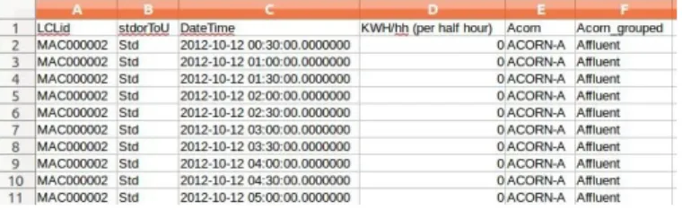
In this study, we use a sample of the energy consumption readings that contain 4,376 London Households in the UK, within the period of November 2011 and February 2014 [7].

The consumption is measured in kWh for every 30 minutes. The features include an ID of the households, the date and time, and CACI Acorn group. The total size of the data set is 11 gigabytes, which is around 167 million rows. A sample is provided in Fig.3.

A. Why London Households Data set?

Our choice is based on the fact that the data set represents the real data of electricity consumed by real people in their houses. Unlike the electricity consumption data of factories or malls - which have approximately the same value every day- this data represents the inconsistency and diversity in the electricity consumption of people depending on their life style and habits, such as the time spent inside the house, late parties,

Fig. 3. Sample of SmartMeter energy consumption data set.

usage of electrical gadgets, etc. In addition, some people use their house only during the summer holidays or weekends. B. Preprocessing Data set

We need to preprocess our data to eliminate the unwanted or redundant data [8], make corrections, deal with missing values, and prepare it for the analysis. To this end, we apply the following preprocessing steps:

• Feature reduction: We deleted some columns that have

the same values and never change like, Acorn and Acorn grouped.

• Delete Null Values: Every house that has one or more

null values of power and non-hourly time, is eliminated.

• Separate DateTime column: We divided the DataTime

column to six columns in order to use them in the comparison and make every column as a variable that can affect the result of prediction.

• Id of House: We changed the ID of houses from string

values to integer values, in order to use the ID in most of the machine learning models. In addition, we changed the power consumption from KW to Watts.

• Delete incomplete data: Not all the houses have full

region data covering the entire period from November 2011 until February 2014. For example, house number 1957 contains only data from 11-06-2012 till 26-6-2012, which is less than one month. We delete this type of houses. As a result, we have a total of 4,130 houses to work with.

• Add days: We add the days feature to make our predic­

tion more accurate. As we know, by adding weekdays and weekends we can determine the reasons behind the changes in power consumption based on the days. For example, the difference between the consumption in Sundays and Mondays is noticeable. This operation has increased the prediction value by approximately 10% in some houses. A snapshot of the data after cleaning is given in Fig. 4.

• Half-hourly to Hourly: We change the data from half

hourly to hourly power consumption as in Fig. 4. This would reduce our data to half and improve the prediction. The total size of the data is now 4150 houses with l.6 Gigabyte.

• Shape the data: Figure 5 show the consumption for an

house just for one day, 28-4-2012. we can determine in which hours the power consumption is higher. As we see, the costumer consumes more power between 11 am and

Fig. 4. Sample of data set after preprocessing.

15 pm, and the highest period is between 18pm and 22 pm in the evening. Furthermore, the period of time when the costumer doesn't consume much power is between 2 and 7 am.

Fig. 5. Electricity consumption for one day for one house.

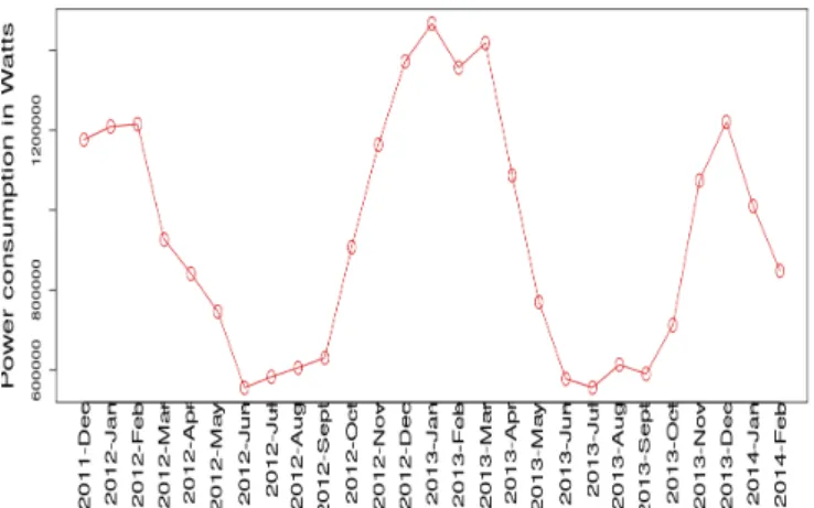
Figure 6 depicts monthly power consumption data of house number 145. We can understand the months where the users consume more power, in this case it is in December, January, and February, which can be explained by the weather con­ dition. Also there is small increase in June, which may be caused by the usage of the air conditioner.

Fig. 6. Total electricity consumption based on months.

VI. CHOICE OF T HE BEST MODEL OF MACHINE LEARNING

TO FIT OUR DATA

First, we want to choose some models, to apply them and determine which model can fit all or most of our data and

give good results. We did a comparison of some models using different machine learning tools. But first, we split data to training and testing sets.

The split is done using a library called (train test split) in python to split the data to a training data and a testing data. The value that was given for data training is 80 percent and for testing 20 percent. First, we chose five regression models: Random Forest, Decision Tree regression, Extra Tree regression, Bagging regression and Linear regression. A. First Test (R-squared, R2)

We used R2 to test the different models and chose the best one.

The R2, also called the coefficient of determination is a statistical method used for many regression and statistical analysis and is most commonly used to determine the quality of a statistical models fit [9]. The R2 error value generally varies from 0 to 1. The model is considered to be a good fit if its R2 value is close to 1. The formula of the R2 error is: (1) where the SSE represents the sum of squared errors and the SST stands for the total sum of squares [10].

First we applied it to house number 3. We can see the results in Table I. We obtained the best results from the Bagging regression (0.896) and the Random forest (0.895) methods for the house number 3 as shown in Table I. While replicating

TABLE I

R2 RESULTS FOR VARIOUS ALGORITHMS USING HOUSE 3 DATA.

Algorithm RL Bagging regression 0.896080196574 Random regression 0.895494830121 Extra regression 0.87848854631 Decision regression 0.376203098132 Linear regression 0.209074906098 k nearest neighbors 0.691809565284

the same calculation on the house number 1199 as seen in Table II, the R2 results were not good. For this house, R2 calculation for Bagging was -0.005, R2 for Random Forest was -0.053 but with Decision tree it was 0.10.

TABLE II

R2 RESULTS FOR VARIOUS ALGORITHMS USING HOUSE 1199 DATA.

Algorithm RL Bagging regression -0.00505593237186 Random regression 0.0533046674133 Extra regression -0.0604631321477 Decision regression 0.108030788443 Linear regression 0.0350849871945 k nearest neighbors 0.0425716922033

B. Second Test (Summation of months)

In this test we calculated the summation of every month independently for testing purpose. The results divided by the sUlmnation of the predicted data.

As presented in the house number 3 in Fig. 7, we can see the line fits perfectly with Bagging and Extra regression and lost in some points with Random Forest. But the Decision tree and Knn didnt fit exactly, yet they follow the same curve but do not fit the points.

Fig. 7. Comparison of ML algorithms for monthly electricity consumption for house number 3.

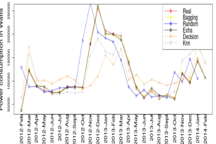
Fig. 8. Comparison of ML algorithms for monthly electricity consumption for house number 1199.

In house number 1199 as shown in Fig. 8, the R2 value was negative. However, we can see that there was no model that fitted the curve of real value. Yet, we can see that at some points, the Bagging and the Random Forest models were good fits, as in June and December 2012 and March, April and September in 2013. this result led us to elaborate another test.

C. T hird Test (By differences between real and predicted individual data)

We conducted another test by calculating the differences between the real data of the test set and the predicted data. This test includes the calculation of the difference between the first value of the test set and the first value of the prediction, then the difference between the second value of the test set and the second value of the prediction, and so on. At the end, we sum up the differences and divide it by the summation of the real values of the test set.

where:

P

ifsum(abs(P - P))

sum(P) :

(2)

result

abs(sum(abs(P - P))jsum(P)

)

else:

result

abs( sum( abs( P - P)) j sum( P))

The results of this test were different than the result of the R-squared. For house number 3 as seen in table III, using Bagging, the results of (differences between data test and predicted data) are 0.73 for Bagging and 0.72 for Random Forest. We notice that the results are less than the R-squared calculated values. However, the house 1199 as seen in Table IV showed a completely different and interesting results. The Bagging and Random got 0.38 although R2 was equal to -0.005. But for the Decision Tree the result was 0.4.

In fact, house 3 and house 1199 are different. House 3 represents a decent house with a regular and ordinary power consumption. On the other hand, house 1199 is characterized by the irregularity in the power consumption, which may have confused the R2 calculation to give a negative output.

Since R2 may in some cases give inconclusive values, we decided to perform more tests.

TABLE III

COMPARISON OF ALGORITHMS FOR HOUSE 3.

Algorithm R" Differences Bagging regression 0.896080196574 0.730565101844 Random regression 0.895494830121 0.721535570183 Extra regression 0.87848854631 0.715903642935 Decision regression 0.376203098132 0.333302025741 Linear regression 0.209074906098 0.139211611706 k nearest neighbors 0.691809565284 0.551830094765

D. Fourth Test (Choose 500 houses randomly)

We calculated the average of R2 and the differences for 500 houses selected randomly as seen in Table V. We can see that all results of R2 are less than 0.43. But using the

TABLE IV

COMPARISON OF ALGORITHMS FOR HOUSE 1199.

Algorithm R" Differences Bagging regression -0.00505593237186 0.388482137428 Random regression 0.0533046674133 0.381369335206 Extra regression -0.0604631321477 0.370511945392 Decision regression 0.108030788443 0.401667363226 Linear regression 0.0350849871945 0.353074466826 k nearest neighbors 0.0425716922033 0.383886275354

differences formula, the Random forest and Bagging result in a higher vaLue of 0.61. Extra regression got 0.60 and K Nearest Neighbors with 0.58. Linear regression value equals 0.44 (although Linear got 0.12 using R-squared).

TABLE V

R2 AND DIFFERENCE OF 500 HOUSES RANDOMLY

Algorithm R" Differences Bagging regression 0.421451144778 0.614139562817 Random regression 0.421121406344 0.614143242967 Extra regression 0.388489691547 0.605980602049 Decision regression 0.212188577625 0.495803420023 Linear regression 0.125578016697 0.447913538955 k nearest neighbors 0.382293658572 0.580228344575

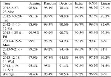
E. Test Five (Predict determined hour for All Houses) In this test, we chose some hours from different days. We selected 8 hours randomly from the data. This test consists of dividing the sum of the predicted data at those specific hours by the sum of the reaL data at those same hours. The results can be understood clearly from the (TabLe VI). As we can see, there is no difference between Bagging and Random Forest. However, the best result belongs to Extra tree regression and the worst model is the Linear Regression. Those are small difference, but with thousands of houses, the effect can be big.

TABLE VI

PERCENTAGE PREDICTION FOR DETERMINED DATE TIME OF ALL HOUSES

Time Bagging Random Decision Extra KNN Linear

2012-2-27- 98.8% 98.1% 78.4% 98.5% 98.291 78.1% 23-Mon 2012-7-3-20- 99.1% 98.9% 98.8% 99.7% 97.591 98.3% Tue 2012-11-10- 98.9% 99.3% 90.6% 99.7% 99.691 82.6% 12-Sat 2013-1-25-6- 99.98% 99.9% 90.7% 99.5% 95.491 92.3% Fri 2013-4-15-5- 99% 98.8% 94.9% 99.7% 99% 89% Mon 2013-9-21-1- 99.2% 99.2% 84.4% 99.5% 97.891 81% Sat 2013-12-18- 97.9% 97.8% 94.8% 98.9% 97.291 99.2% 14-Wed 2014-1-19- 95.4% 95% 91.4% 97.8% 90.791 91.5% 14-Sun Average 98.4% 98.4% 90.5% 99.2% 96.991 89% VII. CONCLUSION

This study, to the knowLedge of the authors, is the first application of machine learning using in-memory database. We use the Aerospike as the in-memory database and use the SmartMeter Energy Consumption Data in London Households data set. We applied many machine learning algorithms for prediction, before selecting the best one: The Bagging Algo­ rithm. During the process, we demonstrated that R-squared error is not always the best indicator for success of the algorithms The usage of main memory is expected to be more and more important in the future. The limitation of I/O delays is opening doors to more researchers to develop this technoLogy. Most of the smart grid applications, if not all, that need real-time response, or near-reaL-time response are expected to start using the main memory instead of HDD.

REFERENCES

[II M. Swan, "Philosophy of big data expanding the human-data relation with big data science services," IEEE First International Conference on Big Data Computing Service and Applications, 2015.

[21 L. Tan and N. Wang, "Future internet: The internet of things," 3rd International Conference on Advanced Computer Theory and Engineer­ ing(ICACTE), 2010.

[31 M. K. Gupta, V. Verma, and M. S. Verma, "In-memory database systems - a paradigm shift," nternational Journal of Engineering Trends and Technology (!JETT), vol. 6, Dec. 2013.

[4] Behavioral and analytical demand-side management spending is expected to reach $2.5 billion in 2024. [Online]. Available: https:llwww.navigantresearch.com/newsroomlbehavioral-and-analytical­ demand-side management-spending-is-expected-to-reach-2-5-billion-in-2024.

[5] The memory hierarchy. [Online]. Available:

http://blog.csdn.net/cinmyheart/articIe/details/36687963

[6] H. Plattner, A Course in In-Memory Data Management, 2nd ed. German: Springer, 2014.

[7] Smartmeter energy consumption data in london households. [On­ line]. Available: http://data.Jondon.gov.uk/dataset/smartmeter-energy-use­ data-in-Iondon-households.

[8] S. B. Kotsiantis, D. Kanellopoulos, and P. E. Pintelas, "Data preprocessing for supervised leaning," International Journal of Computer, Electrical, Automation, Control and Information Engineering, vol. 12, 2007. [9] N. 1. D. NAGELKERKE, "A note on a general definition of the coefficient

of determination," Oxford University Press on behalf of Biometrika Trust, vol. 72, pp. 691-692, Sep 1991.

[l0] R squared. [Online]. Available:

http://www.hedgefund-index.comld_rsquared.asp

[11] F. Dubosson, S. Bromuri, and M. Schumacher, "A python framework for exhaustive machine learning algorithms and features evaluations," IEEE 30th International Conference on Advanced Information Networking and Applications, 2016.