1877–0428 © 2011 Published by Elsevier Ltd. doi:10.1016/j.sbspro.2011.04.525
Procedia Social and Behavioral Sciences 17 (2011) 416–437
Social and
Behavioral
Sciences
Procedia - Social and Behavioral Sciences 00 (2010) 000–000www.elsevier.com/locate/procedia
19
thInternational Symposium on Transportation and Traffic Theory
Models for Relief Routing: Equity, Efficiency and Efficacy
Michael Huang
a, Karen Smilowitz
a*, Burcu Balcik
baIndustrial Engineering and Management Sciences, Northwestern University 2145 Sheridan Rd. Evanston IL 60208 USA bIndustrial Engineering Department,Kadir Has University, Cibali, Istanbul, Turkey 34083
Abstract
In humanitarian relief operations, vehicle routing and supply allocation decisions are critically important. Similar routing and allocation decisions are studied for commercial settings where efficiency, in terms of minimizing cost, is the primary objective. Humanitarian relief is complicated by the presence of multiple objectives beyond minimizing cost. Routing and allocation decisions should result in quick and sufficient distribution of relief supplies, with a focus on equitable service to all aid recipients. However, quantifying such goals can be challenging. In this paper, we define and formulate performance metrics in relief distribution. We focus on efficacy (i.e., the extent to which the goals of quick and sufficient distribution are met) and equity (i.e., the extent to which all recipients receive comparable service). We explore how efficiency, efficacy, and equity influence the structure of vehicle routes and the distribution of resources. We identify trends and routing principles for humanitarian relief based on the analytical properties of the resulting problems and a series of computational tests.
© 2009 Published by Elsevier Ltd.
Keywords: vehicle routing; supply allocation; equity; humanitarian relief
1. Introduction
Recent disasters have increased attention on the effectiveness of humanitarian aid; there is increased pressure from donors on relief agencies to show that pledged aid and goods are reaching those in need quickly (Van Wassenhove, 2006). This has led to a larger focus on improving humanitarian relief logistics. The recent large scale disasters and relief efforts (e.g., 2004 Asian tsunami, 2005 Pakistan earthquake, 2010 Haiti earthquake) highlight the need for improved logistics in the field. For example, following the Tsunami, the amount of pledged relief overwhelmed the relief agencies' ability to properly store and distribute the aid (Russell, 2005). Given the trends in the impact of disasters on vulnerable populations and economies worldwide and the criticality of logistics in humanitarian relief operations, it has been increasingly highlighted that Operations Research (OR) can help improve the logistics of humanitarian aid (Van Wassenhove, 2006).
This paper focuses on last-mile distribution in a humanitarian relief chain from a distribution center to beneficiaries (Balcik, Beamon, & Smilowitz, 2008). Relief supplies must be delivered quickly in sufficient amounts.
* Corresponding author. Tel.: 847-491-4693 ; fax: 847-491-8005
E-mail addresses: [email protected] (M. Huang)
[email protected] (K. Smilowitz) [email protected] (B. Balcik) © 2011
Open access under CC BY-NC-ND license.
Given limitations in transportation resources and relief supplies, and damaged infrastructure, it is challenging to plan last mile operations (Balcik et al., 2008). Distribution decisions are often made ad-hoc, which may lead to inefficient use of resources, slow response, and inadequate or inequitable relief deliveries.
The classical vehicle routing problem (VRP) minimizes total transportation costs; in humanitarian relief, one is primarily concerned with whether the routes are able to deliver the aid quickly. Focusing on relief response times, Campbell, Vandenbussche, & Hermann (2008) show that the choice of objective affects how aid is distributed. With alternative objectives of minimizing the last arrival time and minimizing the sum of arrival times, the authors demonstrate that superior service times may be achieved than those resulting from a traditional VRP objective. They show that minimizing total routing costs results in solutions with longer response times.
Equitable aid distribution among recipients is also a critical consideration in humanitarian relief (Beamon & Balcik, 2008). However, equity may be hard to define both in practice and for modeling purposes. In this paper, we characterize equity in terms of the disparity between service levels among aid recipients, where service levels are characterized by delivery speed and amount. Even so defined, it is not clear how equity should be modeled. Furthermore, it is not obvious how different and potentially conflicting objectives of equity, efficacy and efficiency affect the route structures in the relief context.
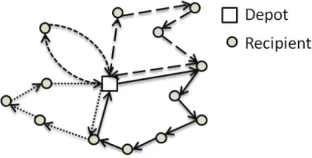
Balcik et al. (2008) present an analysis of last mile operations and show how modeling these operations with all the associated complexities can make it difficult to study the underlying differences in route design that occur. Our goal in this paper is to simplify the modeling of last mile distribution to a more stylized setting where we can more easily gain insights into the effects of equity and other considerations in relief distribution. We refer to this problem setting as the last-mile delivery problem (LMDP). The LMDP designs vehicle routes and distribution schedules for a fleet of vehicles delivering supplies from a distribution center, yet unlike Balcik et al. (2008), we focus on a single period problem where each vehicle performs at most one trip to deliver one commodity type. Although more restricted than Balcik et al. (2008), our problem setting still captures many critical characteristics of the last mile environment; in particular, the LMDP in this paper would well address relief operations in rural areas where each vehicle can perform only one trip per period and supplies are distributed in the form of standard packages/pallets. Relief organizations often make daily distribution plans rather than considering multiple days ahead, especially during the initial phases of the emergency due to the chaotic environment and lack of reliable information (Mantyvaara, personal communication, 2010). An example of LMDP routes is presented in Figure 1. The demand of a site can be satisfied by more than one vehicle in the LMDP, similar to the Split Delivery Vehicle Routing Problem (SDVRP). The SDVRP is motivated by the potential savings in costs due to splitting demand among multiple vehicles (Dror & Trudeau, 1989). Split deliveries in last mile relief distribution can allow one to quickly serve large demands using limited resources. Our problem setting allows us to analyze the impact of different objectives on route structures and the performance of aid distribution, in terms of (i) efficiency (transportation costs), (ii) efficacy (quick and adequate response), and (iii) equity (fairness as measured by deviations between recipients in efficacy). The incorporation of equity in particular leads to unique challenges.
Figure 1 A set of routes in LMDP
We develop a set partitioning model for the LMDP to incorporate alternative objectives, based on efficiency, efficacy and equity metrics. Analytical properties of the LMDP models are examined. A numerical study of small instances, in which it is possible to obtain optimal solutions for each of the objectives, is conducted to develop
insights into route characteristics. Our analysis shows that there exist substantial differences among solutions that attempt to minimize efficiency compared to those that are concerned with efficacy and equity. Heuristics are developed to solve large instances of the LMDP variations.
This paper is organized as follows: in Section 2, we review the relevant literature. Section 3 gives a detailed description and analysis of the LMDP variations. Section 4 proposes heuristics for the LMDP variations. Section 5 discusses practical implications of this work and future directions.
2. Literature Review
There is a growing literature that addresses relief supply distribution in humanitarian logistics. One of the earliest studies that addresses distribution of relief supplies from a distribution center to several camps is Knott (1987). The author formulates a linear programming model that finds the number of trips each vehicle makes to maximize the amount of deliveries while minimizing transportation costs and discusses how considering additional aspects might make the problem very difficult to solve. More recently, the literature addresses more complicated relief supply distribution problems and captures the inherent complexities of the humanitarian relief environment, including multiple commodities, multiple transportation modes or vehicle types, multiple periods, uncertain or varying demand and supply levels and transportation network conditions, and delivery time windows. Most studies develop heuristic algorithms to solve the proposed models (e.g., Haghani & Oh, 1996; Barbarosoglu, Ozdamar & Cevik, 2002; Ozdamar, Ekinci & Kucukyazici, 2004; Lin, Batta, Rogerson, Blatt & Flanigan, 2009; Shen, Dessouky & Ordonez, 2009; Van Hentenryck, Bent & Coffrin, 2010) or use commercial solvers to test the models for small to moderate problem instances (e.g., Barbarosoglu & Arda, 2004; Tzeng, Cheng & Huang, 2007; Balcik et al., 2008). Studies that focus on relief supply distribution consider a number of different objectives, including minimizing logistics costs (e.g., Haghani & Oh, 1996), minimizing the amount of unsatisfied demand (e.g., Ozdamar et al., 2004), and minimizing service completion or delays (e.g., Barbarosoglu et al., 2002; Yi & Ozdamar, 2007). Equity, although critical, is considered by only a few studies. Tzeng et al. (2007) consider fairness in the problem of choosing transfer point locations in distributing supplies from a set of supply points to demand points. A multi-period multi-objective model is developed that considers, in addition to minimizing total cost and travel time, fairness by maximizing the minimum service satisfaction among demand points. In Balcik et al. (2008), routing and supply allocation decisions are considered jointly in distributing multiple types of relief supplies. The authors minimize the maximum unsatisfied demand percentage over demand locations along a planning horizon. Delivery scheduling decisions are driven by costs due to supply allocation and transportation over multiple days. Lin et al. (2009) study a similar problem that considers delivery of prioritized items in a relief scenario; the authors develop a multiple objective model to minimize unsatisfied demand and travel costs and ensure equity.
Campbell et al. (2008) focus on service time and evaluate two objective functions: minimizing the maximum arrival time of supplies (minmax), and minimizing the sum of arrival times of supplies (minsum) - thereby minimizing the average arrival time. As each demand location is visited exactly once, and full satisfaction of demand is ensured, supply equity is not a concern in the study. The authors explore the impact of different objective functions. For the traveling salesman problem and the VRP, solutions obtained from minmax and minsum objectives are compared with solutions obtained by minimizing total travel time. It is shown that the minmax and minsum objectives ensure better response times for the demand locations, at the expense of reduced efficiency (i.e., increased total route length or costs). Our paper extends this work by considering demands at each recipient which necessitates alternate equity metrics.
Outside of humanitarian relief, equity-related issues have been widely studied using OR models in areas such as public facility location; see, for example, Erkut (1993), Mulligan (1991), and Marsh & Schilling (1994). Although routing decisions affect equitable service provision, most of the routing studies in the literature address only efficacy and efficiency objectives. In routing, equity-related issues have only recently received attention; and then, only limited to few applications mostly addressing public/nonprofit sector problems (see Balcik, Iravani, & Smilowitz, 2011). As stressed by Marsh & Schilling (1994), since there may not be a single equity metric for a specific application, analyses that explore the tradeoffs between equity and other objectives can be helpful in understanding the use of different equity policies and metrics. As such, this paper defines and formulates different equity metrics focusing on last mile operations in humanitarian relief.
3. LMDP Modeling and Analysis
This section describes the LMDP in further detail. Section 3.1 presents the general problem setting. Section 3.2 presents an integer programming formulation of the problem. Section 3.3 introduces the performance metrics for efficiency, efficacy and equity that define the LMDP model variations; Section 3.4 discusses analytical properties of the LMDP models. Section 3.5 presents a computational study of the different models.
3.1. Problem Setting
As mentioned earlier, the goal of this paper is to study a stylized version of the LMDP to gain insights into the underlying route structures. The LMDP is defined on a graph 𝐺 = (𝑵0, 𝑨) which we assume is complete and
symmetric. The node set 𝑵0 includes the depot (𝑖 = 0) and the demand locations (𝑖 ∈ 𝑵: 𝑖 = 1, ⋯ , 𝑁). Travel costs
(in hours), 𝑐𝑖𝑗 ∀ (𝑖, 𝑗) 𝜖 𝑨, are non-negative and satisfy the triangle inequality. Routes begin at time 𝑡 = 0. Demand
is measured in units of full pallets of relief supplies. Pallets are modeled as a single commodity, but each pallet may be composed of different types of supplies. The set 𝑲 = {1, ⋯ , 𝐾} represents a fleet of vehicles operating from the depot to serve the aid recipients and 𝐶 is the capacity of each vehicle measured in pallets. Demand may be split across multiple vehicles. We assume that the demand of any recipient is less than the capacity of a vehicle; 𝑑𝑖 ≤
𝐶 ∀ 𝑖 ∈ 𝑵 and sufficient supplies are accumulated at the depot which can be delivered to recipients (𝐾𝐶 ≥ ∑𝑖∈𝑵𝑑𝑖). Vehicles may complete at most one trip and thus a vehicle visits a node at most once and may not return to
the depot to refill its capacity.
The LMDP involves two types of decisions. Routing decisions determine for each vehicle a set of nodes and visit sequence (and hence the arrival times). Distribution decisions determine the number of pallets delivered at each visit. We develop performance metrics to measure the effects of these decisions and use the metrics as objective functions of different models of the LMDP. Efficiency (Z1) is measured by the total travel costs. Efficacy (Z2) is
measured by the sum of each pallet’s arrival time. Equity (Z3) is measured by several functions which capture the
disparity in efficacy among nodes.
3.2. Integer Program Formulation
The LMDP is formulated with an extension of the set partitioning formulation of the VRP. The set partitioning formulation of the VRP assumes that the set 𝑹 = {1, ⋯ , 𝑅} of feasible routes is given. Each route 𝑟 ∈ 𝑹 represents a set of nodes and an order in which the nodes are visited. From this information, the following parameters can be obtained for each route. The travel cost 𝑐𝑟 is the time required to travel the length of the route. The parameter 𝑏𝑖𝑟
denotes the presence of node 𝑖 on route 𝑟: 𝑏𝑖𝑟 = 1 if node 𝑖 is visited by route 𝑟, and 0 otherwise. The parameter 𝑎𝑖𝑟
denotes the arrival time at node 𝑖 on route 𝑟, if route 𝑟 visits node 𝑖 (i.e., 𝑏𝑖𝑟= 1). If route 𝑟 does not visit node 𝑖
(i.e., 𝑏𝑖𝑟= 0), 𝑎𝑖𝑟 equals 𝑇, an upper bound on the time horizon.
We assume that each candidate route in 𝑹 is performed by at most one vehicle. In Section 3.4, we show that there exists an optimal solution where each route is run at most once. The binary decision variables 𝑥𝑟 determine whether
route 𝑟 is selected; 𝑥𝑟= 1 if route 𝑟 is selected, and 0 otherwise. The integer decision variables 𝑦𝑖𝑟 indicate the
number of pallets delivered to node 𝑖 by route 𝑟.
We define the LMDP(Zf) as the model of the LMDP with the objective function of minimizing the generic metric
Min Zf(𝑥, 𝑦) (1a) subject to ∑𝑟∈𝑹𝑥𝑟≤ 𝐾, (1b) 𝑦𝑖𝑟≤ 𝑑𝑖𝑏𝑖𝑟𝑥𝑟 ∀𝑖 ∈ 𝑵 ∀𝑟 ∈ 𝑹, (1c) ∑𝑖∈𝑵𝑦𝑖𝑟 ≤ 𝐶 ∀𝑟 ∈ 𝑹, (1d) ∑𝑟∈𝑹𝑦𝑖𝑟= 𝑑𝑖 ∀𝑖 ∈ 𝑵, (1e) 𝑦𝑖𝑟integer , 𝑥𝑟binary (1f)
Constraint (1b) guarantees that the number of routes does not exceed the fleet size. Constraints (1c) ensure that a node is delivered supplies along a route only if it is visited on the route. Constraints (1c) also set an upper bound on the delivery amounts equal to the demand for that location. Constraints (1d) limit the amount delivered on each route to the vehicle capacity. Constraints (1e) ensure each recipient node receives precisely the number of pallets required. Constraints (1f) specify that the delivery variables are integer and the routing variables are binary.
3.3. Performance Metrics
In this section, metrics are formulated to characterize the objective functions based on efficiency, efficacy, and equity. An example is presented to illustrate each objective's impact on routing solutions.
3.3.1. Efficiency
Let Z1 denote the measure of efficiency which calculates total travel time for selected routes:
𝑍1(𝑥, 𝑦) = ∑𝑟∈𝑹𝑐𝑟𝑥𝑟 (2)
Because the Z1-based objective is the traditional VRP objective, the LMDP(Z1) is equivalent to the SDVRP. The
SDVRP reduces costs by allowing vehicles to fully use capacity (see Archetti, Savelsbergh, & Speranza, 2006; Archetti, Savelsbergh, & Speranza, 2008).
3.3.2. Efficacy
Let Z2 denote the measure of efficacy which calculates the speed and sufficiency of deliveries.
𝑍2(𝑥, 𝑦) = ∑𝑖∈𝑵∑𝑟∈𝑹𝑎𝑖𝑟𝑦𝑖𝑟 (3)
The arrival time at node 𝑖 on route 𝑟, 𝑎𝑖𝑟, is multiplied by the amount of pallets delivered to determine the sum of
arrival times in that delivery. Equation (3) sums the arrival times across all pallets to yield the demand-weighted
arrival time. The amount delivered, 𝑦𝑖𝑟, represents the change in cumulative unsatisfied demand and the
demand-weighted arrival time is calculated by summing the product of arrival time and change in cumulative demand. The equivalent value of the time-weighted unsatisfied demand can be found by summing the product of time between deliveries and cumulative unsatisfied demand.
The objective of minimizing Z2 is an extension of the objective of minimizing the sum of arrival times for unit
demand from Campbell et al. (2008). The unit demand LMDP(Z2) has been given several names in the literature
including the delivery man problem, the traveling repairman problem, and the minimum latency problem.
3.3.3. Equity
We introduce three metrics to measure equity. The first two, Z3a and Z3b, are deviation-type equity metrics that
measure the spread in service level across nodes. While Z3a and Z3b are intuitive, they are not (as shown in Section
3.3.4) suitable as an objective in the LMDP model; therefore, we use Z3a and Z3b metrics for evaluation purposes.
The third equity metric Z3 captures response time and equity. To calculate the equity in delivery times, we
disaggregate the Z2-based objective by node. Let 𝑠𝑖 be the service level of node 𝑖 measured by the demand weighted
arrival time normalized by the demand of node 𝑖 and let 𝑠̅ denote the average service level across nodes:
𝑠𝑖=𝑑𝑖1∑𝑟∈𝑹𝑎𝑖𝑟 𝑦𝑖𝑟 (4)
𝑠̅ = 1
𝑁∑𝑖∈𝑵𝑠𝑖 (5)
Metrics Z3a and Z3b address the disparity in the 𝑠𝑖 values. Specifically, Z3a captures the maximum pairwise
𝑍3𝑎(𝑥, 𝑦) =max𝑖∈𝑵 𝑠𝑖− min𝑖∈𝑵𝑠𝑖 (6)
𝑍3𝑏(𝑥, 𝑦) = �∑ (𝑠𝑖∈𝑵 𝑖− 𝑠̅)2/𝑁 (7)
The Z3 metric is a compromise between efficacy and equity. Similar to the Z2 metric, Z3 minimizes waiting time
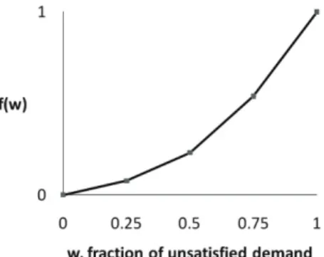
and serves demand quickly, but also incorporates equity by weighing units of demand differently. To incorporate equity, we consider a convex disutility function 𝑓(𝑤), where 𝑤 is the fraction of unsatisfied demand. Figure 2 plots an example function. Because the rate of change of the disutility is greater when the percentage of unsatisfied demand is closer to 1 (i.e., the demand served is low), the first pallets delivered receive greater benefit than the last.
Figure 2 An example piecewise-linear disutility function for unsatisfied demand
Similar to how the Z2 metric measures the demand-weighted arrival time, the Z3 metric minimizes the
disutility-weighted arrival time. The disutility function encourages a vehicle not to necessarily satisfy a node's entire demand
but rather to save supply to serve another node. Unlike Z2 where the change between delivered demand is accessible
from information in the model (𝑦𝑖𝑟), the change in disutility requires a calculation dependent on many variables. It is
easier to formulate the equivalent value of time-weighted disutility. We discretize time horizon into hours. For each hour 𝑡 ∈ 𝑻 = 1, ⋯ , 𝑇 and each node 𝑖 ∈ 𝑵, the percentage of unsatisfied demand of node 𝑖 at time 𝑡, 𝑤𝑖𝑡, is
calculated and a penalty equal to 𝑓(𝑤𝑖𝑡) is accrued. Thus, Z3, the time-weighted disutility is calculated as follows:
𝑤𝑖𝑡 = (1 − 𝑑𝑖1∑𝑟:𝑎𝑖𝑟<𝑡𝑦𝑖𝑟) (8)
𝑍3(𝑥, 𝑦) = ∑𝑇𝑡=1∑𝑁𝑖=1𝑓(𝑤𝑖𝑡) (9)
Equation (9) sums the penalties accrued due to the percentage of unsatisfied demands of each node 𝑖 ∈ 𝑵 over each hour 𝑡 ∈ 𝑻. In practice, 𝑓(𝑤𝑖𝑡) does not need to be calculated for every hour in 𝑻, but only when 𝑓(𝑤𝑖𝑡)
changes. This can be found by sorting the arrival times of deliveries to node 𝑖 and determining the time between successive deliveries. The following piecewise linear disutility function is used in our calculations:
𝑓(𝑤) = ⎩ ⎪ ⎨ ⎪ ⎧ 4𝑤13, 𝑤 < 0.25 �𝑤−1 13 , 0.25 ≤ 𝑤 < 0.5 16𝑤−5 13 , 0.5 ≤ 𝑤 < 0.75 24𝑤−11 13 , 𝑤 ≥ 0.75 (10)
The function is chosen to mimic the shape of a convex polynomial function. As more pallets are delivered, 𝑤 decreases; the progressively increasing slope ensures that the last pallets delivered are weighted less than the first.
3.3.4. An Illustrative Comparison of Objectives
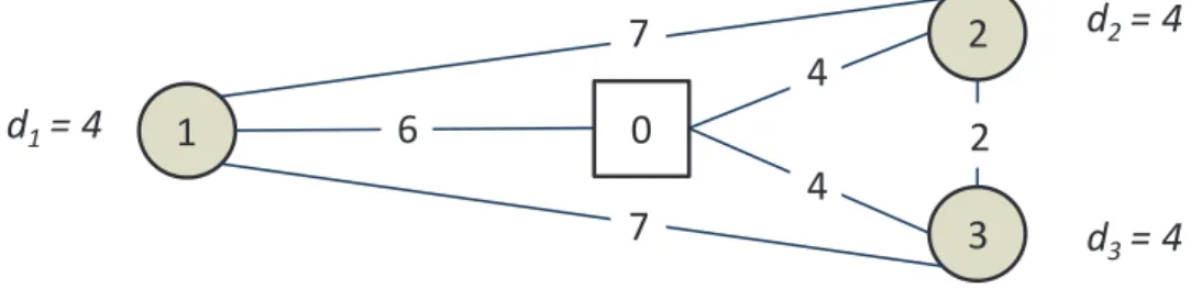
Figure 3 A sample distribution network with three recipient nodes. Arc lenghts are shown on each arc.
Consider an instance with two vehicles, each with capacity of 6 pallets. Figure 4 presents the optimal solutions for each LMDP variation. The figure shows the route path and delivery times and amounts at each node. Let 𝜋(𝑘) denote the route that is run by vehicle 𝑘. The routes obtained by the model variations differ in terms of delivery times and amounts. Table 1 displays the service level for each node (i.e., 𝑠𝑖 values) and the metric values for each
solution. Naturally, each solution optimizes its respective metric at the expense of other metrics.
Figure 4 Optimal solutions for the LMDP variations
3
2
4
4
1
6
7
7
d
1= 4
d
2= 4
d
3= 4
2
0
(a) Optimal solution for LMDP(Z1)
(b) Optimal solution for LMDP(Z2)
(c) Optimal solution for LMDP(Z3a) and LMDP(Z3b)
3 2 1 3 2 3 1 y1π(1)= 4, a1π(1)= 11 y2π(1)= 2, a2π(1)= 4 y2π(2)= 2, a2π(2)= 6 y3π(2)= 4, a3π(2)= 4 3 2 1 3 111 Vehicle 1 Vehicle 2 y2π(1)= 4, a2π(1)= 4 y3π(2)= 4, a3π(2)= 4 y1π(1)= 2, a1π(1)= 11 y1π(2)= 2, a1π(2)= 11 3 2 1 3 111 2 333 11 y2π(1)= 2, a2π(1)= 13 y2π(2)= 2, a2π(2)= 6 y3π(1)= 2, a3π(1)= 15 y3π(2)= 2, a3π(2)= 4 y1π(1)= 2, a1π(1)= 6 y1π(2)= 2, a1π(2)= 13
(d) Optimal solution for LMDP(Z3)
3 2 1 3 1 2 3333 y2π(1)= 1, a2π(1)= 13 y2π(2)= 3, a2π(2)= 6 y3π(1)= 1, a3π(1)= 15 y3π(2)= 3, a3π(2)= 4 y1π(1)= 4, a1π(1)= 6 0 0 0 0
Solution for Node service level Metric s1 s2 s3 Z1 Z2 Z3a Z3b Z3 LMDP(Z1) 11 5 4 27 80 7 3.09 19.46 LMDP(Z2) 11 4 4 34 76 7 3.30 19.00 LMDP(Z3a) 9.5 9.5 9.5 38 114 0 0 21.77 LMDP(Z3b) 9.5 9.5 9.5 38 114 0 0 21.77 LMDP(Z3) 6 7.75 6.75 29 82 1.75 0.72 17.38 Table 1 Performance of optimal solutions under different objectives
This simple example illustrates initial trends that guide our subsequent analysis. While all equity metrics have a common goal of reducing the disparity in service times among recipients, the model variations can yield differences in solutions. In the solution displayed in Figure 4(c), the two vehicles travel in opposite directions, each dropping off two units of demand at each of the nodes. The service level for all nodes is 9.5, yet nodes 1 and 3 can improve their service level without lowering the service level at node 2 if the vehicles that visit them first deliver their full demand. In such a solution, service levels of the nodes are 𝑠1= 6, 𝑠2= 9.5 and 𝑠3= 4. Thus in the LMDP(Z3a) and
LMDP(Z3b) solutions, nodes 1 and 3 are penalized to match the service level at node 2 to minimize the disparity
between service levels. While this is only one example, one can imagine in a large network, every route taking detours so that all nodes receive equally poor service. At a nominal cost to efficiency and efficacy (7% and 8% increase, respectively), the LMDP(Z3) solution greatly outperforms the LMDP(Z1) and LMDP(Z2) solutions with
respect to the Z3a and Z3b metrics. The large improvement in equity can be attributed to the allocation of demand at
node 3. Rather than completely serving node 3, vehicle 2 delivers an extra unit to node 2. The solution does not suffer large increases in Z1 and Z2 because there is still an incentive to serve demand quickly.
Additionally, this example illustrates how multiple optima to the LMDP models may produce unfavorable results. In the solution displayed in Figure 4(a), the solution can improve its Z2, Z3a, Z3b and Z3 without worsening its
Z1 metric value by reversing the route run by vehicle 1. In the computational studies, we utilize weighted secondary
objectives to select preferred options among multiple optima, as discussed in Section 3.5.1.
3.4. Analytical Properties
In this section, we explore route structures for the LMDP models. In an early SDVRP paper, Dror & Trudeau (1990) prove Property 3.1 regarding splitting in optimal SDVRP routes. We present the related Properties 3.2 and 3.3 for the LMDP(Z2) and LMDP(Z3). Property 3.4 validates our modeling assumption that each route is run at most
once. The proofs of Properties 3.2-3.4 are presented in Appendix A.
Property 3.1 (Dror and Trudeau): For LMDP(Z1), there exists an optimal solution where for every pair of nodes,
at most one vehicle visit both nodes.
Property 3.2: The result from Property 3.1 holds for LMDP(Z2).
Property 3.3: The result from Property 3.1 does not hold for LMDP(Z3).
Property 3.4: For each of the objective functions of the LMDP based on Z1, Z2 and Z3, there exists an optimal
solution where each route is run at most once.
Properties 3.1 and 3.2 imply that routes cannot share a subset of nodes with more than one recipient node. This suggests that for the LMDP(Z1) and LMDP(Z2), splitting is only beneficial for reasons linked to capacity. For the
LMDP(Z1), splitting of demand allows for fewer vehicles to be used. With the triangle inequality, a reduction in
routes run translates to a reduction in travel costs. In contrast, in the LMDP(Z2) where response time is minimized, it
is desirable to utilize the entire fleet of vehicles. Although the entire fleet is used, splitting may occur if a vehicle can reach a recipient earlier than the other vehicles but has insufficient supply to serve the recipient's full demand. Properties 3.1 and 3.2 can be used to add cuts to the formulation for their respective problems. The constraints ∑𝑟:�𝑏𝑖𝑟>0�&(𝑏𝑗𝑟>0)𝑥𝑟≤ 1 ∀ 𝑖,𝑗 ∈ 𝑁 may be added to the formulations of the LMDP(Z1) and LMDP(Z2). Because
splitting a node's demand among multiple vehicles can improve the equity-based Z3 objective, Property 3.1 does not
hold for LMDP(Z3), as shown in Figure 4(d). Splitting occurs so that a node may receive some of its initial supply
earlier at the expense of another node receiving its remaining supply later. We show how the differences between the properties regarding Z1 and Z2 with the property regarding Z3 impact route structure in the following section.
3.5. Computational Study of Small Instances
In this section, small instances of the LMDP models are solved using a commercial solver and solutions under the different objectives are compared. Section 3.5.1 introduces the test cases. Sections 3.5.2 and 3.5.3 present observations on route structure and performance metrics respectively.
3.5.1. Test Cases
Small instances are composed of an 8-node set and a 10-node set. For each set, five location distributions are paired with five demand distributions. The location distributions locate the nodes on a 100x100 square with the depot at the center; recipient nodes are either (1) clustered (C), (2) evenly distributed (E), or (3) randomly distributed (R1,R2,R3). The demand distributions allow demands to range between 1 to 4 pallets. Demand distributions are either (1) clustered by location creating low and high demand regions (C), (2) evenly distributed (E), or (3) randomly distributed (R1,R2,R3). Detailed descriptions of the instances are available in Appendix B of the expanded version of this paper (Huang, Smilowitz, & Balcik, 2010). Vehicles have a capacity of 10 pallets (𝐶=10); and the fleet size is one more than the minimum for feasibility (𝐾 = ⌈∑ 𝑑𝑖 𝑖⁄ ⌉ + 1). Travel costs are set to 𝐶
be the Euclidean distance between two nodes rounded to the nearest integer.
To choose preferred options among multiple optima, the following objectives are used: Z1 + αZ2 for LMDP(Z1),
Z2 + αZ1 for LMDP(Z2), and Z3 + αZ1 for LMDP(Z3), where α is chosen to be small enough to ensure that the
primary objective is minimized. The metric Z3 is not used as a secondary objective due its complexity and the
associated computational time. For the LMDP(Z3), Z1 is used as the secondary objective because efficacy (as
measured by Z2) is already partially addressed in the Z3 metric.
A C++ program using the C++ API of ILOG Concert Technology (ILOG, 2008) is developed; the mixed integer programs are solved using Concert 2.7 and CPLEX 11.2. The program is run on 2.4GHz 64-bit (4MB L2 cache) CPU machine with 8GB of RAM. To ensure computational tractability, we reduce the size of the candidate route set 𝑹, by restricting 𝑹 to only the feasible routes that do not visit more than 5 nodes. The restriction should not have a large impact on LMDP(Z2) and LMDP(Z3) solutions as the solutions aim to balance the demand roughly equally;
however, the restriction may affect LMDP(Z1) solutions where longer routes reduce the fleet's travel time.
Therefore, although these solutions are optimal for the given setting, we should note that the setting is restricted by route length. Lastly, a 60-hour limit is imposed on the solver for each LMDP instance.
3.5.2. Route Structure
Several observations can be made regarding the general nature of the optimal solutions for the different models of the LMDP. To illustrate these observations we provide a set of solutions for one 10-node instance of the LMDP variations in Figure 5. For each of the diagrams, with the exception of the depot at the center, the size of the node is representative of the amount of demand requested by the node.
Figure 5 Optimal solutions for Z1, Z2 and Z3 for a 10-node instance
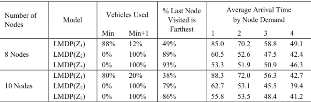
In Table 2, we present aggregate results for all instances. Columns 3 and 4 present the percentage of solutions which use the minimum number of vehicles and the percentage of solutions that use all available vehicles (one more than minimum, in this case). Column 5 displays the percentage of routes in which the last node visited coincides with the node on the route that is farthest from the depot. Columns 6 through 9 display the average arrival time of nodes for the different levels of node demand.
Number of
Nodes Model
Vehicles Used % Last Node Visited is
Farthest
Average Arrival Time by Node Demand Min Min+1 1 2 3 4 8 Nodes LMDP(Z1) 88% 12% 49% 85.0 70.2 58.8 49.1 LMDP(Z2) 0% 100% 89% 60.5 52.6 47.5 42.4 LMDP(Z3) 0% 100% 93% 53.3 51.9 50.9 46.3 10 Nodes LMDP(Z1) 80% 20% 38% 88.3 72.0 56.3 42.7 LMDP(Z2) 0% 100% 79% 62.7 53.1 45.5 39.4 LMDP(Z3) 0% 100% 86% 55.8 53.5 48.4 41.2
Table 2 Summary results for route structure across 8-node and 10-node instances Observation 1 Number of vehicles
With only a few exceptions, the optimal LMDP(Z1) solution uses the minimum number of vehicles (see columns
3 and 4 of Table 2). This point is made in Campbell et al. (2008); given the triangle inequality, minimizing travel costs results in the use of as few vehicles as possible. Instances where the LMDP(Z1) does not use the minimum
number of vehicles occur when multiple optima exist and the use of an extra vehicle can reduce service times without adding travel time. These exceptions occur in 12% of the 8-node instances and 20% of the 10-node instances. Optimal solutions to the LMDP(Z2) and LMDP(Z3) use all available vehicles which reduces the service
time of the nodes at the cost of increased travel time. In Figure 5(a), the LMDP(Z1) solution splits delivery to one
node with demand of four pallets to use a total of three vehicles instead of four. Observation 2 Route shape
Routes in optimal LMDP(Z1) solutions tend to be hooked-shaped, which is consistent with earlier studies of the
VRP (Daganzo, 2005). By curving back toward the depot, the routes reduce the distance from the final recipient back to the depot. In contrast, in the optimal solutions to the LMDP(Z2) and LMDP(Z3), where the line haul from the
final recipient back to the depot is not measured in the objective, optimal routes tend to be more ray-shaped, moving away from the depot (as seen in Figures 5(b) and (c)). We quantify these trends over all instances by measuring the percent of solutions in which the last node visited on a route is the farthest node from the depot on that route. For the 8-node instances, the last node visited is the farthest from the depot 49% of the time in the LMDP(Z1) solutions,
Demands 1 2 3 4
(a) LMDP(Z
1)
(b) LMDP(Z
2)
(c) LMDP(Z
3)
89% of the time in the LMDP(Z2) solutions, and 93% of the time in the LMDP(Z3) solutions. For the 10-node
instances, these percentages are 38%, 79%, and 86%, respectively. Observation 3 Impact of node demand
In the LMDP(Z2), where service time is measured in the objective, the routes are highly demand driven. Nodes
that have high demand are served at a premium, often at the expense of recipients with low demand. Nodes with demand 1 are often served last on their respective routes. In Figure 5(b), the LMDP(Z2) solution crosses two routes
so that a high-demand node may be served earlier. In the LMDP(Z3), as long as the nodes are visited by a single
vehicle, the nodes are served without regard to their demand level. Thus, the smallest nodes are treated more equally; they are served by the closest route and are not bypassed for nodes with higher demands. To quantify this observation we evaluate the average arrival time of nodes based on the demand of the node. This highlights two interesting trends. The LMDP(Z1) solution has longer arrival times for all nodes because LMDP(Z1) solutions use
fewer vehicles. The use of fewer vehicles means that the nodes on average receive their demand at later times. Further, nodes with lower demand often have longer arrival times as they are more likely to share their route with more nodes; again longer routes translate to longer arrival times. While each model exhibits a higher average arrival time for low-demand nodes, the deviation in arrival time is much lower in the LMDP(Z3) solutions than the other
models. Coincidentally, the hook-like characteristics of the routes in the LMDP(Z2) solution result from node
demand as the routes curve back to serve the smallest nodes that had been ignored earlier.
3.5.3. Metric Performance
Each model (LMDP(Z1), LMDP(Z2) and LMDP(Z3)) is evaluated relative to the five metrics (Z1, Z2, Z3a, Z3b and
Z3). To evaluate a solution with respect to metrics Z1, Z2, and Z3, we calculate the percentage difference between the
metric value of the solution and the metric value of the optimal solution for that metric. For example, let ZjLMDP(Zk)
be the Zj metric value of the optimal LMDP(Zk) solution and Zj* = ZjLMDP(Zj), then to evaluate the optimal LMDP(Z1)
solution with respect to Z2 we calculate Δ2LMDP(Z1)= (𝑍2�𝑀��(𝑍1)−𝑍2∗) 𝑍⁄ . For the metrics Z2∗ 3a and Z3b, the percent
difference is taken from the best solution among the LMDP(Z1), LMDP(Z2) and LMDP(Z3) solutions.
Table 3 summarizes the results of the 8-node and 10-node instances by aggregating the 25 instances with different demand and location distributions. Several observations may be made from Table 3.
Observation 4 The differences in route structure between the efficiency model (LMDP(Z1)) solutions and
solutions of the other variations translate into large differences in metric values.
By not considering travel from the last recipient to the depot, travel costs increase by 17% to 18%, on average, when Z1 is not the primary objective. The LMDP(Z2) and LMDP(Z3), by minimizing arrival times, implicitly reduce
distance, yet the LMDP(Z1) does not consider efficacy and equity, and these metrics are far from optimal when Z1 is
the primary objective, with average gaps of 29% for Z2, 65% to 72% for Z3a, and 64% to 68% for Z3b.
Model
Optimality Gap by Metric
8 Node Instances 10 Node Instances
Δ1 Δ2 Δ3 Δ3a Δ3b Δ1 Δ2 Δ3 Δ3a Δ3b LMDP(Z1) Avg - 29% 33% 65% 64% - 29% 34% 72% 68% Max - 65% 74% 135% 119% - 61% 68% 332% 222% Min - 7% 7% 0% 0% - 3% 2% 0% 0% LMDP(Z2) Avg 18% - 1% 2% 2% 17% - 2% 7% 4% Max 39% - 11% 15% 13% 39% - 14% 49% 30% Min 5% - 0% 0% 0% 2% - 0% 0% 0% LMDP(Z3) Avg 17% 2% - 0% 0% 17% 2% - 2% 1% Max 38% 33% - 5% 2% 39% 13% - 23% 18% Min 8% 0% - 0% 0% 1% 0% - 0% 0%
Table 3 Summary of deviation in metric values for LMDP models
Observation 5 The similarities in route structure of efficacy and equity (LMDP(Z2) and LMDP(Z3)) solutions
In contrast to the large difference observed between the LMDP(Z1) solutions and the other models, the optimal
LMDP(Z2) and LMDP(Z3) solutions have similar metric values; in many instances, the solutions are identical.
In terms of Z3a and Z3b, the LMDP(Z3) solutions perform slightly better than the LMDP(Z2) solutions. In the
8-node instances, the LMDP(Z2) averages 2% worse than the best solution while the LMDP(Z3) averages less than 1%
worse. In the results from the 10-node instances there is a larger gap. For Z3a and Z3b, the LMDP(Z2) is 7% and 4%
worse than the best solutions, respectively, while the LMDP(Z3) is only 2% and 1% worse. We conjecture that the
difference is due to a reduction in the amount of slack capacity that is available for the 10-node instances. This is supported by results with fewer vehicles as a reduction in number of vehicles results in a reduction of capacity.
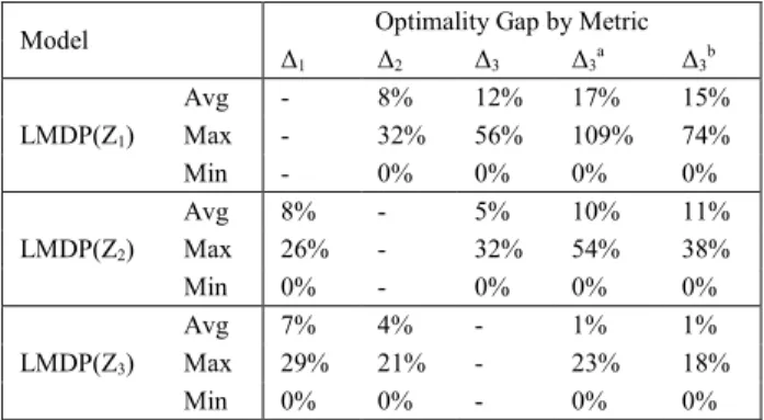
Table 4 presents results for the 8-node instances when the number of available vehicles is reduced to the necessary minimum. We could not obtain LMDP(Z3) solutions for many 10-node instances in the time limit.
Observation 6 When the three models are constrained to use the minimum number of vehicles, the differences in
metric values between the LMDP(Z1) solutions and the other two LMDP models decreases.
The loss of the extra vehicle results in closer metric values between the optimal solutions of the LMDP(Z1) and
the optimal solutions of the LMDP(Z2) and LMDP(Z3); in one instance, the solutions are identical for the three
models. We note the decrease in optimality gap when comparing Table 4 with Table 3. With respect to Z1, the
optimal LMDP(Z2) and LMDP(Z3) solutions average only 8% and 7% higher than the optimal LMDP(Z1) solutions,
respectively, and the LMDP(Z1) has Z2 and Z3 metric values averaging only 8% and 12% percent higher than the
optimal solutions for the LMDP(Z2) and LMDP(Z3), respectively.
Model Optimality Gap by Metric
Δ1 Δ2 Δ3 Δ3a Δ3b LMDP(Z1) Avg - 8% 12% 17% 15% Max - 32% 56% 109% 74% Min - 0% 0% 0% 0% LMDP(Z2) Avg 8% - 5% 10% 11% Max 26% - 32% 54% 38% Min 0% - 0% 0% 0% LMDP(Z3) Avg 7% 4% - 1% 1% Max 29% 21% - 23% 18% Min 0% 0% - 0% 0%
Table 4 Summary of deviation in metric values for LMDP models for 8-node instances with minimum number of vehicles
Reducing the number of vehicles effectively reduces capacity, and consistent with Observation 5, the differences between the LMDP(Z2) model and the LMDP(Z3) model become more prominent. With respect to Z2, the
LMDP(Z3) performs 4% worse and with respect to Z3, the LMDP(Z2) performs 5% worse. Most notable is that with
respect to the equity metric Z3b, the optimal LMDP(Z2) solutions average 10% worse than the best solution
compared to 1% of the optimal LMDP(Z3) solutions. We posit that as total demand approaches the total capacity of
the fleet, the percent difference in solutions becomes similar to the example in Section 3.3, where the LMDP(Z3)
exhibits a large improvement in equity at a nominal cost to efficiency and efficacy.
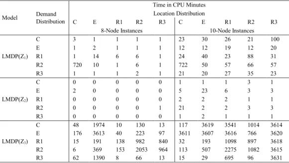
3.5.4. Computational Effort
Table 5 reports the time taken in CPU minutes. The LMDP(Z2) requires the least amount of time to solve. The
LMDP(Z3) requires the most time, occasionally reaching the 60-hour limit. For larger instances, heuristics are
Model Demand Distribution
Time in CPU Minutes Location Distribution
C E R1 R2 R3 C E R1 R2 R3
8-Node Instances 10-Node Instances
LMDP(Z1) C 3 1 1 1 1 23 30 26 21 100 E 1 2 1 1 1 12 12 19 12 20 R1 1 14 6 6 1 24 40 23 88 31 R2 720 10 1 6 1 722 50 57 66 57 R3 1 1 1 2 1 21 20 27 35 23 LMDP(Z2) C 0 0 0 0 0 1 1 1 3 1 E 2 0 0 0 0 5 23 6 3 3 R1 0 0 0 0 0 2 2 2 1 1 R2 0 0 0 0 1 21 2 2 3 3 R3 0 0 0 0 0 1 2 1 1 1 LMDP(Z3) C 48 1974 10 130 13 117 3619 3541 1014 3614 E 176 3613 40 223 97 3611 3607 3616 766 3620 R1 15 191 138 982 840 32 193 1098 897 3618 R2 6 369 153 2053 964 113 507 2275 1082 3615 R3 62 1390 8 66 13 15 29 695 96 3631
Table 5 Solution times in CPU minutes 4. Large Scale LMDP Instances
The previous section shows how route structure and metric values depend on the choice of objective function for the LMDP. Importantly, the results also show that the solution times for the LMDP(Z3) grow quickly. This section
proposes heuristics to solve larger instances of the LMDP. A greedy random adaptive search procedure (GRASP) framework is introduced in Section 4.1 to solve the LMDP(Z1) and LMDP(Z2). In Section 4.2, we present a new
approach for LMDP(Z3) since the methods used for the LMDP(Z1) and LMDP(Z2) cannot address the complexities
of this model. Section 4.3 presents a computational study of the large instances.
4.1. Heuristics for the LMDP(Z1) and LMDP(Z2)
To solve the LMDP(Z1) and LMDP(Z2), we utilize a GRASP framework (Feo & Resende, 1995). GRASP is a
metaheuristic in which a set number of repetitions is executed. Each repetition consists of a random constructive phase and a local improvement phase. In the constructive phase, a feasible solution is iteratively constructed. At each iteration, an insertion of a recipient into an existing route is selected randomly from a restricted candidate list of insertions which pass an evaluation function. The constructive phase is followed by an improvement phase where the constructive solution is improved via a deterministic local search to find a local optima. The best solution among all the repetitions is kept. Further details including a flowchart of the heuristic is provided in Huang et al. (2010).
4.2. Heuristic for the LMDP(Z3)
The heuristic for the LMDP(Z3) shares some similarities to the GRASP framework in that the heuristic employs a
set number of repetitions. Each repetition is evaluated with respect to Z3 and the best solution is kept. However, the
constructive and improvement methods of the LMDP(Z1) and LMDP(Z2) do not adapt well to the LMDP(Z3) due to
factors described in the following paragraph. Therefore, we pattern a heuristic for the LMDP(Z3) using an
alternative two-phase approach to incorporate the goals of equity, efficiency and efficacy. A detailed description of the heuristic (particularly the 2nd phase) is available in Huang et al. (2010).
In the LMDP(Z3), the dependency between routes prevents the decomposition of the problem by route; it is
difficult to determine the contribution towards the Z3 value from a single route. In addition, the value of Z3 is very
impact on the objective value. For these reasons, it is difficult to construct a solution or modify a solution to improve the objective as is done for the LMDP(Z1) and LMDP(Z2).
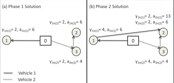
We draw on the insight that the optimal solution for the LMDP(Z3) delivers a portion of demand to each node
quickly and then distributes the remainder. The two-phase approach comprises of (1) an initial phase to deliver a fraction, β, of the demand to each node within a time τ and (2) a second phase to satisfy the remainder of the demand either by increasing the initial delivery amounts or by appending additional stops onto the routes. Note that the deliveries in the latter option are appended to the end of the routes rather than inserted into a route to ensure that the initial phase deliveries are performed before τ. Equity is incorporated by ensuring that each node receives a portion of its demand initially limiting the deviation in service level across nodes; efficacy and efficiency are incorporated via effective solutions for the two phases. The approach may be generalized to use node-specific βi
values to represent different urgency levels among the nodes.
The resulting solution is dependent on the parameter values of β and τ. A large β value and a small τ value correspond to serving most of the demand quickly; however, this is often infeasible. For a given β, if τ is too small, the instance is infeasible as it is not possible to serve β of the demand within τ. While one might expect that a large value of β would result in more equitable solutions, this is not always the case. A large value for β often requires a large value of τ to ensure feasibility. When τ is large, significant disparity in service levels may appear in the initial phase. A small value for β leaves opportunity for the service level to deviate in the second phase. Fortunately, as shown in Section 4.3.4, we find that the two-phase approach is fairly robust with respect to the choice of β.
In the initial phase, to ensure feasibility, the value of β is set a priori and the value of τ is set after the initial phase. To deliver the initial demand, we perform one repetition of the LMDP(Z2) heuristic on the graph 𝐺 = (𝑵0, 𝑨)
with reduced demands ⌈𝛽𝑑𝑖⌉ for all 𝑖 ∈ 𝑵. The solution to the LMDP(Z2) for the reduced demand problem produces
feasible routes that quickly deliver the initial demand; τ is set to be the latest arrival time in this solution. Using the example from Section 3.3.4, Figure 6(a) shows the solution after the initial phase when β=0.75. This solution yields a value of τ = 6.
The second phase is initialized with routes and deliveries from the initial phase; node 𝑖 begins with an unsatisfied demand equal to 𝑑𝑖− ⌈𝛽𝑑𝑖⌉. We refer to this demand as “unassigned demand” since these units are not associated
with routes at the start of the second phase. The heuristic designates each vehicle as capacity feasible or capacity infeasible based on a conservative estimate, which calculates the load on the vehicle plus the load from unassigned demand of nodes visited by the vehicle minus the vehicle capacity. A positive value represents a capacity infeasible vehicle and a negative value represents a capacity feasible vehicle. Delivery amounts are increased by 𝑑𝑖− ⌈𝛽𝑑𝑖⌉ for
all nodes on capacity feasible vehicles. For nodes visited by multiple vehicles, the heuristic increases the delivery amount to the node on the first vehicle found; for other vehicles, the delivery amount is not increased.
Figure 6 Solution using two-phase approach with β = 0.75
The heuristic then iteratively serves the unassigned demand. In each iteration, for each node with unassigned demand, the heuristic finds the cheapest way (in terms of travel time) to append the node to a capacity feasible vehicle. The cheapest option among all such nodes is executed. The feasibility status is updated for vehicles: if a vehicle becomes capacity feasible (i.e., the remaining nodes with unassigned demand on that route may be now served by the vehicle), the delivery amounts are increased to fully satisfy demand. The loop is repeated until all
demand is assigned. Like its LMDP(Z1) and LMDP(Z2) counterparts, the heuristic runs for 5000 iterations and the
best solution retained.
Figure 6(b) shows the final solution for the example using this approach. The route used by vehicle 1 is extended to deliver one pallet to nodes 2 and 3. The amount delivered to node 1 by vehicle 1 is increased to four pallets. The route used by vehicle 2 does not change. In this example, the solution is the optimal LMDP(Z3) solution.
4.3. Computational Study
In Section 4.3.1, we evaluate the ability of the heuristic to achieve high quality solutions for the small instances. For the large scale experiments, instances developed from the 100-node test cases from (Solomon, 1987) for VRP with Time Windows (VRPTW) (available at http://neo.lcc.uma.es/radi-aeb/WebVRP/) are used. In the original data set, there are four unique location configurations; instances differ by demands and time windows. Configurations C1 and C2 correspond to data sets with clustered locations; configuration R has random locations and configuration RC is a combination of random and clustered locations. For each C1 and C2 configuration, 10 instances are created by assigning nodes a random demand between 1 and 5; 20 instances are created for each R and RC configuration.
4.3.1. Performance against Optimal Restricted Solutions
We compare the heuristic solutions against the route-length restricted optimal solutions for the LMDP(Z1),
LMDP(Z2) and LMDP(Z3) for the 8-node and 10-node instances. Overall the heuristics perform very well. The
LMDP(Z1) heuristic matches or performs better than the solver solution in all but one instance with a gap of 3.8%.
Because the heuristics are not restricted to routes that visit at most 5 nodes, the LMDP(Z1) heuristic does on
occasion result in lower travel times than the solution found with CPLEX. The LMDP(Z2) heuristic finds optimal
solutions for every instance. The LMDP(Z3) heuristic achieves the optimal Z3 value in all but two of the 10-node
instances; in those cases, the gaps are 4.1% and 1.2%. Run times for the heuristics for the 8-node and 10-node instances for all models are less than a second of CPU time.
(a) Phase 1 Solution (b) Phase 2 Solution
3 2 1 3 1 2 3 Vehicle 1 Vehicle 2 y2π(2)= 2, a2π(2)= 6 y1π(1)= 2, a1π(1)= 6 y3π(2)= 2, a3π(2)= 4 y2π(1)= 2, a2π(1)= 13 y2π(2)= 2, a2π(2)= 6 y1π(1)= 4, a1π(1)= 6 y3π(2)= 4, a3π(2)= 4 (1)= 4, a1π(1)= 6 3 2 1 3 1 2 3
0
0
4.3.2. Metric Performance for Large Instances
Since there is no guarantee of optimality in the heuristic solutions, in the large instances, we evaluate the solutions with respect to each metric by calculating the percent difference between the metric value for that solution from the best solution for that metric among the three heuristic solutions. Table 6 aggregates the 60 large instances and presents the percent difference between each heuristic and the best solution among the heuristics. Results for each location configuration is provided in Huang et al. (2010), but the three location types do not exhibit a large difference; hence, results presented here are aggregated over the 60 instances.
Heuristic for Gap by Metric Δ1 Δ2 Δ3 Δ3a Δ3b LMDP(Z1) Avg 0% 27% 31% 63% 37% Max 0% 41% 43% 115% 63% Min 0% 15% 14% 6% 9% LMDP(Z2) Avg 16% 1% 4% 8% 4% Max 26% 3% 9% 50% 21% Min 9% 0% 1% 0% 0% LMDP(Z3) Avg 16% 1% 0% 1% 0% Max 26% 11% 0% 18% 5% Min 6% 0% 0% 0% 0%
Table 6 Summary of deviation in metric values for LMDP heuristics for large instances
While it is intuitive that each heuristic solution should perform its best on the model it attempts to solve, the LMDP(Z3) heuristic solution often outperforms the LMDP(Z2) heuristic solution with respect to Z2. The trends in
relative metric values are similar to the observations seen in Section 3.5.3 in that the metric values for the solutions for the LMDP(Z2) model and LMDP(Z3) model are similar to each other and differ more greatly with the solutions
for the LMDP(Z1); furthermore, while the LMDP(Z2) and LMDP(Z3) exhibit similar solutions, the LMDP(Z3) in
general yields solutions that are more equitable.
Averaging over all the instances, for the Z2 and Z3 metrics, the LMDP(Z1) solutions average 27% and 31%
respectively higher than the best heuristic solution for the respective metrics. With regards to the Z1 metric, the
heuristic LMDP(Z2) and LMDP(Z3) solutions both average 16% higher than the best heuristic Z1 solutions attained
by the LMDP(Z1) heuristic. With respect to the equity metric Z3b, the optimal LMDP(Z2) solutions are on average
4% higher than the best heuristic solution while the LMDP(Z3) solutions are on average less than 1% higher.
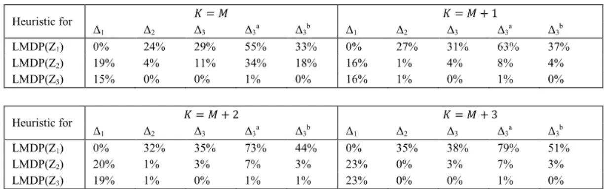
To examine the effect of excess capacity, we alter the number of vehicles and study its effect. Let 𝑀 denote the minimum number of vehicles necessary for feasibility (𝑀 = �1
𝐶∑ 𝑑𝑖 𝑖�). Table 7 presents the percentage differences
with 𝑀, 𝑀 + 1, 𝑀 + 2, and 𝑀 + 3 vehicles.
Heuristic for 𝐾 = 𝑀 𝐾 = 𝑀 + 1 Δ1 Δ2 Δ3 Δ3a Δ3b Δ1 Δ2 Δ3 Δ3a Δ3b LMDP(Z1) 0% 24% 29% 55% 33% 0% 27% 31% 63% 37% LMDP(Z2) 19% 4% 11% 34% 18% 16% 1% 4% 8% 4% LMDP(Z3) 15% 0% 0% 1% 0% 16% 1% 0% 1% 0% Heuristic for Δ 𝐾 = 𝑀 + 2 𝐾 = 𝑀 + 3 1 Δ2 Δ3 Δ3a Δ3b Δ1 Δ2 Δ3 Δ3a Δ3b LMDP(Z1) 0% 32% 35% 73% 44% 0% 35% 38% 79% 51% LMDP(Z2) 20% 1% 3% 7% 3% 23% 0% 3% 7% 3% LMDP(Z3) 19% 1% 0% 1% 1% 23% 0% 0% 1% 0%
Table 7 Average deviation in metric values for LMDP model heuristics solutions with different numbers of vehicles
As the number of available vehicles increases, the percent difference between the heuristic LMDP(Z1) solution
of vehicles in the LMDP(Z1), while the opposite is true for the LMDP(Z2) and LMDP(Z3). We also note that as more
vehicles become available, the LMDP(Z2) and LMDP(Z3) metric values become closer; the extra capacity of the
vehicles allows for greater parallel delivery reducing the impact of node demand.
4.3.3. Route Structure for Large Instances
Unlike the small instances investigated in Section 3.5, the solutions in the large instances exhibit demand splitting among multiple vehicles. The choice of model also influences the degree to which visits to a node are split
among multiple vehicles. For instance, the LMDP(Z3) solution should have a higher number of nodes visited by
multiple vehicles due to splitting for both capacity and equity reasons.
Heuristic For
Average number of nodes visited by: 1 vehicle 2 vehicles 3+ vehicles LMDP(Z1) 93.38 6.60 0.02
LMDP(Z2) 90.65 8.87 0.48
LMDP(Z3) 89.52 9.73 0.75
Table 8 Average number of split deliveries in 100-node instances
Table 8 shows the number of vehicles visiting each node for each of the heuristic solutions to the LMDP(Z1),
LMDP(Z2) and LMDP(Z3). As expected, the heuristic for the LMDP(Z3) exhibits more splitting than the other two
models albeit by a slim margin. Further, the splitting is not excessive as the large majority of the nodes are served by only one vehicle. The emergence of splitting in the solutions impacts route structure; because the LMDP(Z3)
heuristic attempts to deliver to each node a fraction of its demand, some routes must double back to deliver to nodes whose demand can not be satisfied before time τ. As a result, the ray-like structure seen in the routes of the LMDP(Z3) for small problems is no longer seen in the larger cases.
4.3.4. Choice of β for LMDP(Z3) Heuristic
This section investigates how the value of β, the fraction of demand that is served in the initial phase of the LMDP(Z3) heuristic, impacts the LMDP(Z3) solutions. Specifically, we examine how the choice of β affects the
degree of splitting and metric values of the LMDP(Z3) solutions.
Figure 7 shows the effect of β on splitting. The curve shows the percentage of nodes that are visited by multiple vehicles in the LMDP(Z3) solutions with respect to β aggregated across the 60 large instances. The discrete nature of
the curve is due to the ceiling function when delivering ⌈𝛽𝑑𝑖⌉.
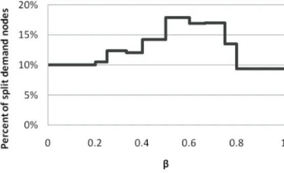
Figure 7 Percentage of split-demand nodes relative to β
Splitting is minimal when β is close to 0 or close to 1. When β=0, the LMDP(Z3) heuristic reduces to its second
phase in which splitting for equity does not occur. At this point 10% of the nodes are visited by multiple vehicles due to vehicle capacity. As β increases, the number of split nodes increases peaking at 18% in the interval between β=0.5 and β=0.6. As β increases further, the amount of nodes split drops off rapidly. When β=1, the LMDP(Z3)
heuristic reduces to the initial phase of the heuristic and thus is equivalent to the LMDP(Z2) heuristic; therefore no
splitting is done for equity reasons.
Figure 8 Percent change of heuristic LMDP(Z3) metric values from base case relative to β
Figure 8 shows how the metric values of the LMDP(Z3) change as β changes. For each metric, we plot the
percent difference in metric value with respect to β compared to the metric value when β=0.25, averaged over all 60 instances.
Overall, the choice of β does not have a large impact on the metric values of solutions. With the exception of the Z3a metric, the values do not change by more than 5%. However, small trends are observed. The Z1 and Z2 metric
values increase (decrease) with increases (decreases) in node splitting observed in Figure 7. As more nodes are visited by multiple vehicles to improve equity, the distance traveled and total wait times increase. Conversely, the metric values for the equity metrics Z3a, Z3b and Z3 improve when β takes values that encourage more splitting.
Combining these results and factoring the rate of change in the curves in Figure 8, a small value for β achieves good improvements in efficiency and efficacy, with a modest loss of equity.
One can set β considering the tradeoffs among metrics and characteristics of the relief setting. For instance, if efficiency and efficacy are emphasized, Figure 8 suggests a low value of β is preferable; if equity is more of a concern, a higher value of β may be more appropriate.
5. Concluding Remarks
This paper formulates efficacy and equity metrics and shows that there is a significant difference between solutions that focus on both efficacy and equity and solutions that focus on the traditional commercial concern of efficiency. In the following sections, we discuss the implication of our findings.
5.1. Practical Implications
The results from this paper provide several insights for relief operations. In practice, relief organizations tend to utilize a vehicle fleet consisting of many small vehicles, unlike in commercial settings where large vehicles are available and may be preferable to achieve economies of scale. The organizations acquire transportation resources locally as maintaining and shipping large vehicles long distances, especially overseas, can be very expensive and time consuming. Further, local drivers are more knowledgeable of the regions’ geography and customs. Characteristics of the post-disaster transportation network affect vehicle selection decisions; for instance, remote locations in a rural area may only be accessed by small trucks. Observation 1 suggests that operating a large number of small vehicles has the additional benefit of resulting in more effective and equitable aid distribution at the expense of a modest increase to traveling and operating costs (e.g., costs of fuel, drivers, etc.).
While having a large fleet of small vehicles is beneficial in improving the efficacy and equity of relief deliveries, operating and coordinating a large fleet might be difficult for relief logisticians in the field. For instance, the logistics coordinator of the Finnish Red Cross was responsible for coordinating a fleet of 150 trucks from a single warehouse during the relief operations after the Pakistan earthquake in 2005 (Mantyvaara, personal communication, 2010). While there is an increasing effort to develop and improve the logistics software in the relief sector, the current software is mostly used for tracking, monitoring and reporting purposes and lacks modules that would support operational decisions. Indeed, routing and delivery scheduling decisions are made mostly according to the insights and experiences of the logisticians. Our heuristics described in Section 4 are efficient and easy to understand, and hence could be a valuable decision support tool to manage large scale last mile operations, if embedded in such software. Observations 2 and 3 focusing on route shape dependent on objective and node demand represent a first step to developing even simpler rules-of-thumb so that a coordinator may make decisions without advanced computing resources.
In humanitarian relief environments, there may be large differences between the needs of populations at different locations. Although Formulation (1) does not explicitly differentiate populations in terms of their vulnerabilities, our heuristic approach can easily incorporate the criticality and urgency of the needs at different locations. Specifically, relief supply deliveries can be prioritized by modifying βi and τ values so that vehicles can reach more vulnerable
locations first.
While setting the β values, it is also important to evaluate the characteristics of the relief network. As discussed earlier, while splitting may help achieve more equitable and effective solutions, it also increases travel costs. Moreover, in regions where the transportation network is damaged and security is a concern, or when access to certain locations is problematic for other reasons such as poor weather conditions, relief organizations may prefer satisfying the demand of a location in a single delivery if possible. In such cases, a small β value leading to few splits may be more reasonable.
5.2. Future Work
One avenue of extension to this work is to analyze the LMDP variations under uncertainty, both in relaxing demands and travel times. In the chaotic environment that follows the immediate aftermath of a disaster there is significant uncertainty. For instance, demand is not immediately known and can only be roughly estimated. Also, travel times between two locations can be uncertain due to damaged infrastructure and unreliable information regarding the road conditions. Therefore, insights into the behavior of efficiency, efficacy, and equity under a stochastic setting would be valuable.
Another avenue of focus is to use the insights gained to generate rule-of-thumb solutions that are easy to find and simple to implement. Because relief agencies often lack technology and computational resources, solutions which may be implemented by hand would be valuable. Rule of thumb solutions would also be quick to calculate and in
planning stages could serve as an approximation for costs until more sophisticated solutions are found. Our analysis of stylized distribution problems is an important first step in this area.
To gather insight on how to address concerns of efficiency, efficacy and equity, the LMDP has been separated into three variations. However, in practice, agencies must handle these concerns concurrently. Therefore, it may be important to consider a multi-objective variation of the LMDP which combines the three factors into a single objective.
Acknowledgements
This research has been supported by the National Science Foundation, CMMI 0348622 and CMMI 0654398, as well as the Northwestern University Transportation Center. We also would like to thank the many relief organizations that provided insights for the paper, including Ari Mantyvaara.
References
Archetti, C., Savelsbergh, M., & Speranza, M. (2006). Worst-case analysis for split delivery vehicle routing problems. Transportation Science , 40 (2), 226-234.
Archetti, C., Savelsbergh, M., & Speranza, M. (2008). To split or not to split: that is the question. Transportation Research Part E , 44, 114-123. Balcik, B., Beamon, B., & Smilowitz, K. (2008). Last mile distribution in humanitarian relief. Journal of Intelligent Transportation Systems , 12
(2), 51-63.
Balcik, B., Iravani, S., & Smilowitz, K. (2011). A Review of Equity in Nonprofit and Public Sector: A Vehicle Routing Perspective. Encyclopedia of Operations Research and Management Science .
Barbarosoglu, G., & Arda, Y. (2004). A two-stage stochastic programming framework for transportation planning in disaster response. Journal of the Operational Research Society , 55 (1), 43-53.
Barbarosoglu, G., Ozdamar, L., & Cevik, A. (2002). An interactive approach for hierarchical analysis of helicopter. European Journal of Operational Research , 140 (1), 118-133.
Beamon, B., & Balcik, B. (2008). Performance measurement in humanitarian relief chains. International Journal of Public Sector Management , 21 (1), 4-25.
Campbell, A., Vandenbussche, D., & Hermann, W. (2008). Routing for relief efforts. Transportation Science , 42 (2), 127-145. Daganzo, C. (2005). Logistics Systems Analysis. Berlin: Springer.
Dror, M., & Trudeau, G. (1989). Savings by split delivery routing. Transportation Science , 23, 141-145. Dror, M., & Trudeau, G. (1990). Split Delivery Routing. Naval Research Logistics , 37, 383-402. Erkut, E. (1993). Inequality measures for location problems. Location Science , 1 (3), 199-217.
Feo, T., & Resende, M. (1995). Greedy randomized adaptive search procedures. Journal of Global Optimization , 6, 109-133.
Haghani, A., & Oh, S. (1996). Formulation and solution of a multi-commodity, multi-modal network flow model for disaster relief operations. Transportation Research Part A , 30 (3), 231-250.
Huang, M., Smilowitz, K., Balcik, B. (2010) Models for Relief Routing: Equity, Efficiency and Efficacy (Expanded Version) available at http://www.iems.northwestern.edu/docs/working_papers/michael_huang_dec10.pdf
ILOG. (2008). ILOG CPLEX 11.2 User's Manual.
Knott, R. (1987). The logistics of bulk relief supplies. Disasters , 11 (2), 113-115.
Knott, R. (1988). Vehicle scheduling for emergency relief management: A knowledge-based approach. Disasters , 12 (4), 285-293.
Lin, Y.-H., Batta, R., Rogerson, P., Blatt, A., & Flanigan, M. (2009). A logistics model for delivery of prioritized items: Application to a disaster relief effort. Department of Industrial and Systems Engineering, University at Buffalo (SUNY), Buffalo .
Marsh, M., & Schilling, D. (1994). Equity measurement in facility location analysis: A review and framework. European Journal of Operational Research , 74 (1), 1-17.
Mulligan, G. (1991). Equality measures and facility location. Papers in Regional Science , 70 (4), 345-365.
Ozdamar, L., Ekinci, E., & Kucukyazici, B. (2004). Emergency logistics planning in natural disasters. Annals of Operations Research , 129, 217-245.
Russell, T. (2005, June). The humanitarian relief supply chain: Analysis of the 2004 South East Asia earthquake and tsunami. Massachusetts Institute of Technology.
Shen, Z., Dessouky, M., & Ordonez, F. (2009). A two-stage vehicle routing model for large-scale bioterrorism emergencies. Networks , 54, 255-269.
Solomon, M. (1987). Algorithms for the vehicle routing and scheduling problem with time windows. Operations Research , 35, 254-265. Tzeng, G., Cheng, H., & Huang, T. (2007). Multi-objective optimal planning for designing relief delivery systems. Transportation Research Part
E , 43 (6), 673-686.
Van Hentenryck, P., Bent, R., & Coffrin, C. (2010). Strategic planning for disaster recovery with stochastic last mile distribution. In A. Lodi, M. Milano, & P. Toth, Integration of AI and OR Techniques in Constraint Programming for Combinatorial Optimization Problems (Vol. 6140, pp. 318-333). Springer Berlin / Heidelberg.
Van Wassenhove, L. (2006). Blackett Memorial Lecture Humanitarian Aid Logistics: Supply chain management in high gear. Journal of the Operational Research Society , 57, 475-489.
Yi, W., & Ozdamar, L. (2007). A dynamic logistics coordination model for evacuation and support in disaster response activities. European Journal of Operational Research , 179, 1177-1193.