SIMPLE AND ACCURATE CELL MACROMODELS FOR THE SIMULATIONS OF CELLULAR NEURAL NETWORKS

(1)

ISTANBUL UNIVERSITY ENGINEERING FACULTY JOURNAL OF ELECTRICAL & ELECTRONICS

YEAR VOLUME NUMBER : 2002 : 2 : 1 (423-436)

SIMPLE AND ACCURATE CELL MACROMODELS FOR THE

SIMULATIONS OF CELLULAR NEURAL NETWORKS

1

Baran TANDER

2

Mahmut UN

1

Kadir Has University, Vocationary School, 34590 Bahçelievler Istanbul, TURKEY

2

Istanbul University, School of Engineering Department of Electrical and Electronics Engineering 34850 Avcilar Istanbul, TURKEY

1_e-mail: _{[email protected]} 2_e-mail: _{[email protected]}

ABSTRACT

In this paper, two simple and accurate cell macromodels for PSPICE simulations of Cellular Neural Networks (CNNs) are designed. Firstly, a brief information about CNNs and their benefits are introduced. Then the nonlinear differential equations that characterize the CNNs a nd the equivalent cell circuit given by Chua and Yang which realizes these equations are presented. With appropriate source transformations, another cell equivalent that employs voltage controlled-voltage sources instead of voltage controlled-current sources is developed. By substituting the dependent sources with their actual circuits for both equivalents, complete systems which are suitable for PSPICE macromodeling are derived. Responses of astable and stable CNNs are analyzed with the proposed macromodels and satisfactory results are observed after the simulations. The benefits and drawbacks of the macromodels are also discussed in the conclusion section.

Keywords: Cellular Neural Networks, Equivalent Circuits, Simulation, PSPICE, Macromodels.

ÖZET

Bu makalede, Hücresel Sinir Aðlarýnýn PSPICE benzetimleri için basit ve güvenilir iki hücre makromodeli tasarlanmýþtýr. Ýlk olarak, kýsaca Hücresel Sinir Aðlarý ve avantajlarýndan bahsedilmiþtir. Ardýndan, Hücresel Sinir Aðlarýný karakterize eden nonlineer d iferansiyel denklem takýmlarý tanýtýlmýþ ve bu denklemleri gerçekleyen, Chua ve Yang tarafýndan tasarlanmýþ eþdeðer devreler sunulmuþtur. Uygun kaynak dönüþümleri yapýlarak, gerilim kontrollu akým kaynaklarý yerine gerilim kontrollu gerilim kaynaklarý kullanan yeni bir eþdeðer devre türetilmiþtir. Her iki eþdeðerdeki baðýmlý kaynaklar gerçek devreleriyle deðiþtirilerek PSPICE makromodellemesine uygun tam yapýlar elde edilmiþtir. Önerilen makromodellerle kararlý ve kararsýz Hücresel Sinir Aðlarýnýn benzetiml eri yapýlmýþ ve tatmin edici sonuçlar gözlenmiþtir. Makromodellerin avantaj ve dezavantajlarý sonuçlar kýsmýnda tartýþýlmýþtýr.

(2)

424

1 Introduction: CNNs

CNNs are a class of dynamical neural networks and were first proposed by Chua and Yang in 1988 [1]. In the CNN architecture, the cells (neurons) are connected to each other with a neighborhood definition given in (1).

{

}

{

Ckl k i l j r k M l N

}

j i Nr = − − ≤ ≤ ≤ ≤ ≤ ∆ 1 , 1 , , max ) , ( ) , ( (1) In the above formula, r is the neighborhood dimension and (i, j), (k, l) are the locations of the cells in an MxN-cell network. Because of their two dimensional structure, CNNs are very suitable for image processing applications [2] as well as for some optimization problems and their implementation is easier when compared with the Hopfield Dynamical Neural Networks since a cell can only interact with its nearest neighbors for an

r

=

1

neighborhood dimension here, and it is clear that this reduces the numb er of connections (therefore the number of weight coefficients) between the cells in the whole system. Moreover, only two 3x3 weight coefficient matrices and a constant threshold value will be enough to represent a CNN having a neighborhood dimension of one. A portion of the structure mentioned above is shown in figure – 1.

The state equation of the C(i, j) cell can be written as:

0 =

⋅

−

⋅

−

+

−

∑

∈ ∈ ) j , i ( N ) l, k ( C l, k ) j , i ( N ) l, k ( C l, k j , i j , i j , i r r

u

)

l,

k

;

j

,

i

(

B

y

)

l,

k

;

j

,

i

(

A

x

I

& (2a) where,

[

1

1 ]

2

1 )

(

_, _, _, ,l

=

kl

=

kl

+

−

kl

−

k

f

x

y

(2b) is a piecewise linear function.

If we consider an MxN-cell structure and write the above equations in matrix form, we will have:

I

U

B

X

A

X

&

=

−

+

*

f

(

)

+

*

+

(3)

Where xi,j is the “state” of the cell C(i, j); yk,l is the “output” of C(k, l); uk,l is the “input” of C(k,

l); A(i, j; k, l) is the “weight coefficient” between C(i, j) and the yk,l; B(i, j; k, l) is another “weight

coefficient” between C(i, j) and the uk,l; and finally, Ii,j is a “threshold” value common for all cells. The weight coefficient matrices A and B are also called “Cloning Template” and “Control Template” respectively. The constant value of xi,j when

t

→

∞

is called “

x

_i∞,_j stable equilibrium

point”. Design of a CNN is the computation of

A, B matrices and I scalar. “ * ” is the

two-dimensional convolution operator. The block diagram of a CNN cell is shown in figure – 2 [3].

2 Circuit Equivalents of CNNs

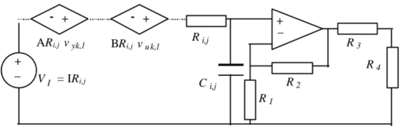
We can also represent a CNN cell by means of a dynamical circuit having conventional components like the one in figure – 3. This cell equivalent given by Chua and Yang in [1], employs linear resistors, capacitors, dependent and independent current/voltage sources and a nonlinear dependent voltage source. Note that, (2a) is the node equation of the state vxi,j.

The nonlinear voltage controlled-voltage source at the output can be designed with a simple opamp circuitry sketched in figure – 4(a) [4]. Since the opamps are not ideal, the maximum output voltages will be equal to

(

V

cc

−

2 )

not

Vcc, therefore the conditions,

R

₁

=

R

₄,

3 2

R

=

and

1 (

2 )

1 2

≅

−









+

V

cc

R

will give the piecewise linear activation function characteristic defined with (2b).

There are many articles in the literature about the circuit designs of CNNs [5], [6], however they all propose the dependent current sources for the addition unit at the input of the cell. By performing appropriate source transformations, the “state” node can be converted to a mesh that includes voltage controlled-voltage sources [7] as shown in figure – 5. In this topology, we will only deal with the voltages and also it will enable us to use the basic opamp adder circuit for serial connected dependent sources.

3 Macromodel Design

Macromodels are circuit blocks used for modeling the ICs in PSPICE [8]. This simplifies the simulation procedure because it reduces the number of components and nodes in the models. The analytical solutions of the differential equations that represent the CNN structures are

(3)

425 quite time consuming. Therefore, numerical

methods and simulation tools like PSPICE plays a crucial role in the analysis of such systems.

3.1. HSA10 Macromodel

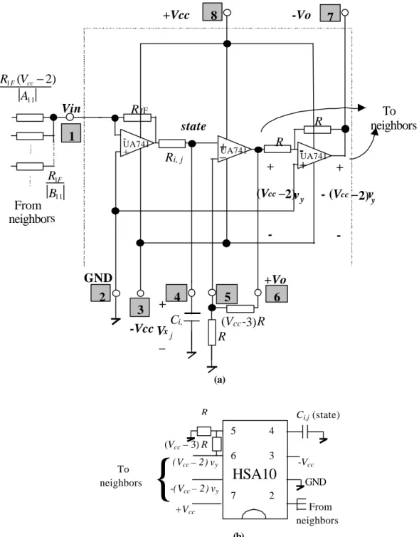
We first used the complete circuit shown in fig. – 6(a) for our macromodel design and named it HSA10. Indeed, it is a cascaded adder, non-inverting and non-inverting opamp blocks that uses the UA741 macromodel. It can be considered as an 8-pin analog IC. A cell circuit constructed by HSA10 is given in figure – 6(b).

In this circuit, the output voltage of a cell will be

(

−

2 )

±

V

cc volts instead of

±

1 V

in the stable case since the noninverting amplifier block has a maximum gain of

(

V

_cc

−

2 )

. The resistances that represent the weight coefficients between the inputs and the states can be calculated by dividing the

R

_F₁feedback resistance in the adder circuit to the absolute value of the matching element at the control template B; and the resistances that determine the weight coefficients between the outputs and states can be found by dividing the

R

_F₁

⋅

(

V

_cc

−

2 )

to the absolute value of the matching element in the cloning template A. Both +y (+vo) and –y (-vo) outputs are available for positive and negative values of the elements in the template matrices.

3.2. HSA11 Macromodel

Another macromodel is HSA11, which uses the cell circuit given in [9] derived from the Chua and Yang’ s conventional equivalent. In this topology, a voltage controlled current source and two inverting amplifier blocks built with UA741 macromodel are cascaded as shown in figure – 7(a). The operation of the circuit is approximately the same with HSA10. Here, the only difference is that the currents from the neighbor cells are added at the input stage. The complete cell circuit with HSA11 is sketched in figure – 7(b).

4 Simulations

In this section, three CNN structures with different dimensions and templates are simulated in order to test the validity of our macromodels. The results are verified with the ones that were found by Chua and Yang’ s equivalent in [1].

4.1 1x2-Cell Oscillating CNN

Simulation

Firstly, a 1x2-cell CNN with opposite-sign template [10] is analyzed with the macromodels. The differential equations that represent such a CNN are given below:

2 1 1 1 x y y x

v

&

=

−

+

α

⋅

−

β

⋅

(4a) 2 1 2 2 x y y x

v

&

=

−

+

β

⋅

+

α

⋅

(4b)

If we write these equations in a matrix form,













=

























⋅













−

+













⋅













−

=













20 10 2 1 2 1 2 1 2 1 0 0 ; 1 0 0 1 X X ) ( x ) ( x ) x ( f ) x ( f x x x x

α

β

α

& & (5) will be found. Where the f(.) is the activation function with piecewise linear characteristic. The structure that realizes the above equations is sketched in figure – 8.

For specific

α

and

β

values it was shown that this system will oscillate. We need two macromodels for the simulation of this CNN. The

α

and

β

values are chosen as 2 and 5 respectively. These correspond to 6500Ω and 2600Ω resistances for the weight coefficient resistors if

±

V

_cc

=

±

15 V

and

R

_F₁

=

1

kΩ since ij cc F j i

a

V

R

1

(

2 )

,

−

⋅

=

. The

v

_x

(

0 )

initial conditions for the voltages of the capacitors at each cell are 0.1V. A comparison between Chua and Yang’ s equivalent and our macromodel for the

v

_x₁

(

t

)

and

v

_x₂

(

t

)

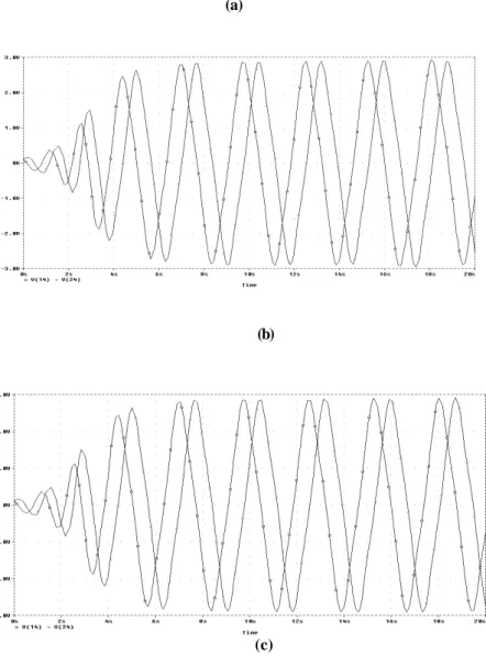
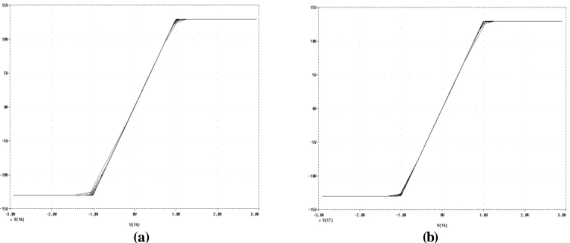
state voltages is shown in figure – 9.

The piecewise linear voltage characteristic between vx and vy in a cell can also be observed from the simulations as shown in figure – 10.

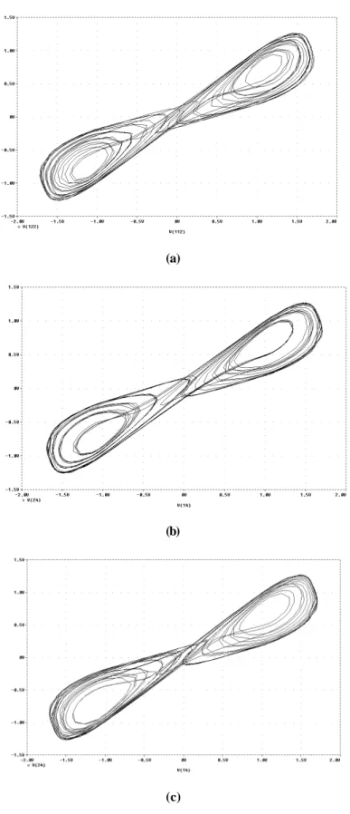
4.2. 1x3-Cell Chaotic CNN Simulation

It is possible to generate chaotic signals by using CNNs. Here, we simulated a 1x3-cell chaotic CNN with the proposed macromodels. The differential equations that represents such a system are given by Zou and Nossek in [9]. If we rewrite the mentioned equations in matrix form, we will have:

(4)

426           ⋅           − − − − − +           ⋅           − =           3 2 1 3 2 1 3 2 1 1 4 4 2 3 4 4 1 1 2 3 2 3 2 3 25 1 1 0 0 0 1 0 0 0 1 y y y . . . . . . . . x x x x x x & & & ;













=













1 .

0

1 .

0

1 .

0 )

0 (

)

0 (

)

0 (

3 2 1

x

The block diagram representation of the above form is shown in figure – 11.

The phase planes for the vx state voltages of C(1,1) and C(1,2) cells are plotted in figure – 12. In this case, the weight coefficient resistance matrix between the cells for our macromodels will be equal to:

Ω             ≅ ⋅ Ω ≅ = k . . . . . V k R . . . RA Ai,j 13 5 2954 5 4062 5 2954 2 11818 1 1 13 1 5 4062 5 4062 5 4062 10400

It is obvious that the orbits will not be the same in the three circuits since the chaotic systems are extremely sensitive to the initial conditions, circuit parameters and voltage characteristics; therefore to the circuit topology and rounding errors in PSPICE program. However the double scrolls observed from the simulations prove that our macromodels can generate chaotic signals.

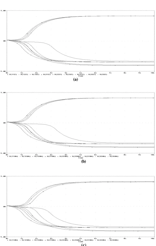
4.2 3x3-Cell Stable CNN Simulation

As the last example, we simulated a 3x3-cell stable CNN with the following templates A and

B and with a threshold value of I which are used

in a feature extraction application in an image processing problem [4]. Note that, in the previous sections, neither we used the two -dimensional convolution, nor the input and threshold values were included in the equations. In the following application the two-dimensional convolution operator will be employed and also the U and I will be used. Below is the matrix form of the mentioned system: I U X X X B A +           − − − − − − − − − +           − − − − − − − − + − = * . . . . . . . . . ) ( f * . . . . . . . . . 4 4 4 4 4 4 3 4 4 4 4 4 4 2 1 4 4 4 4 4 4 3 4 4 4 4 4 4 2 1 & 1433 0 1396 0 1439 0 1396 0 0698 0 1396 0 1439 0 1396 0 1433 0 1836 0 2724 0 1764 0 2523 0 7405 3 2523 0 1764 0 2724 0 1836 0 I=0.2540

The U input is a 3x3-pixel portion of the image that was processed and set equal to the initial condition X(0): U=X(0)













=

1008

.

0 1176

.

0 1345

.

0 1092

.

0 1261

.

0 1429

.

0 1261

.

0 1429

.

0 1513

.

0

The weight coefficient resistors realizing the above templates when

±

V

_cc

=

±

15 V

and

1

=

F

R

kΩ, are: Ω             ≅ ⋅ Ω ≅ = 70806 47724 73696 51526 5 3475 7405 3 13 1 51526 73696 47724 70806 . . V k R RA Ai,j Ω             ≅ − Ω ≅ = 4 6978 3 7163 3 6949 3 7163 6 14326 0698 0 1 3 7163 3 6949 3 7163 4 6978 . . . . . . k R . . . . RB Bi,j

Ω

=

∴

=

V

R

k

V

_I

0 .

254

_I

1

The

v

∞_x stable equilibrium points computed from Chua and Yang’ s equivalent and from circuits employing HSA10 and HSA11 macromodels are equal to

          − − − − = − − = ∞ 3419 3 4578 3 1250 4 4775 3 4529 3 0328 4 1267 4 9699 3 1277 4 22 . . . . . v . . . . x Yang & Chua x V













−

=

3304

.

3 4468

.

3 1139

.

4 4665

.

3 4419

.

3 0217

.

4 1156

.

4 9589

.

3 1166

.

4

HSA10 x

V

and













−

=

3441

.

3 4594

.

3 1230

.

4 4790

.

3 4547

.

3 0327

.

4 1246

.

4 9697

.

3 0687

.

4

HSA11 x

V

respectively.

The transients for the states at each cell in the models are sketched in figure – 13.

5 Conclusions

In this paper, a new topology employing voltage controlled-voltage sources instead of voltage controlled-current sources in CNNs is introduced and two simple cell macromodels and subcircuit programs are developed for PSPICE simulations.

(5)

427 The proposed macromodels HSA10 and HSA11

are tested for 1x2-cell, 1x3-cell astable and 3x3-cell stable cases. Satisfactory results are observed after the simulations.

If we want to simulate a CNN by using conventional opamp macromodels of PSPICE, we will need a huge number of elements since even a 1x1-cell CNN having the topology in figure – 7 will include 3 opamps, 8 resistors (5 inner, 2 weight coefficient, 1 threshold resistors) and a capacitor; totally 12 components. Our macromodels reduce this number, so they simplify the simulation procedure. The number of components required for constructing 1x2, 1x3 and 3x3-cell CNNs with the topology given figure – 7 including UA741 macromodels as well as with the HSA10 and HSA11s are shown in Table – 1. It is evident that the efficiency of macromodeling increases as the dimension of the CNN increases.

A drawback of the HSA10 macromodel is that an output from the “state” pin can’ t be taken, since a component connected to that terminal will cause a load effect and change the total impedance of the dynamical unit and obviously this will decrease the vxi,j voltage. However the problem is prevented in the HSA11 macromodel by taking the “state” voltage from the output of the dependent current source’ s opamp. Another disadvantage is that the output voltage level is

(

−

2 )

±

V

cc volts in both HSA10 and HSA11. This can be pulled down to

±

1 V

by connecting a simple voltage divider with an attenuation ratio

of

(

)

2

1 −

cc

V

to the 6

th_{and 7}th_{pins of the}

macromodels. It can also be seen from the table that the structures which employ HSA11 have less number of components than the others. The proposed macromodels can be used in the transient analysis of the CNNs with various dimensions and neighborhoods. They can also be implemented as 8-pin analog ICs for adaptive applications which use the variable

transconductance blocks in [5,6] as the weight coefficients.

References

[1] CHUA L. O., YANG L., ‘Cellular Neural Networks: Theory’, IEEE Trans. on Circuits and

Systems, 1988, Vol.35, No.10, pp. 1257 – 1272.

[2] GUZELIS C., ‘Image Processing with Cellular Neural Networks’, TUBITAK: Turkish Council of Science Project No. EEAG – 103 Report, 1993 (In Turkish).

[3] CIMAGALLI V., BALSI M., ‘Cellular Neural Networks: A Review’, Proc. of the 6th Italian Workshop on Parallel Architectures and Neural Networks, May 1993, Vietri Sul Mare, Italy.

[4] TANDER B., OZMEN A., UCAN O.N., ‘Modeling and Simulation of a 3x3 Cellular Neural Network with PSPICE’, 8th National Electrical – Electronics – Computer Eng. Symp., September 1999, G.Antep, Turkey, pp. 655 – 657 (In Turkish).

[5] NOSSEK J.A., SEILER G., ROSKA T., CHUA L.O., ‘Cellular Neural Networks: Theory and Circuit Design’, Int. J. of Circuit Th. And

Apps., 1992, Vol.20, pp. 533-553.

[6] HARRER H., NOSSEK J.A., STELZL R., ‘An Analog Implementation of Discrete-Time Cellular Neural Networks’, IEEE Trans. On

Neural Networks, 1992, Vol.3, No.3, pp.

466-476.

[7] NILSSON J.W., ‘Electric Circuits’, (Addison-Wesley Pub. Comp., 1993, 4th Ed.). [8] RASHID M.H., ‘SPICE: Circuits and Electronics Using Pspice’, (Prentice-Hall, 1990). [9] ZOU F., NOSSEK J.A., ‘Bifurcation and Chaos in Cellular Neural Networks’, IEEE

Trans. on Circuits and Systems – I: Fundamental Theory and Apps., 1993, Vol.40, No.3, pp. 166 -

173.

[10] ZOU F., NOSSEK J.A., ‘Stability of Cellular Neural Networks with Opposite-Sign Templates’, IEEE Trans. on Circuits and

Systems, 1991, Vol.38, No.6, pp. 675 - 677.

Biography of Mahmut Ün

Mahmut Ün was born in Ceyhan, Turkey, 1950. He received both B. Sc. And M. Sc. Degrees in Electrical Engineering from the Faculty of Electrical and Electronics Engineering, Ýstanbul Technical University, Turkey in 1973. He received the Ph. D. Degree in 1983 from the Institute of Science and Technology of the same University. In 1980 he joined the Electrical and Electronics Engineering Faculty of Yýldýz Technical University.In 1988 he joined the Electrical and Electronics Engineering Department of Ýstanbul University.Since 1992 he is a professor of Circuit and Systems in the same Department. His research interests include control systems, robotics, fuzzy systems, neural networks and biomedical engineering. He is the author or the co-author of more than 10 journal papers in national and international journals, more than 20 conference papers presented in international and national conferences and 2 books related to the above mentioned areas.

(6)

428

Captions:

Fig. 1: A 3x3 CNN structure with an r = 1 neighborhood dimension. Fig. 2: Block diagram representation of a CNN cell.

Fig. 3: Chua and Yang’ s cell equivalent

Fig. 4: (a) Activation function circuit, (b) Its piecewise linear characteristic. Fig. 5: Another cell equivalent that employs voltage controlled-voltage sources.

Fig. 6: (a) Complete cell circuit for HSA10 macromodel, (b) A Cell constructed with HSA10. Fig. 7: (a) Complete cell circuit for HSA11 macromodel, (b) A Cell constructed with HSA11. Fig. 8: A 1x2-cell CNN structure with opposite sign templates.

Fig. 9: vx(t) State voltages in a 1x2-cell CNN simulation. (a) Chua and Yang’s equivalent, (b) With

HSA10 macromodel, (c) With HSA11 macromodel.

Fig. 10: The piecewise linear voltage characteristics of the C(1,1) cell for both macromodels: (a)HSA10, (b)HSA11.

Fig. 11: A Chaotic CNN structure.

Fig. 12: The phase planes of the state voltages of C(1,1) and C(1,2) cells: (a) Chua and Yang’ s

equivalent, (b) With HSA10 macromodel, (c) With HSA11 macromodel.

Fig. 13: A comparison between the states of a 3x3-cell CNN models. (a) Chua and Yang’s equivalent, (b) Circuit employing HSA10, (c) Circuit employing HSA11.

Illustrations:

Fig. 1: A 3x3 CNN stru cture with an r = 1 neighborhood dimension. u ij

x ij y ij

A ij; B ij; I C(i,j)

(7)

429

Fig. 2: Block diagram representation of a CNN cell.

Fig. 3: Chua and Yang’ s cell equivalent

(a) (b)

Fig. 4: (a) Activation function circuit, (b) Its piecewise linear characteristic.

Fig. 5: Another cell equivalent that employs voltage controlled-voltage sources.

∫

Σ

y u x . x y x + _

I

_i,j

A(i,j;k,l)v

_yk,l

_f(v

xi,j

)

R

_L

R

_i,j

C

i,j

U

i,j

output

state

input (v

_ui,j

)

_(v

yi,j

)

(v

_xi,j

)

B(i,j;k,l)v

_uk,l + _ V cc -+ _ V cc+ R 1 R 2 R 3 R 4 + V xi,j _ + V yi,j _

v

_yi,j

1

v xi,j

1 -1

-1

- + - + + _ + _ ARi,jvyk,l BRi,jvuk,l

V_I = IRi,j Ri,j Ci,j R1 R2 R3 R4

(8)

430

(a)

(b)

Fig. 6: (a) Complete cell circuit for HSA10 macromodel, (b) A Cell constructed with HSA10

5 4 6 3

HSA10

7 2 8 1 Ci,j (state) R (Vcc – 3) R (Vcc – 2)vy -(Vcc – 2)vy +Vcc -Vcc GND From neighbors To neighbors

{

From

neighbo

rs

+

_

R

i, j

R

-+

- +

R

1F

R

UA741 UA741 UA741

+

(

V

cc

–

₂₎

_v

y

-+

-

(

V

cc

–

₂₎

v

y

-1

7

8 To

neighbo

rs

+Vcc

Vin

-

Vo

C

i, j

_R

2

4

5

6 (

V

cc

-

3)

R

3 -

Vcc

+

V

x

_

GND

_+Vo

state

11 1

(

2 )

A

V

R

_F _cc

−

11 1

B

R

_F

(9)

431

(a)

(b)

Fig. 7: (a) Complete cell circuit for HSA11 macromodel, (b) A Cell constructed with HSA11.

5 4 6 3

HSA11

7 2 Ci,j (state) (Vcc – 2) R -(Vcc – 2)vy (Vcc – 2)vy +Vcc -Vcc GND From neighbors To neighbors

{

(10)

432

Fig. 8: A 1x2-cell CNN structure with opposite sign templates.

(a)

(b)

(c)

Fig. 9: vx(t) State voltages in a 1x2-cell CNN simulation.

(11)

433

(a) (b)

Fig. 10: The piecewise linear voltage characteristics of the C(1,1) cell for both macromodels:

(a)HSA10, (b)HSA11.

Fig. 11: A Chaotic CNN structure.

v11x v11y v12x v12y v13x v13y -3.2 -3.2 1.1 1.25 1 -3.2 4.4 -4.4 -3.2 C(1,1) C(1,2) C(1,3)

(12)

434

(a)

(b)

(c)

Fig. 12: The phase planes of the state voltages of C(1,1) and C(1,2) cells:

(13)

435

(a)

(b)

(c)

Fig. 13: A comparison between the states of a 3x3-cell CNN models.

(14)

436

Table – 1: Quantities of the components for various CNN structures constructed with the complete

circuit in figure – 7 by using UA741 and with the HSA10 and HSA11 macromodels

.

(UA741.mod: Fig.-7) (HSA10.mod) (HSA11.mod)

CNN Dimension Qty.of R (with B&I) Qty. of C Qty. of Macro model Qty.of R (with B&I) Qty. of C Qty. of Macro model Qty.of R (with B&I) Qty. of C Qty. of Macro model 8 1 3 5 1 1 4 1 1 1x1

Total: 12 components Total: 7 components Total: 5 components

20 2 6 14 2 2 12 2 2

1x2

Total: 28 components Total: 18 components Total:16 components

36 3 9 27 3 3 24 3 3

1x3

152 9 27 125 9 9 116 9 9

3x3