Bootstrap and its application: theory and evidence

, ^ Λ * ' ί * * - V. .-^ .· 4ΜΚ· ¿

Х ^ Ш ] / ы \ б л А і І Ы і ^

,Йі |íi ^ С*і·. "7^* í í ^ ¿'**’4 ,· . И Ч S ¿ ¿ Υίί2®Π'ϊ50^, ІІѴ í ¿ ' .*■ "í^»·**'’ ''^*· **^ **·, . í^*· í·,* ^ D■u.^.,:^.'■'Λ^-■2'· ΐ'^-ΰ '¡yLsSii" ' г.·■,■;. ■'·■'· 5 L·:, N í ■::.?··ς!'ί'ν ■* Λ J * ' w t· · · Чя*^ á. if « V 'ч.^ я W » W ^ w .-í· ^ ■. л..г V '^ Φ ά

^

7

S

8

BOOTSTRAP AND ITS

APPLICATIONS

Theory and Evidence

A Master Thesis Presented by

Mustafa Cenk TIRE

to

The Department of Economics and The Institute of Economics

and Social Sciences of

Bilkent University

in partial fulfillment for the degrees of

MASTER OF ECONOMICS

BILKENT UNIVERSITY

ANKARA

September

1995

sJ.a^.a ..Clcn.k

.... T

Qİ4

I certify that I have read this thesis and in my opinion, it is fully adequate, in scope and in quality, as a thesis for degree o f Master o f Economics

I certify that I have read this thesis and in my opinion, it is fully adequate, in scope and in quality, as a thesis for degree o f Master o f Economics

Assoc. P ro f Pranesh KUMAR

I certify that I have read this thesis and in my opinion, it is fully adequate, in scope and in

-1 )

quality, as a thesis for degree o f Master o f Economics

Assoc. P ro f Syed MAHIVIUD

Approved by the Institute o f Economics and Social Sciences /

ABSTRACT

BOOTSTRAP AND ITS APPLICATIONS

Theory and Evidence

Mustafa CenkTIRE

Master o f Economics

Supervisor ; Prof Dr. Asad ZAM AN

September, 1995

This thesis mainly discusses the theory and applications o f an estimation technique called B ootstrap. The first part o f the thesis focuses on the accuracy o f Bootstrap in density estimation by comparing Bootstrap with another estimation technique called Normal approximation based on central limit theorem. The theoretical analysis on this issue shows that Bootstrap is always, at least as good as, and in some cases better than, the Normal approximation. This analysis has been supported by empirical analysis.

Later parts o f the thesis are devoted to the applications o f Bootstrap. Two examples for these applications. Bootstrapping F-test in dynamic models and using Bootstrap in common factor restrictions have been extensively discussed. The performance o f Bootstrap has been investigated separately and interpreted precisely. Bootstrap has worked well in F-test application, but it has been dominated by other tests such as Likelihood Ratio test, Wald test; in common factor restrictions.

K eyw ords: Bootstrap, Monte Carlo, F-test, Common Factor Restrictions, Likelihood Ratio, Wald test.

o z

BOOTSTRAP TEKNİĞİ VE UYGULAMALARI

Teori ve Kanıt

Mustafa Cenk TİRE

Yüksek Lisans Tezi, İktisat Bölümü

Tez Danışmam: Prof. Dr. Asad ZAM AN

Eylül, 1995

Bu çalışmada Bootstrap tekniği ve onun uygulamaları incelenmiştir. Tezin ilk bölümünde, Bootstrap tekniğini, merkezi limit teoremine dayalı Normal yaklaşım tekniğiyle karşılaştırıp, tekniğin dağılım tahminindeki doğruluk oranı üzerinde durulmuştur. Bu konudaki teorik analiz, Bootstrap tekniğinin en az Normal yaklaşım tekniği kadar iyi, hatta bazı durumlarda daha iyi, çalıştığını göstermiştir. Bu analiz, daha sonra deneysel analiz ile desteklenmiştir.

Çalışmanın sonraki bölümleri, Bootstrap uygulamalarına adanmıştır. Bu uygulamalara iki örnek olan, dinamik modellerde uygulanan F testinde Bootstrap kullanımı ve ortak faktör kısıtlamalarında Bootstrap kullanımı, açıkça incelenmiştir. Bootstrap tekniğinin performansı her iki uygulamada ayrı ayrı incelenip, yorumlanmıştır. F testi uygulamasında, Bootstrap tekniği iyi çalışmasına karşın; ortak faktör kısıtlamalarında, olasılık oranı testi, Wald testi gibi testlere oranla daha kötü sonuçlar vermiştir.

A n a h ta r Kelim eler: Bootstrap, Monte Carlo, F testi. Ortak Faktör Kısıtlaman, Olasılık Oranı testi, Wald testi.

Acknowledgement

I would like to thank Prof. Dr. A.sad ZAMAN for his supervision and guidance during the development of this thesis. I would also like to thank Assoc. Prof. Dr. Pranesh KUMAR and Assoc. Prof. Dr. Syed MAHMUD for reading and evaluating this thesis.

Contents

1 .Introduction...2

1. ] Maximum Likelihood Estimates...4

1.2 Monte Carlo Simulation... 6

1.3.Bootstrap... 7

1.3.1 Theory O f Bootstrap... 7

1.3.2 Remarks... 9

2 . Asymptotic Efficiencies o f Bootstrap and Normal

Approximation Based on Central Limit Theorem...11

2.1 Preliminaries... 11

2.2 Edgeworth Expansion... 12

2.3 Symmetrically Distributed Errors...18

2.4 Asymmetrically Distributed Errors... 19

2.5 Smoothing Procedure... 22

2.6 An Example... 28

3 . Bootstrapping F-test...'...31

3.1 Bootstrapping F-test when Model is 1 st Order A D L ... 31

3.1.1 Leverage Point Effect...33

3.2 Bootstrapping F-test when Model is 2nd Order A D L ... 35

4 . Using Bootstrap in Common Factor Polynomials...38

4.1 Using Bootstrap in COMFAC restrictions...38

4.2 Bootstrap-Bartlett Correction... 43

5.Summary... 46

Introduction

1

Estimation o f the distribution o f statistics based on the observed data has been developed during recent years. People began to estimate the distribution o f the whole data by just analyzing a specified size o f sample data taken from actual whole data. Although the techniques o f estimation is becoming more complex, there are some techniques which are rather simple and efficient. However, we have to check how much these techniques are efficient relative to other techniques. These efficiency criteria should be investigated rather deeply and if possible, analytical and theoretical suggestions should be supported by empirical work.

The issue presented here is the pros and cons o f an estimation technique called B ootstrap. The bootstrap technique covers a wide variety o f applications. Therefore, here, it is intended to narrow its scope, and two applications o f Bootstrap are going to be presented to the reader.

The central feature o f Bootstrap is to resample the initial sample by drawing one observation with probability 1/n where n is the size o f the sample with replacement. The repetition o f this sample asymptotically composes a distribution function which converges to the probability distribution function o f the actual data. Nevertheless, the rate o f convergence needs to be considered. Because, it has been seen , and later, proven in following chapters, that Bootstrap works quite well in some cases relative to some other estimation methods, e g . Normal approximation based on CLT. The accuracy o f

Bootstrapping depends on some conditions. These conditions will be extensively discussed later.

In later discussions, we will concentrate on some applications o f Boot.strap technique. Using Bootstrap in calculating critical value o f F-test and Common Factor test, can be regarded as two good examples. This thesis also focuses on accuracy o f the Bootstrap. In addition, we reconsider all Bootstrap applications when raw data have some leverage points inside. The effect o f these leverage points is separately discussed later. Furthermore, real life examples are included in some applications in order to bring theories to facts.

The plan o f this work is briefly described as follows. The next section is devoted the literature survey o f Bootstrap and maximum likelihood. Chapter 2 extensively discusses in what conditions Bootstrap gives better results than Normal approximation. The applications o f Bootstrap, i.e Bootstrapping F-test when the model is dynamic and using Bootstrap in common factor restrictions, are clearly discussed in Chapter 3 and 4 respectively. Final chapter is a summary o f this thesis.

It should be noted that GAUSS, a special statistical programming language, was used for computer simulations during analyses and these programs are included in Appendix part.

1.1 M aximum Likelihood Estimates

Given a sample, Xi,...Xn~f(x,0’) where random variables are i.i.d and 0 ’ is a parameter belonging to the sample space 0 , we define maximum likelihood estimate, as the value o f 0 ’ which makes the probability o f the observed sample as large as possible. We have some necessary and sufficient conditions under which the sequence o f estimates, 0„ converges to true parameter, 0 as n approaches to infinity. If the sequence o f estimates converges to the true parameter, it is called

Consislenl.

The conditions for consistency are given below;

D efinition l.l:(id e n tific a tio n )

Suppose the set o f possible densities o f y is given

by f(y,9) fo r 9eO. The parameter 9 is called identified if fo r any two parameters 9/

and 92 such that 9¡^92, there is some set A such that P(yeA

1

9i)^P(yeA

|

D efinition 1.2:

Suppose x, is an i.i.d sequence o f random variables. The log

normal likelihood function p, ( p(Xi, 9) = log

f(Xj,

9)) is dominated if

ESupoe0p(x„9)< CO

Using the above definitions, we can state an useful theorem.

Theorem l .I : (W ald)

L et Xi he an i.i.d sequence o f random variable with

common density ffx , 9') and .suppo.se 9„ is a .sequence o f approximate maxima o f the

joint likelihood L(9) = rTi=i f(x„9) fo r 9 e 0 a compact parameter .space. Then

9„

converges almost .surely to 9' provided that 9 is identified and the log normal likelihood

is dominated^.

Depending on above theorem, we can state maximum likelihood is consistent. However, we need following lemma to show that 9 ’ is always unique maximum of E p(x,,0).

Lem m a l.I:(in fo rm a tio n inequality)

For all S such that f(x„9) is a different

density from f(Xi, O'), we have the inequality^

Elog f(Xi, 6) <E logf(x„ &)

This is a sketch o f a proof. We can state that ML is strongly consistent if theorem 1.1 and lemma 1.1 hold.

Maximum likelihood estimate o f 0 ’, denoted as 0, is defined as follows,

n V i f(Xi, 0)= Supo.c-) n"i=,f(xi,0’)

The above equation shows that maximum likelihood estimator is an estimator which maximizes the probability o f observed sample.

Now, suppose that we have a standard linear regression model, y=Xp+e, where the error term, e, is distributed as Normal with mean 0 and variance a I. Then, the maximum likelihood estimates o f P and a “ are found easily. Since it is known that s~ N (0 ,a'I), by the property o f Normal distribution, it is easily seen that y is distributed as y~N (X .p,a'l)· . Mathematically, maximizing values P and a" are found by differentiating likelihood function.

“ See Zainan (1996)

/'(·) = V[f {Xi , yi , P, cr) = n - 7 r W e x p ( - r ^ ( y , - x , P f )

(1*1)

/^1 ,.i

^j2ncΓ

^cr

This yields the following,

^X/r?(3-0 => X ’y-X’Xp=0 => p=(X’X)-‘.X ’y öL/5a'=0 => 0^=1/N ||y-X. p |f

(1.2)

Since these two estimates are independent and distribution o f P and a “ form an exponential family“*, it is easily shown that P and

a~

are functions o f the complete sufficient statistics. This implies that they are MVUE. There is no unknown parameter in the formula o f these functions.

1.2 Monte Carlo Simulation

Monte Carlo procedure for estimating the distribution o f maximum likelihood consists o f some straightforward steps. These are.

Step] ·.

Choosing a random sample o f size n.

Stepl:

Calculating maximum likelihood estimates o f chosen sample.

Siep3:

Repeating step 1 and step 2 sufficient number times and keeping track o f these estimates, construct a histogram o f them.

Although, Monte Carlo simulation consists o f trivial steps in algorithm, it needs a powerful computer. The repetition size plays a crucial role in accuracy. It has been proven that the accuracy o f Monte Carlo simulation increases as repetition size increases. Therefore, choosing optimal size is quite important. Because, too much repetition causes

more time in calculation or may result with out o f memory during simulation. Conversely, insufficient repetition size damages the accuracy o f methods which uses Monte Carlo. Usually, 1000 iteration can be regarded as sufficient. Therefore, throughout the analyses in this thesis, Monte Carlo repetition size will be taken as 1000.

1.3 Bootstrap

When Bootstrap was not used, there was a popular mean and variance estimation method for unknown distribution which is called Jacknife and introduced by Quenouille and Tukey. However, B .Efron(1979) introduced a method which is simple but more widely applicable than Jacknife, called B ootstrap. This method gives not only more accurate results than Jacknife but also correctly estimates the cases where Jacknife is known to fail.^ e.g. the variance o f the sample median

1.3.1 Theory of Bootstrap

Suppose that we have a random sample o f size n which is observed from a completely unspecified probability distribution F.

Xi , . . . . x„ ~iid F

If R(X,F) is defined as given a specified random variable, it is intended to estimate the sampling distribution o f R on the basis o f the observed data and unknown distribution F. This was also the principle o f Jacknife.

Traditional Jacknife theory focuses on two particular choices o f R. One is, finding some parameter o f interest, 0(F) such as mean, correlation or standard deviation o f F. and the second is, finding an estimator o f 0(F), say t(x), e.g. sample mean, sample correlation and sample standard deviation.

Then the choice o f R(X,F) can be defined as

R(X,F)=t(x)-6(F) (1.3)

In second approach. Equation 1.3 is modified by injecting bias and variance o f estimator into R term,

R(X,F)=( t(x)-bias(t)-0(F))/ (var(t))"^ (1.4)

However, Bootstrap does not need such complex estimation. Furthermore, these variables do not play any special role in Bootstrap theory. Bootstrap method consists o f simple steps in principle.

Step 1:

Construct the sample probability distribution F, putting mass 1/n at each point Xl,....,Xn.

Step 2:

With F fixed, draw a random sample o f size n from F say x'*,...,x"* ~iid F. Define X*=(x'*,...,x"*)

Step 3:

Approximate the sampling distribution o f R(X,F) by the Bootstrap distribution o f R*=R(X*, F)

The key issue for Bootstrap technique is the approximation o f F by F. If this fails, this technique may lead some unexpected results.

The difficult part o f Bootstrap procedure is actual calculation o f the Bootstrap distribution. Efron (1979) presented three methods.

1. Direct theoretical calculation.

2. Monte Carlo approximation to Bootstrap. Repeated realizations o f X* are generated by taking random samples o f size n from F, say x*',...,x*^ and histogram o f the corresponding values R (x * \ F), R(x*^ F)...R (x*^ F) are taken as an

3. Taylor series expansion methods can be used to obtain the approximate mean and variance o f Bootstrap distribution o f R*.

We plan to use second method for calculation o f Bootstrap distribution. In standard regression model problem, there are two unknowns; P and distribution F o f 8. However, M onte Carlo method requires these two unknowns to be known. In Bootstrapping, by the help o f maximum likelihood estimators, these unknowns can be estimated. If it is assumed that F is Normal with mean 0 and variance a ', then F distribution is reduced to a parametric family. This kind o f Bootstrap is called

Parametric

Bootstrap.

For

Nonparametric Bootstrap,

these assumptions about F are relaxed and we can use empirical distribution o f s; to estimate F by using observed Sj's.

1.3.2 Remarks

Accuracy o f Bootstrap methods depends on certain conditions. Each o f these conditions play important role in theory. Therefore, they all should be satisfied for obtaining correct result. This section clearly discusses these conditions.

Continnitv:'^ Assume the regression model y=XP+e where p and distribution F o f 8 are unknown. The distribution o f n“'/2 ( p~p) is denoted as v|/(F) where P term is estimated parameter o f p. The continuity principle requires that \|/(F) should be continuous for all values o f F, i.e. actual density. Because, Bootstrap procedure derives the distribution o f n'*'^“ .(P * - P) depending on v|/( F) where F is close to F. Therefore, Bootstrap completely fails at the points where \|;(F) is discontinuous.

C entered Residuals:^ Before resampling in Bootstrap procedure, residuals should be centered. It is done simply by substracting the mean o f estimated residuals from each

'’ SeeZaman (19%) ^ See Freedman (1981)

estimated residual, (i.e, Sj - ).i where (.r=l/n ZV i 8j ). What happens if the residuals are not centered before resampling ? Suppose the constant vectors are neither included in nor orthogonal to the column space o f X, then distribution o f P) incorporates a bias term which is random (depending on 8] 8„ ) and which in general has a degenerate normal limiting distribution. Because o f this case , Bootstrap will usually fail. Note that constants are usually included, so this is not o f importance in most regression models.

Asymptotic Efficiencies of Bootstrap and

Normal Approximation Based On Central

Limit Theorem

2.1 Preliminaries

So far, the theory o f Bootstrap has been investigated. In this chapter, we discuss when Bootstrap works better than CLT Approximation. That is, in what sense, we can conclude that Bootstrap gives more accurate results than CLT Approximation.

Before passing to analysis, it is convenient to check whether maximum likelihood for linear regression model is consistent or not.

In the model, we restrict ourselves to choose the maximum likelihood estimators P and a from compact sets B and E. Therefore, along real line, these sets are bounded. The compactness o f sets provides E SuppeR,(,gi; f(x,y, P , a ) < + oo . Note that we have

— o

to put a light on the case a" =0. In this case, the estimator indicates that the random variable exactly equals to its mean. Probability distribution function becomes f(x,y, p,0)=0.oo which is undetermined. However, by the help o f a calculus rule,(i.e.

L'Hospilal Rule),

we see that exponential term converges to 0 faster than the first term o f the Normal distribution formula. Therefore, it is convenient to write

lim 5^0 f(x,y, P , a " )= 0

which satisfies the dominance o f Ep(x,y, 3 , a “ ) < oo for all and a e Z where B and I are compact sets.

By the help o f information inequality, discussed before, we can conclude that maximum likelihood is strongly consistent for linear regression model and P„ converges to true parameter p almost surely.

The next section, briefly, discusses the theoretical analyses o f Bootstrap and Normal approximation based on CLT. The performances o f both methods will be discussed by the help o f Edgeworth Expansion.

2.2 Edgeworth Expansion

In this section, we will analyze an important question. Under which conditions Bootstrap and CLT Approximation give accurate results, i.e. the results which are close to results found by Monte Carlo, has been discussed by many authors. Navidi (1989) and Singh (1981) theoretically proved that Bootstrap estimation gives more accurate results than that for Normal Approximation based on CLT under certain conditions.

I intended to go on this proof more formally, and theoretically show that Bootstrap converges to true distribution rather faster than Normal Approximation. Edgeworth Expansion is a useful tool for theoretical proof

In standard linear regression model, y=X.p-f€, maximum likelihood estimate o f P gives us that E P=P and Var( P ) = a \X ’X)·'. Then, we can write.

(X '

(B

-£ _ --- ^ = 0 and V a r((l/a )( X ’X)"^.( P - P ) ) = 1 (2.1)

Maximum likelihood estimate for P is found as P = (X ’X)‘'X.y. In our analysis, X and y are txl vectors, denoting observed sample.(t) is the sample size o f observation which makes maximum likelihood estimate a scalar not a vector. Now, let’s find out n maximum likelihood estimates o f P by Monte Carlo by choosing different samples, X; and yi, with same size, t, from whole data. ( Pi = (Xi’Xi)''.Xi.yj where i=l ...n). Note that, n is the M onte Carlo sample size which is quite different from observation sample size,t. Then by the help o f

Kolmogorov’s IID Strong Law,

since E P<oo, we can write the mean o f M onte Carlo sample as P=l/n E"=i

Pi

· Let’s define S„=n'^^ (X ’X)'^^

(3~P) /cr

or more explicitly.

EC-y,

'X . r - i P r P )

\n.(7

(2.2)

Central limit theorem which is the part o f Normal Approximation method, indicates that S„ converges to Normal distribution with mean 0 and variance 1. Mathematically, we can prove this by the help o f

Cumnlant Generating Function.

C iim u lan t G en eratin g Function is defined as K(0,X)=

log

E

e^,

in other words, it is the logarithm o f moment generating fijnction.*

Proceeding with proof, cumulant generating function o f S„ will give us.

*Thc properties of Cumulant Generating Function will not be discussed here. However, some of them will be used through out the proof.

l L ( x ; x , r ( P r i ) )

- œ y v '= i / î

ft

K C -“--- r = T ---= (2.3) V//

■\Jna'

/ = 1

It is seen that maximum likelihood estimate, Pi completely depends on regressors Xi. From the property o f cumulant generating function, Eq. 2.3 can be written as;

K (.,.) = Z K ( · ' · '^

, - r )

(2-4)

/ = 1

V//

Also, we state that P term is obtained by errors which are i.i.d. Therefore, we proposed that Pi terms are also i.i.d. This information provides us to write above sum as below.

X x : x , r - - { p , - / 3 ) 9

K (.,.)= //.K

(-’v;;

) (2.5)

Taylor series expansion o f cumulant generating function at the right hand size o f Eq. 2.5 around zero will gives us.

K(.,.)=n.{K,[ (Xi’Xi)"^.( pi-p)/a ]. e. .n"^ + 1/2. K2[(Xi’Xi)’'"( PrP)/a]. e l n ' + ..} (2.6) where Kj term is j"'cum ulant o f (Xi’Xi)*'''( Pi-3)/a and defined as1/2

lo=o

These cumulants keep special features inside. K|(.) gives the mean o f (Xi’Xi)‘^^.( pi-P)/a which is zero in Eq.2.1. Therefore, first term o f the Taylor expansion disappears. Furthermore, K2(.) gives the variance which is 1. (See Eq. 2.1). Hence, Eq. 2.6 becomes.

K (.,.)= l/2 0- + 1/3!. K ,.e\n·''^ + 0(n '') (2.7)

The first term is a familiar term which is cumulant generating function o f ~N(0, i). Therefore, by uniqueness property o f cumulant generating function , we can conclude that S„ asymptotically converges to ~N(0,1). Note that the rest o f Taylor series converges to zero as n - ^qo. This is the main propety o f Normal approximation. Furthermore, third cumulant, K3 term, which catches the skewness o f distribution play crucial role in approximation for n is not large enough. Fourth term, iq, which measures kurtosis can also affect the approximation. However, this thesis mainly focuses on skewness part which is more important than kurtosis. Therefore, in later discussions, skewness part will be considered.

Later, it will be discussed that skewed distributions, K3;*0, causes CLT method to converge Monte Carlo distribution rather slow. However, for symmetric distributions (i.e. K3=0) , Eq 2.7 shows that distribution converges to standard Normal distribution faster. The order o f approximation changes from 0(n''^^) to 0 (n '').

Now, let’s try to estimate the distribution o f S„ by Edgeworth expansion.

K(S,„0)= 1/2.6“ +1/3! .K3.0-\ n'''^+l/4!. K4. 0^· n '+ ....

Converting Eq. 2.7 into moment generating function and using power series expansion o f e^ we, consequently, reach that

P(S„<x) = 0 (x ) + n ''". q(x). (l)(x) + 0 (n ·')

The terms <J>, ((), q are standard Normal distribution, standard Normal density and an even quadratic polynomial respectively. The rest o f terms are written in order o f approximation

form. It means that the rest o f terms are converging to some bounded constant, M<oo, with order o f n"'.

Now, suppose that

S / = n'^^. (X ’X ) " \ p · - p) / a where p ’=l/n. S V i Pi* (2.8)

Pi* terms are obtained by Monte Carlo simulation o f Bootstrap. Similarly, Edgeworth expansion for S„* gives us

P(S„*<x)= 0 (x ) + n■'^^ q(x). (j)(x) + O p(n') (2.9)

After constructing the distribution o f maximum likelihood estimate o f P and Bootstrap estimation o f P, the accuracy o f CLT Approximation and Bootstrap can be calculated by order o f approximation, i.e. the rate o f convergence can be treated as accuracy o f method. So, accuracy o f CLT Approximation is calculated as follows.

H(.)-P(S„<x)-(D(x)= n■''^q(x).(j)(x) + 0(n ·') = O in'''") (2.10)

This means H term goes to some bounded c o n sta n t, supposing q(x).(|)(x)=M<oo, o f order

I /2

n’ . For Bootstrap accuracy, we simply subtract distribution o f Maximum likelihood estimation from that o f Bootstrap distribution, i.e.

H(.)=P(S„*<x)-P(S„<x)= n-''^. ( q (x )-q ix )). (j)(x) + OCn’') (2.11)

Hall (1992) indicated in his book that q-q=Op(n’'^^)^. This modifies Equation 2.11 as

H(.)=P(S„*<x)-P(S„<x)= Op(n-‘) (2.12)

If we compare order o f approximation o f CLT Approximation and Bootstrap estimation, it is seen that Bootstrap converges much faster than CLT Approximation. Therefore, we can easily conclude that Bootstrap gives more accurate results asymptotically.

Next section is devoted to empirical analysis o f this comparison. It has been divided into two sections. In theoretical work, it has been proven that in all cases. Bootstrap works as good as CLT Approximation. Furthermore, in most cases, it works better, i.e. converges faster than CLT Approximation. Therefore, we will concentrate on which cases Bootstrap works as good as or better than CLT Approximation. Actually, these cases completely depend on the distribution o f unknown parameters. Skewness o f distribution plays crucial role in performance o f estimation methods. So, let’s investigate the cases where errors are symmetrically and asymmetrically distributed.

Before passing through empirical analysis, it is necessary to follow two guidelines suggested by Flail and Wilson (1991). Because, these guidelines provide good performance in many important statistical problems. The first guideline is to resample P*- P not P*-p. This has the effect o f increasing power in the hypothesis testing. The second guideline is to base the test on the Bootstrap distribution o f (X ’X)'^^ (P*“ P) 1^*,

not on the Bootstrap distribution o f (X ’X)'^^ .(P*- P)/ a. With this guideline, we reduce the error in the level o f significance. The device o f dividing by a* is known as

Bootstrap

Pivoting

which provides the statistic (X’X)'^^ (p*- P)/a* asymptotically pivotal.**^ Considering these guidelines, we can investigate our model depending on shape o f distribution.

'See Hall and Wilson, 1991 for details

2.3 Symmetrically Distributed Errors

In this model, we assume that errors are i.i.d. and distributed symmetrically. An example for symmetric distribution is Uniform distribution. Therefore, for computer simulation , it is convenient to use errors which are ~U(-0.5,0.5). The distribution o f errors is plotted in Figure 2.1

S y m m e t r i c E r r o r D i s t r i b u t i o n

0 .1

0 . 0 8 ·■ 0 . 0 6 ■■ 0 . 0 4 -■ 0 . 0 2 ■· 0 ■0 . 5 •0 . -0 . -0 4 3 2 •0

.

0 1 0 . 0 . 1 2

0 .

3

0 .

4

0 .

5 F igure ,2.1 Probability distribution o f errors

When distribution o f errors is symmetric, the ML estimate o f (3 which is P=(X’X)"'.X’y has a symmetric distribution. Actually, this condition completely, depends on the positive definiteness and nonsingularity o f X ’X term. Symmetric distribution o f P causes E( P-E P)'^ to be zero, since there is no skewed part in symmetric distributions. This is actually same thing with K3=0. This helps Normal approximation based on CLT to converge Monte Carlo distribution faster than before. The order o f approximation changes to 0 ( n ‘'). ( See Eq. 2.10). Furthermore, we have derived that order o f approximation for Bootstrap is O (n '). (See Eq.2.12), This means, generally. Bootstrap works at least as

good as CLT approximation even the distribution is symmetric. If we choose our errors which are Normal with mean 0 and variance then Monte Carlo becomes useless. Because, for Normal errors, Normal approximation based on CLT is exact. Therefore, there is no need to calculate even Monte Carlo in this case.

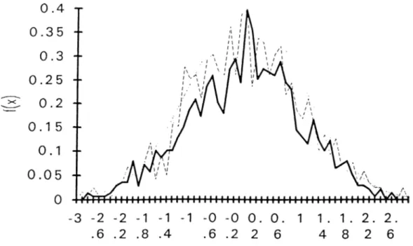
In the analysis o f this part, we will use errors which are distributed uniformly between -0.5 and 0.5. Mean o f errors is 0. Therefore, residuals are centered. We will depict the distribution o f S„ which is Monte Carlo distribution, (see Eq.2.2); S„* which is Bootstrap distribution (see Eq.2.8), and standard Normal distribution which represents Normal approximation based on CLT. Figure 2.2 depicts these curves. The curve with small lines ( _____) shows Monte Carlo. Solid line represents Bootstrap and curve with dots represents CLT approximation. Since Monte Carlo and Bootstrap give broken curves due to construction o f Histogram, we can not assess which method is better. However, in later section, we will introduce an efficient smoothing procedure.

2.4 Asymmetrically Distributed Errors

It is interesting to check what happens to the model when errors are asymmetrically distributed. We can assign many asymmetric distribution for errors. For this case, a simple trick is used for constructing asymmetric distribution. The distribution o f errors is composed by chopping distribution into half and derived errors in each half according to ~ N (0,1) and ~N(0,9) respectively. Hence we can construct a distribution which is asymmetric for usage in modelling.

Figure 2.2 Unsmoothed distribution o f S,„ S*„ and (j) for errors ~U(-0.5,0.5)

Actually, mean o f errors for this case inevitably shifted away from zero a little bit. This violates the centered residuals condition and so , it should be corrected. We can eliminate this drawback by subtracting all residuals from their mean. This will provide us to have centered residuals for the analysis. Figure 2.3 shows the distributed errors which is asymmetric.

Asymmetric distributed errors cause estimated P term to be distributed asymmetrically too. Since for asymmetric distributions because o f skewness, it is supposed that CLT Approximation diverges from accurate results. Because, structure o f Normal Approximation based on CLT is not suitable to catch skewness part o f unknown distribution. In this case. Bootstrap should work better and catch this asymmetry part where CLT Approximation fails.

A s y m m e t r i c E r r o r D i s t r i b u t i o n

Figure 2.3

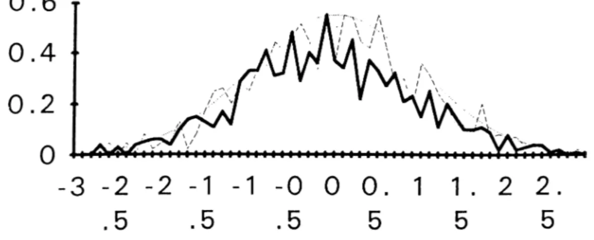
Considering above assumptions, we have to face that Bootstrap curve should be closer to Monte Carlo distribution curve. Figure 2.4 sketches the distributions o f Monte Carlo, Bootstrap and standard Normal for asymmetric distribution case.

B o o t s t r a p v s . N o r m a l

A p p . ( U n S m o o t h e d )

Figure 2.4 Distributions o f Sn, S*„ and (j) for asymmetrically distributed errors

It is seen that these broken lines do not give clear idea about how good Bootstrap estimation works from above figure. It is necessary to smooth these curves. The following section discusses how to smooth these curves.

2.5 Smoothing Procedure

So far, the comparison o f Normal Approximation and Bootstrap estimation was analytically investigated and computer simulations were performed. However, in the light o f curves derived by Monte Carlo simulations, it is difficult to predict which method is better than the other. Here, it is necessary to introduce a smoothing procedure to give clear vision o f comparison o f these curves. B .W .Silverm an, 1986, in his book called,

^'Density Esdmaiion For Statistics and Data Analysis”

introduced a smoothing procedure which is quite convenient for our model.

The problem o f choosing how much to smooth is o f crucial importance in density estimation. It should never be forgotten that the appropriate choice o f smoothing parameter will always be influenced by the purpose for which the density estimate is to be used.

Before passing through smoothing procedure, it should be chosen an appropriate kernel for unknown distribution. Kernel estimates should satisfy the condition

jA:(x).iZv =

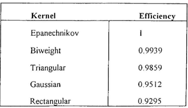
where usually, but not always, K will be a symmetric probability density. Silverman proposes many different kernel estimates to smooth density, but which kernel will be used is an important question to be considered. Below table (Table 2.1) gives the different types o f kernels and their efficiencies which is calculated out o f 1.

K ernel Efficiency Epanechnikov 1 Biweight 0.9939 Triangular 0.9859 Gaussian 0.9512 Rectangular 0.9295

Table 2.1 Some kernels and their efficiencies

It is seen from above table that all these kernels are quite efficient for estimation. In this model, G aussian kernel is chosen for smoothing procedure. The formula o f the Gaussian kernel is defined as

■^(0 - 2 ^

Note that it has same formula with standard Normal density. This will provide convenience in our analysis. Because, the distribution o f estimated P is converted to a distribution which has mean 0 and variance 1.

The working principle o f smoothing procedure is as follows. The kernel estimator is a sum o f "bumps" placed at the observations. Therefore, kernel function, K determines the shape o f bumps while the window width, denote as h, determines their width. When h tends to zero, kernel function spikes at the observations, but while h becomes large, all details, spurious and others, are obscured. Therefore, after choosing the suitable kernel, an appropriate window width should be calculated. Silverman has calculated the optimal window width for Gaussian kernel as"

See Silverman, pg 45

h=l .06 a n’’^’

In our model we proposed that variance is 1. Furthermore, sample size, n, has been chosen 100 before. Hence, appropriate window width is found as 0.422. Based on this values, the smoothing density function is defined as

nh ; - I h

where n and h are sample size and optimal window width respectively. X,'s are observations in sample data. Consequently, we can reach a smooth distribution by injecting Monte Carlo simulation results into above function.

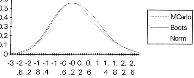
Figure 2.5 and 2.6 clearly depict the smoothed versions o f Sn, S*„ and (j) distribution for symmetrically and asymmetrically distributed errors respectively. Now, we can investigate

-3 -2 -2 -1 -1 -1 -0 -0 0. 0. 1 1. 1. 2. 2. .6 .2 .8 .4 .6 .2 2 6 4 8 2 6

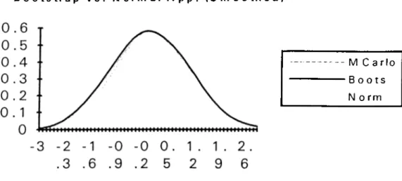
B o o t s t r a p v s . N o r m a l A p p . ( S m o o t h e d )

M Carl o • B o o t s

Nor m

Figure 2,6 Distribution o f S„, S*„ and cj) for asymmetrically distributed errors

the effect o f changes in regressor X. So far, when we use asymmetrically distributed errors, we have taken regressor X as 90% -1 or 1 and 10% -3.3 or 3.3. This provides X to be nonsymmetric. It can be interesting to investigate the behavior o f curves when regressor X is symmetric which takes either -1 or 1. Figure 2.7 depicts the case when X is symmetric.

B o o t s t r a p v s . N o r m a l A p p . ( S m o o t h e d )

M Carl o B o o t s No r m

Figure 2.7 Distribution o f S,„ S*„ and (j) when X is either -1 or 1

It is seen that when we use symmetric regressors, X, both Bootstrap and CLT approximation curves approach to Monte Carlo curve. Actually, from the figures, it may

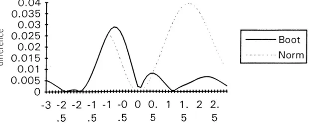
be difficult to predict which curve is closer than the other. Figure 2,8, 2.9 and 2.10 depict the difference between Bootstrap and Monte Carlo; CLT approximation and Monte Carlo.

. 5

. 5

. 5

5

5

5

F igure 2,8 Differences o f curves to Monte Carlo when errors are ~U(-0.5, 0.5)

•Boot Norm

.5

.5

.5

5

5

5

Figure 2.9 Differences o f curves to Monte Carlo when errors are asymmetrically distributed and X is asymmetric

•Boot

Norm

-3 -2 -2 -1 -1 -1 -0 -0 0. 0. 1 1. 1. 2. 2. .6 .2 .8 .4 .6 .2 2 6 4 8 2 6

Figure 2.10 Difference o f curves when errors are asym. distributed and X is symmetric We will introduce a key word, m axim um gap which is helpful in our analysis. It is defined as

S u p ( ! e n |f '’ -I^*l or SuppsR I f - cl)| (2.13)

Eq. 2.13 will provide a tool to comment on efficiencies o f estimation methods. In Figures 2.8, 2.9, 2.10, it is seen that Bootstrap works better than CLT Approximation. There are some points where CLT approximation curve is closer to Monte Carlo curve than Bootstrap. However, in most o f the points. Bootstrap approaches to Monte Carlo curve more than CLT approximation. In our analysis, the maximum gaps between curves clearly show that Bootstrap gives more correct results than CLT approximation. Because o f this, we can conclude that Bootstrap works better than Normal Approximation based on CLT. Below table (Table 2.2) indicates the methods and their maximum gaps for both

B ootstrap N orm al App.

Sym m etric D istribution 0.027182 0.037718

Asyin. Distr. when X is Symm. 0.020672 0.039569 Asym. Distr. when X is Asyniin. 0.057052 0.071729

Table 2.2 Methods and their maximum gaps

Maximum gaps also clearly validate that Bootstrap is more suitable to use. It will be misleading to use CLT approximation instead o f Bootstrap to estimate distribution.

2.6 An Example

The empirical analysis showed that the results are consistent with the results o f theoretical approach. However, it should be considered whether our analysis can be applied to real life statistics. The following analysis investigates an example data which is taken from the

Economic Report o f the President, 1984 pq 261.

The data contain per capita disposable income (Y) and per capita consumption expenditures for the period 1929- 1984. It is intended to estimate the consumption fijnction for United states from the data. However, during estimation, it is found that there are some outliers in data. During 1942-1945, the observations deviate from estimated results quite a lot. Therefore, these observations were all disregarded.

The analyses which were done before, derived that true beta term is 0.885 and intercept is 85.725. Based on these values , the formula o f fitted line is found as;

C,= 85.725 + 0.885 Yt

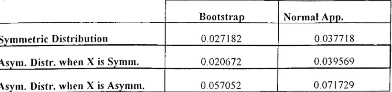
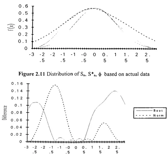
We will perform our analysis in the light o f these considerations. In this case, we will take intercept as known and try to estimate the coefficient in front o f disposable income for sake o f simplicity. Otherwise, X matrix becomes tx2 matrix which brings more work to do. Figure 2.11 clearly depicts the curves o f Sn, S*„ and (j) based on actual data. Monte Carlo curve (S„) is solid line. Bootstrap curve (S*n) is dotted line and CLT approximation curve is cutted line.

0 . 6 T 0 . 5 ·■ 0 . 4 ■· 0 . 3 ·· 0 . 2 · · 0 . 1 ·.' '■ 0 ¡4^ -3 -2 -2 .5 -0 0 0. .5 5 1 1 2 . 5 Figure 2.11 Distribution o f S,„ S*„, (j) based on actual data

-Boot Norm

Figure 2.12 Difference o f curves to Monte Carlo in real data

In Figure 2.1 1, the actual (Monte Carlo) distribution seems quite far away from being symmetric. We have proven that Bootstrap gives closer results than CLT approximation when distribution is asymmetric. In Figure 2.12, we see that Bootstrap is closer than CLT approximation in negative scale. But, on the other side, CLT approximation gives closer results than Bootstrap. Therefore, we have to look the maximum gap o f curves in order to understand which method is better than the other in overall look. We found that maximum gap between Monte Carlo and CLT approximation is 0.312485 which is higher than the gap between Monte Carlo and Bootstrap (i.e. 0.280967). Therefore, we can conclude that Bootstrap works better than CLT Approximation considering overall performance. This example validates our analysis on artificial data. We have found that in asymmetric distributions. Bootstrap gives closer results than Normal approximation based on CLT.

At the end o f our first application analysis, it is useful to check the behavior o f Bootstrap when data contain leverage point. We inserted a good leverage point to the data through matrix X and replaced one value which was 1 with 10.

.6 .2 .8 .4

.6 .2 2 6

4 8 2 6

F igure 2.12 Distribution o f S„, S*„ and (f) when data contain leverage point

From Figure 2.12, when data contain leverage points, the maximum gap between Bootstrap and Monte Carlo curves increases to 0.058985. The gap between CLT Approximation and Monte Carlo also increases to 0.059551. As a result, we can easily conclude that leverage point slightly affects the accuracy o f both Bootstrap and CLT Approximation. Nevertheless, Bootstrap still gives close results to Monte Carlo relative to CLT Approximation.

B o o t N o r m

Using Bootstrap in F-test

In the previous chapter, we have investigated the accuracy o f Bootstrapping and Normal Approximation based on CLT.

3.1 Bootstrapping F-test when Model is 1st order ADL

In this chapter, it is intended to investigate some further applications o f Bootstrap. In this section, we will mainly focus on using Bootstrap in F-test. F-test is a technique to test the significance o f regressors. F-test works exactly when the regressors are nonstochastic, i.e. Y|= p.Xi + Et. However, it has been proven that F-test asymptotically works when dynamic models are used. Precisely, F-test does not give true values when sample sizes are low. In this case, we can not use the table values as critical values o f F- test. M onte Carlo simulation results are the true critical values. On the other hand, these results are not available to the experimenter, because he should know the values o f true parameters (ao, ai 82) in order to compute critical values by Monte Carlo.

At this point, we use Bootstrap in order to compute critical values for different sample sizes. At first, we construct our model which is first order ADL model, i.e. Yt=ao.Xt+ai.Yt-i+a2.Xt-i+et and then , test whether Bootstrap would give close results to M onte Carlo simulation o f 95% significance level o f F-test. In our testing hypothesis, null

hypothesis is a i- 0 and a2=0 which restricts our dynamic model. On the other hand, alternative hypothesis is against null hypothesis, i.e. ai;^0 and

a

2^0 which is unrestricted

form o f the model.

The F-test statistic is derived as follows.

F =

( K - q , . X , f - \ \ } : - q , . X ,

-q.y_,

- a , . X , J

)/2

\ \ Y - a , . X - a , . Y , _ , - a , . X j l { t - A )

In the above equation, tilda (~) above ao denotes restricted maximum likelihood estimation o f the coefficient in front o f the Xt term under restriction ai=0 and a2=0. Meanwhile, the terms which have hat(^) above, are unrestricted maximum likelihood estimators. The critical value is the measure which depends on the significance level o f test and helps us to reject or accept the null hypothesis. If F-test gives smaller value than critical value then we accept null hypothesis otherwise we should reject it. The aim o f this thesis is to check that whether Bootstrap can be used in calculating critical value o f F-test or not. If so, this will give us an important facility in calculating critical value. That means, the necessity o f knowing the coefficient o f regressors disappears and estimated coefficients can also reach same results that we are seeking.

During this experiment, we will use 95% as significance level and hold Monte Carlo iteration size enormously high such as 60.000 in order to find the exact value o f critical value. After experiment, table 3.1 indicates the results for critical value o f F-test according to Monte Carlo, Bootstrap and Table (Asymptotic) depending on different sample sizes.

SA M P L E SIZE M O N T E C A RLO B O O T ST R A P TA B LE (Asymp.)

10 4.67794546 4.5606907 5.14

25 3.344504 3.3125865 3.47

50 3.1633513 3.1257652 3.21

100 3.0855887 3.0663446 3.08

T able 3.1 Critical Values o f F-test for different sample sizes

It is seen that M onte Carlo simulation results and asymptotic values become closer to each other when sample size is over 50. However, what we are concerned is whether B ootstrap approaches to exact values before size is 50. It is absolutely seen that Bootstrap technique also gives closer results to Monte Carlo results than table values when sample size is below 50. We observe that until sample size 50, we can use Bootstrap technique to find the critical value o f F-test. However, for the cases when size is bigger than 50, it is preferable to use asymptotic values (i.e. table values) since the problem in F-test because o f using dynamic models disappears. Moreover, after sample size 50, table values are more correct than Bootstrap values. Therefore, Bootstrap should be used when sample size is below 50 and left when size is over 50. Actually, sample size 50 may not be standard for F-test. It can change depending on regressor X. In later sections, we will concentrate on the effect o f change in regressors.

3.1.1 L everage Points Effect

We can also check the effect o f existance o f leverage points in the data set. This is actually checking the dependence o f Bootstrap technique on matrix X. Because, if B ootstrap diverges away from correct results when there are leverage points, then we have to leave using Bootstrap in F-test completely. Leverage points can be easily

generated by replacing the values o f robust data X with some uncorrelated values by hand. For the sake o f simplicity, we will investigate the effect o f good leverage points. Since, bad leverage points also affect the result o f Monte Carlo which is regarded as true value, we can not comment on rest o f the analysis correctly.

During the experiment, we inserted 10 value into matrix X where each variable in X was distributed as Normal with mean 0 and variance 1. If we rerun our program according to this consideration, we will get the following results;

S A M PL E SIZ E M O N T E C A R L O B O O T ST R A P TA B LE (Asymp.)

10 4.5910419 4.5226294 5.14

25 3.3464298 3.3185360 3.47

50 3.1128431 3.0782419 3.21

100 3.0447362 3.0168968 3.08

T able 3.2 Critical values o f F-test when data contain leverage points

When data contains leverage points inside, we see that for small sample size, the performance o f Bootstrap still looks quite good. As a result. Bootstrap can again be used in low sample sizes.Furthermore, leverage points do not change critical value o f F statistic much, and the accuracy o f Bootstrap stays still in considerable range. Therefore, generally, we can use Bootstrap in low sample sizes such as 10-50. However, table values that means asymptotic results gives better results when sample size is high such as over 50. Furthermore, existance o f leverage points does not affect the analysis.

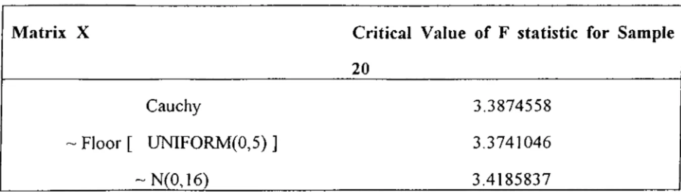
This opens a new idea to be investigated. Since leverage points do not affect critical value much , then it may be interesting to analyze the changes in critical value o f F-test when all regressor X changes. In this analysis, we chose sample size as 20 and search for the critical values o f F-test depending on different regressor X. Here, we

dropped M onte Carlo iteration size from 60,000 to 10,000. Because, it is not needed to put much emphasis on very accurate results. In the first run, we created regressor X in which values are distributed as Cauchy. In second run, we changed X to the floor o f uniformly distributed numbers between 0 and 5 and finally, in the third run, we created X distributed as ~ N (0 ,16). Based on these regressors, Monte Carlo simulation gave critical value o f F-test as below.

M atrix X C ritical V alue o f F statistic for Sam ple 20

Cauchy 3.3874558

~ Floor [ UNIFORM(0,5) ] 3.3741046

~ N (0,16) 3.4185837

T able 3.3 Critical value o f F statistic for different regressors X

Table 3.3 shows that critical value o f F-test does not completely depend on regressor X. The critical values are not changing too much as regressor X completely changes. This proves that F-test does not depend on regressor X much. Therefore, we can use F test whatever data X is.

3.2 Bootstrapping F-test when Model is 2nd Order ADL

After investigating the features o f Bootstrapping in first order ADL model, it is also intended to seek the changes in results when model is changed to second order ADL, i. e. Yt=ao. Xt+a 1. Xt-1+b 1. Yt-1 +32. Xt-2+b2. Yt-2+Si·

Now, if null and alternative hypothesis are constructed as follows;

Ho: a2=b2=0 vs. H i:a2i^0 and b2?^0

The aim o f including second order ADL model in the analysis, is to make the model more dynamic. In this case, the required sample size for correct value o f F statistic should increase. Furthermore, we will check the performance o f Bootstrapping when the order o f lag increases. After experiment, the critical values o f F test based on second order ADL model are derived at below table.

SA M PL E SIZE TA B LE M O N T E C A R L O B O O T ST R A P 10 5.79 11.857767 12.74724 15 4.10 5.5250613 5.0368244 25 3.49 3.8339534 3.9817073 50 3.22 3.4521521 3.5058512 100 3.11 3.0218225 3.1034317

T able 3.4 Critical values o f F when model is second order ADL

According to table 3.4, we see that there are two interesting results. The first one is, when sample size is 10, there is a big difference between asymptotic value and Monte Carlo value. Table value is absolutely incorrect. However, as sample size increases to 15, there occurs a sharp decrease in difference between asymptotic result and Monte Carlo result. Second interesting issue is, when model is changed to second order ADL model which is more dynamic than before, table values (which are asymptotic results) do not give correct results until sample size is over 100. Actually, even at sample size 100, Bootstrap gives more accurate result than asymptotic value.

Therefore, when our model is second order ADL, we should again use Bootstrap instead o f table values for low sample sizes (10-100). Table values become correct when sample size is sufficiently high (e.g. >100 ).

So far, we have investigated the usage o f Bootstrap technique in F-test. Consequently, Bootstrap gave better results than asymptotic values o f F-test when sample size is low. This is because o f dynamic nature o f the model. It is known that F-test is asymptotically true in dynamic models. Therefore, we can use Bootstrap in low sample sizes where F-test does not work.

Using

Bootstrap

in

Common

Factor

Restrictions

4.1 Using Bootstrap in COMFAC restrictions

In this chapter, we will use Bootstrap to test common factor restrictions. Suppose that our model is taken as follows;

Y ,= a.X ,+ p.Y ,.,+ Y .X ,.,+ E , (4.1)

To test common factor restriction, we propose testing hypotheses as follows;

H o;y=-a.3 vs. Hi.y^i^-a.p

Null hypothesis denotes that model has common factor, while alternative one denotes that model does not have a common factor and can be treated as linear one. The term y can be regarded as actual coefficient o f regressor X u . The comparison criteria for tests with common factor should be reconsidered. It is appropriate to use pow er curves o f tests to test their efficiencies. Since there is a possibility o f being nonlinear for our model, we can not use the F-test for this case. Therefore, we intend to use likelihood ratio test for testing nonlinear models. In this test, LR statistic would give the ratio o f likelihood functions o f the model for tw o different hypotheses. For the null hypothesis, it can be difficult to guess the parameters, (a,P ) simultaneously which maximize the likelihood function. Therefore,

it is more appropriate to find these parameters by fixing one and finding the other parameter which maximizes likelihood, and then, changing the fixed parameter according to both parameters maximize likelihood function at global maximum value. Equation can be written as follows.

^ S u p \\Y ,- a . X , - p . l_ , + a .p . X , _ , \f

Su p \\Y ,-d .x,-fi.Y ,^ ,-y\x,_,\f

In Eq.4.2, the parameters which have tilda (~) above, denotes the restricted maximum likelihood estimates. On the other hand, the parameters which have hat

(^)

above, denotes the unrestricted maximum likelihood estimates.

Throughout this analysis, we will define Bootstrap as follows. At first, the parameters, a~, P~ are estimated by restricted ML. Furthermore, a , and are estimated by unrestricted ML. Then, dependent variable, Yt, is produced by using estimated parameters. We denote new dependent variable as Yt*. Bootstrapped LR is obtained from Eq.4.2 by replacing Yi* instead o f Yt.

Finally, it is worthwhile to discuss about another testing technique for common factor, called W ald T est'^. This test is quite simple and rather efficient. The testing hypotheses for the Wald test are as follows ;

H o :W = 0 vs H , ; W? ^ 0

where W stands for Wald statistic. Actually, there are many derivation formula for W. In this thesis, we will simply find W as follows.

L et’s define f(.) as

f(.)= y + a. p

12_{See G.Kemp (1991) for comicx Wald tests with application to COMFAC tests}

These three parameters are derived from unrestricted maximum likelihood estimation. By dividing f(.) value into its standard deviation , Wald statistic can be derived easily.

W = f ( . ) / [ v a r ( f ( . ) ) l ' ^

In empirical analysis part, we constructed our model as follows: Y,=a.Xi+p.Yt-i - a.p.Xt-i. As it is seen that the coefficient in front o f X u is the multiplication o f other coefficients o f other regressors with minus sign. Therefore, there is a common factor in the model. This model was firstly discussed by Sargan. Afterwards, H endry and M izon put some empirical analysis on this model. However, so far, there has been not so much analyses on using Bootstrap method on common factor models.

We will investigate the efficiencies o f three different methods.

Likelihood Ratio,

Bootstrap and Wald.

As we mentioned before, we are going to use simple Wald statistic. Reader may refer to studies o f Hendry and M i z o n f o r more complex Wald statistics. Our hypotheses are;

Ho:Y+a.p=0 vs. Hi:y+a.p?iO

During the experiment, we have derived that 95% critical values for LR, Bootstrap and Wald are 4.0612399, 5.1852510 and 1.6411099 respectively. Actually, these critical values are not standard for all tests. They also depend on regressor X. That means there is no a certain critical value to be looked for as in F-test. Therefore, we have to use other comparison mechanisms to check the performance o f tests. It is convenient to use Pow er C urves o f each test.

We have used N eym an-Pearson to construct Power Envelope. We obtain Neyman-Pearson by dividing the probability density o f Yt under alternative hypothesis by the probability density o f Yt under null hypothesis. Now, our testing hypotheses become.

Ho: Y-Hx.p=0 vs. Hi : y + a .p = ^ > 0

In figure 4.1, Pow er curve o f each test has been derived.

...- LR

— _{- — Wald}

Power E.

Figure 4.1 Power Curves o f Wald, LR and Bootstrap

In the above figure, Wald test gives the closest power curve to the power envelope. That means Wald test provides more powerful tool in common factor restriction models. There is no need to use Bootstrap or LR test. In Figure 4.2, we can see the differences o f tests to power envelope. The difference between Wald test and power envelope is minimum. LR works worser than Wald test but better than Bootstrap. Bootstrap is the worst test in our analysis.

So far, we have generated regressor X as values between -5 and 5. To see leverage point effect, by replacing one value o f X with 20, we generated a good leverage point in data set. For this case, LR and Wald test give approximately same performance. Again, Bootstrap is worst test in the analsysis. Figure 4.3 depicts the difference between tests and power envelope.

Figure 4.2 Differences between tests and power envelope

Figure 4.3 Differences between tests and power envelope when data have leverage point

Figure 4.3 shows that Wald and LR give very close power curves when data contain leverage point. The differences between these tests and power envelope are almost same. We see that Bootstrap still works bad relative to other tests.

In next section, we will analyze a new technique which increases the performance o f Bootstrap.

4.2 Bootstrap-Bartlett Correction

During empirical analysis, we have found that straightforward Bootstrap test gives w orser answers than other tests. Furthermore, power curve calculation o f Bootstrap seems to be cumbersome both for programmer and computer. We will introduce a technique which brings easiness and accuracy in calculation. It is called B ootstrap- B a rtle tt C orrection. This technique decreases necessary iteration size considerably low and finds more accurate results with respect to straightforward Bootstrap.

Before passing to issue, we know that -2 log LR asymptotically converges to x^f where f is the degrees o f freedom*“*. Since COMFAC puts one restriction on parameters, it can be shown that LR test is asymptotically Chi-Square distribution with degrees o f freedom 1. If we sufficiently obtain LR statistics, the average o f them will converge to 1 since the mean o f Chi-Square distribution is 1. However, for low iteration sizes, this value may be away from 1. This is also true for using Bootstrap in LR statistic. We will use this fact in Bartlett correction. We define this correction by using following algorithm.

SlepI:

Generate 100 H=-2 log LR by using Bootstrap, (i.e. H*', H V

5'/e/?2.· Average these and get the expected value o f that sample.( Say M=(H*‘+...+H *'® >100).

Step3:Dti\x\Q

new H, say H ’, as H ’= H / M.

Step4:'^otQ

that H ’ will automatically have expected value 1 which matches the large sample value. Finally, reject null hypothesis if H ’>c where c is critical value ofx^i .

Now, we will analyze its empirical application. Before, passing Bootstrap Bartlett issue, let’s investigate the asymptotic behavior o f LR. If we check for the mean o f LR for

14_{This can be easily found by Taylor series expansion around 0}

different sizes, we see that as size increases, mean o f LR gradually converges to 1 (See Table 4 .1 ) SA M PL E SIZE M EAN 50 1.5616565 100 1.4489513 500 1.3886276 1000 1.2477456

T able 4.1 Mean o f LR depending on sample size

Now, if we apply Barlett correction method on Bootstrap, we provide our sample to converge to Chi-Square with degrees o f freedom 1 faster than straightforward Bootstrap. By using Bartett correction, we both decrease the iteration size from 1000 to 100 which brings speed in calculation and obtain more accurate result than straightforward Bootstrap. It is seen that mean o f -2 log LR is still larger than 1 when sample size is 1000. ( See table 4.1). Therefore, -2 log LR hasn’t converge to Chi-Square distribution yet. However, by Bootstrap-Bartlett correction, we have obtained the results which have mean 1 which is same as Chi-Square distribution with degrees o f freedom 1. Therefore, we have approached to Chi-Square distribution faster than before. Because o f this, critical value o f Bootstrap which was 5.18 in straightforward Bootstrap decreased to 3.7677999 which is quite close to critical value o f χ^ı which is 3.84. From the theoretical analysis, we should obtain more close curves to the power envelope. When we rerun the program according to Bartlett correction, we will get the power curves o f Bootstrap-Bartlett and straightforward Bootstrap as;

Figure 4.4 Power curve o f Bootstrap-Bartlett and StrFwd. Bootstrap

In Figure 4.4, we see that power curve o f Bootstrap has been improved a little bit. That means, Bartlett correction increases the power curve o f Bootstrap. The difference between power envelope and Bootstrap decreases. (See Figure 4.5). However, this decrease is not so large to dominate Wald test.

■Boot Barlett

Figure 4.5 Differences between Bootstrap (StrFwd,Bartlett) powers and power envelope