Journal of Computational and Applied Mathematics

Örnek: Beceri Temelli

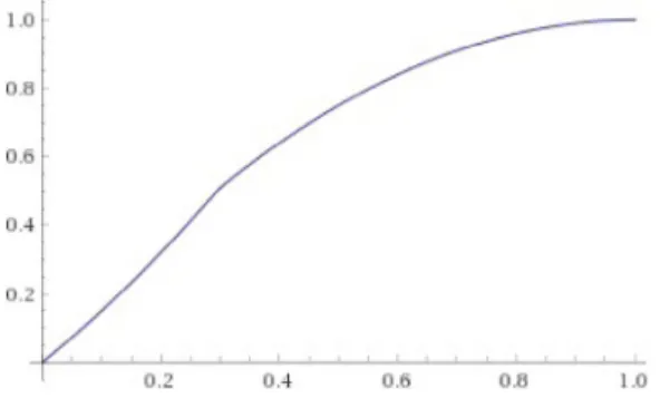
A next step is the construction of the distribution of the concomitants of order statistics for the presented Pseudo–Gompertz distribution and the derivation of the survival and

Joint probability function for the variables of surplus immediate before ruin, deficit at ruin and time to ruin is obtained and potential applications of it are discussed. It

The north–south quantile points, NSQP, approach for the computation of the quantiles of random loss variables can be efficiently utilized in order to model bivariate dependent

The proposed bivariate pseudo-Gompertz distribution has the complacency for the survival and hazard modeling and their extensions to the applications besides reliability analysis

This special issue has been realized in connection with the International Conference on Applied and Computational Mathematics (ICACM, http://icacm.iam.metu.edu.tr/ ) that was held

Conclusion: No statistically significant difference between the groups in terms of genital hygiene behaviors was evident, as the results of the study showed that the average of

Non-Blind: This technique needs the original cover image to discover and extract the watermark, some watermark techniques of this type is called the private as it refers to

References

[1] A.C. Aitken, H.T. Gonin, On fourfold sampling with and without replacement, Proc. Roy. Soc. Edinburgh 55 (1935) (1935) 114–125.
[2] M.A. Hamdan, Canonical expansion of the bivariate binomial distribution with unequal marginal indices, Internat. Statist. Rev. 40 (1972) 277–288.
[3] M.A. Hamdan, D.R. Jensen, A bivariate binomial distribution and some applications, Aust. J. Stat. 18 (1976) 163–169. [4] S. Kocherlakota, K. Kocherlakota, Bivariate Discrete Distributions, Marsell Dekker, Inc., New York, 1992.
[5] I. Bairamov, O. Elmastas Gultekin, Discrete distributions connected with bivariate binomial, Hacet. J. Math. Stat. 39 (1) (2010) 109–120. [6] I. Bayramoglu, G. Kemalbay, Some novel discrete distributions under fourfold sampling schemes and conditional bivariate order statistics, J.
Comput. Appl. Math. 248 (2013) 1–14.
(10)
[8] Drgabriel Escarela, Jacques F. Carriére, A bivariate model of claim frequencies and severities, J. Appl. Stat. 33 (8) (2006) 867–883.
[9] A. Castaño-Martínez, G. Pigueiras, M.A. Sordo, On a family of risk measures based on largest claims, Insurance Math. Econom. 86 (2019) 92–97. [10] R.E. Barlow, F. Proschan, Statistical Theory of Reliability and Lifetesting, Holt, Rinehart & Winston., New York, 1975.
[11] M. Tavangar, I. Bairamov, On conditional residual lifetime and conditional inactivity time of k-out-of-n systems, Reliab. Eng. Syst. Saf. 144 (2015) 225–233.
[12] K.B. Kavlak, The mean wasted life time of a component of system, J. Comput. Appl. Math. 305 (2016) 44–54.
[13] S. Eryilmaz, Reliability analysis of systems with components having two dependent subcomponents, Comm. Statist. Simulation Comput. 46 (2017) 8005–8013.
Şekil
Fig. 1. The graph of P { W n : n ≤ x | ζ 1 = k } for n = 5 , k = 3 , t = 0 . 5. Then P { W r : n ≤ x | n ∑ i = 1 ξ i = k } = ∑ ni = r ∑ min(i , k)j= max(0 , k + i − n) ( nj )( n − ji−j )( n − ik− j ) p 11j p i 12− j p 21k − j p n 22 − k − i + j ( n k ) F k
Fig. 2. The graph of FW t (x) given in (19) for t = 0 . 3.
Fig. 3. The graph of MRL functions for F 1 (x), F 2 (x) and. F W (x) Ψ F 1 (s) = MRL1, Ψ F 2 (s) = MRL2 and Ψ W t (s) = MRL3 for t = 0
Referanslar
Benzer Belgeler