Proceedings of the 2010 Industrial Engineering Research Conference
Analytic Network Process (ANP) for solar power plant location
problem
Zeki Ayag, Funda Samanlioglu,
Department of Industrial Engineering
Kadir Has University, Cibali, Istanbul 34083, TURKEY
Abstract
Solar energy is the most readily available source of energy, and one of the most important sources of the renewable energy, because it is non-polluting and helps in lessening the greenhouse effect. Main problem of establishing a solar power plant is to determine its location. In the presence of many location alternatives and evaluation criteria, a multiple-criteria decision making problem arises. In this work, the location problem will be solved by using Analytic Network Process (ANP) to figure out the most satisfying alternative. A numerical example is also included to show the proposed methodology in Turkey.
Keywords: Solar energy, multiple criteria decision making, analytic network process
1. Introduction
Every day, the sun sends out an enormous amount of energy, called solar energy. It radiates more energy in one second than the world has used since time began. This energy comes from within the sun itself. Like most stars, the sun is a big gas ball made up mostly of hydrogen and helium gas. The sun makes energy in its inner core in a process called nuclear fusion. Only a small part of the solar energy that the sun radiates into space ever reaches the earth, but that is more than enough to supply all our energy needs. Every day enough solar energy reaches the earth to supply our nation’s energy needs for a year. It takes the sun’s energy just a little over eight minutes to travel the 93 million miles to earth. Solar energy travels at a speed of 186,000 miles per second, the speed of light. Today, people use solar energy to heat buildings and water and to generate electricity. Solar energyhas great potential for the future. Solar energy is free, and its supplies are unlimited. It does not pollute or otherwise damage the environment. It cannot be controlled by any one nation or industry. If we can improve the technology to harness the sun’s enormous power, we may never face energy shortages again.
Solar power plant location problem is typical multiple-criteria decision making (MCDM) problem in the presence of various selection criteria and a set of possible alternatives. Among the available multi-attribute approaches, only the analytic hierarchy process (AHP) approach, first introduced by Saaty [1] has the capabilities to combine different types of criteria in a multi-level decision structure to obtain a single score for each alternative to rank the alternatives [2]. In AHP, a hierarchy considers the distribution of a goal amongst the elements being compared, and judges which element has a greater influence on that goal. In reality, a holistic approach like analytic network process (ANP), a more general form of AHP is needed if all attributes and alternatives involved are connected in a network system that accepts various dependencies. Several decision problems cannot be hierarchically structured because they involve the interactions and dependencies in higher or lower level elements. Not only does the importance of the attributes determine the importance of the alternatives as in AHP, but the importance of alternatives themselves also influences the importance of the attributes. In conventional ANP developed by Saaty, the pair wise comparisons for each level with respect to the goal of the best alternative selection are conducted using a nine-point scale of Saaty [3].
In literature, to the best of our knowledge, a number of studies have been realized in various fields using the ANP since it first was introduced by Saaty [4]. Some of them are presented here; Hamalainen and Seppalainen [5] presented ANP-based framework for a nuclear power plant licensing problem in Finland. They used the pair wise comparison process with the consistency index to determine the weightings of the alternatives. ANP is also used to incorporate product lifecycle in replacement decisions. The multi-attribute, multi-period model handles vital dynamic factors as well as interdependence among system attributes. The system attributes’ relative importance
which vary during the different stages of product life-cycle is captured in this model [6]. Meade and Presley [7] used the ANP method for R&D project selection. Agarwal and Shankar [8] presented a framework for selecting the trust-building environment in e-enabled supply chain. Lee and Kim [9] proposed an integration model by integrating the ANP and goal programming for interdependent information system project selection. Yurdakul [10] used the ANP method to measure long-term performance of a manufacturing company. Aragone´s-Beltran et al.[11] also suggested an ANP-based approach for the selection of photovoltaic solar power plant investment projects.
In this paper, an intelligent approach to solar power plant location problem through ANP is proposed to find out the best satisfying solar power plant location alternative. In addition, to prove the applicability of the proposed approach, a numerical example is presented.
2. ANP-based approach to solar power plant location problem
The schematic representation of the ANP-based framework and its decision environment related to solar power plant location selection is shown in the section of the case study. The overall objective is to find out the best location alternative. Firstly, the elements used in the ANP network are determined. These elements are very critical at the stage of the evaluation, and should be well-defined due to the fact that they play important role in finding out the best alternative out of the available options.
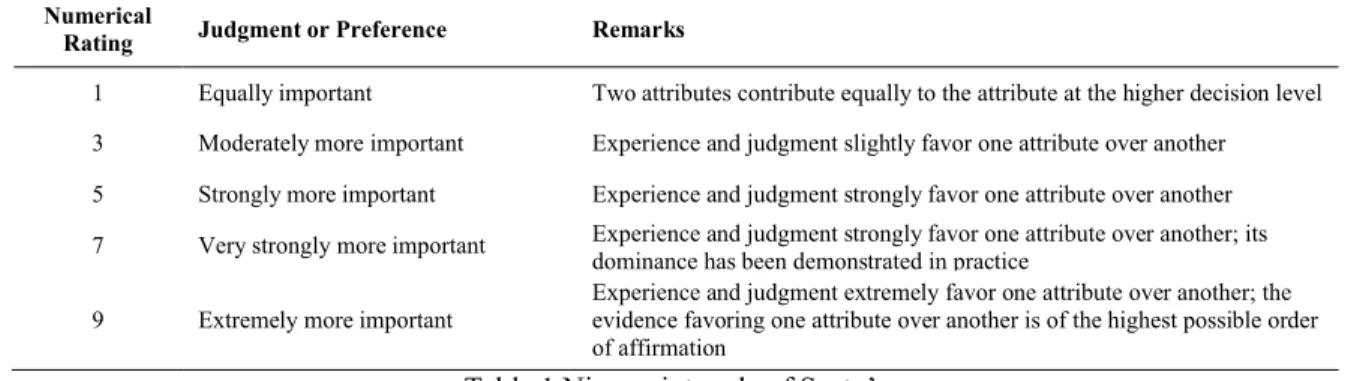
For representation of pair wise comparison, firstly, the network of solar power plant location selection should be established. The ANP method represents relationships hierarchically but does not require as strict a hierarchical structure and therefore allows for more complex interrelationships among the decision levels and attributes. After constructing flexible hierarchy, the decision-maker(s) is asked to compare the elements at a given level on a pair wise basis to estimate their relative importance in relation to the element at the immediate proceeding level. In conventional ANP, the pair wise comparison is made by using a ratio scale. A frequently used scale is the nine-point scale developed by Saaty [3] which shows the participants` judgments or preferences. Table 1 shows this fundamental nine-point scale.
Numerical
Rating Judgment or Preference Remarks
1 Equally important Two attributes contribute equally to the attribute at the higher decision level 3 Moderately more important Experience and judgment slightly favor one attribute over another 5 Strongly more important Experience and judgment strongly favor one attribute over another 7 Very strongly more important Experience and judgment strongly favor one attribute over another; its
dominance has been demonstrated in practice 9 Extremely more important
Experience and judgment extremely favor one attribute over another; the evidence favoring one attribute over another is of the highest possible order of affirmation
Table 1.Nine-point scale of Saaty’s
To obtain an understanding of the ANP methodology for solar power plant location selection problem, the six steps are presented as follows;
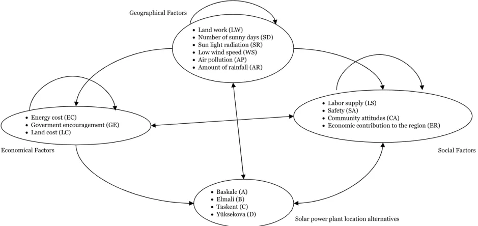
Step I. Model construction and problem structuring: In a typical ANP network, the problem is defined using clusters and the element inside each cluster. The network also defines the relationships and feedbacks among clusters, and among the elements in each cluster, if applicable. The ultimate objective of the network is to identify for finding out best alternative. In this study, we constructed ANP network diagram shown in Figure 1 for solar power plant location problem. The network has four clusters, three of which includes the groups of evaluation criteria, and one of which is the clusters of the location alternatives.
Step II. Building pairwise comparison matrices: By using nine-point scale of Saaty (table 1), the decision-maker(s) are asked to respond to a series of pairwise comparisons with respect to an upper level “control” criterion. These are conducted with respect to their relevance importance towards the control criterion. In the case of interdependencies, components in the same level are viewed as controlling components for each other. Levels may also be interdependent. The nine-point scale is used to compare two components, with a score of 1 representing indifferences between two components and 9 being an overwhelming dominance of the component under
Ayag, Samanlioglu
consideration over the comparison component. When scoring is conducted for a pair, a reciprocal value is automatically assigned to the reverse comparison within the matrix. That is, if
a
ij is a matrix value assigned to the relationship of componenti
to componentj
, thena
ij is equal to1
/
a
ji ora
ji
1
. Once the pair wise comparisons are completed, the local priority vectorw
(also referred as e-Vector) is computed as the unique solution to;Aw
maxw
(Equation 1), where,
max is the largest eigenvalue of A, A is a pairwise decision matrix made by using nine point scale.Step III. Checking out consistency ratios (CR) for pairwise comparison matrices: After constructing all pair wise matrices, for each of them, the consistency ratio (CR) should be calculated. The deviations from consistency are calculated by using Equation 2; the measure of inconsistency is called the consistency index (CI);
1
max
n
n
CI
, where n is the size of A (Equation 2). The CR is used to estimate directly the consistency of pairwise comparisons, and computed by dividing the CI by a value obtained from a table of Random ConsistencyIndex (RI), the average index for randomly generated weights [1] (Equation 3);
RI
CI
CR
(Equation 3). If the CR is less than 10%, the comparisons are acceptable, otherwise they are not.Step IV. Pair wise comparison matrices of inter-dependencies: In order to reflect the interdependencies in the network, pairwise comparisons among all the criteria are constructed and their consistency ratios are calculated as we previously defined in Step II and Step III.
Step V. Super-matrix formation and analysis: The super-matrix formation allows a resolution of the effects of interdependence that exists between the elements of the system. The super-matrix is a partitioned matrix, where each sub-matrix is composed of a set of relationships between two levels in the graphical model. Three types of relationships may be encountered in this model; (1) independence from succeeding components, (2) interdependence among components, (3) interdependence between levels of components. Raising the super-matrix to the power 2k+1, where k is an arbitrary large number, allows convergence of the interdependent relationships between the two levels being compared. The super-matrix is converged for getting a long-term stable set of weights.
Step VI. Selection of the best solar power plant alternative: After the super-matrix is converged for getting a long-term stable set of weights, the best alternative with highest weight is delong-termined in the super-matrix.
3. Numerical example
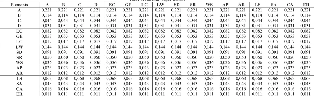
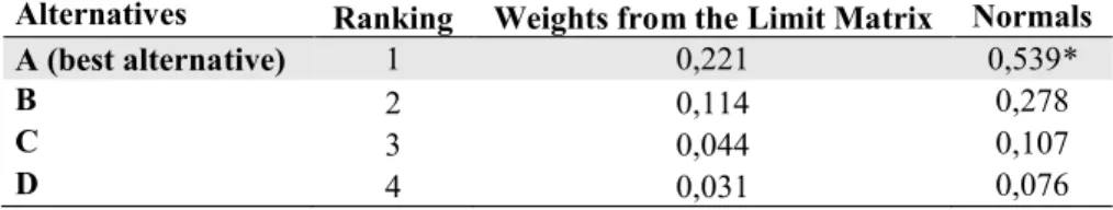
In this paper, we will find out the best location of solar power plants for Turkey in terms of a set of evaluation criteria. In figure 2, the network diagram shows four different clusters, including a cluster of the location alternatives. The alternatives named location A, B, C, and D were determined as shown in figure 1. To construct the super-matrix including all the feedback and the relations in the network, the nine point scale of Saaty’s as given in table 1, is used to make pairwise comparisons. An example of this pairwise matrix using Equations 1-3 is given in table 2 to show for the readers. In table 3, the un-weighted super-matrix is given to show all the relationships in the network for the location problem. In addition, the data indicated in table 4 showing the weights of the clusters is used to calculate the weighted super-matrix, shown in table 5. Finally, table 6 and 7 shows the limit matrix to find out the best alternative. Obviously, the location A is the best alternative with highest weight (0,539).
Table 2.Pair wise comparison matrix for the relative importance of the criteria for Location A under the cluster, Social Factors (CR=0.043) A LS SA CA ER e-Vector LS 1.000 1.000 5.000 9.000 0.488 SA 1.000 1.000 3.000 3.000 0.330 CA 0.200 0.333 1.000 1.000 0.096 ER 0.111 0.333 1.000 1.000 0.086
Energy cost (EC)
Goverment encouragement (GE) Land cost (LC)
Land work (LW)
Number of sunny days (SD) Sun light radiation (SR) Low wind speed (WS) Air pollution (AP) Amount of rainfall (AR) Geographical Factors
Solar power plant location alternatives Labor supply (LS) Safety (SA)
Community attitudes (CA)
Economic contribution to the region (ER)
Social Factors Economical Factors Baskale (A) Elmali (B) Taskent (C) Yüksekova (D)
Ayag, Samanlioglu
Table 3.The un-weighted super-matrix
Elements A B C D EC GE LC LW SD SR WS AP AR LS SA CA ER A 0.000 0.000 0.000 0.000 0.636 0.608 0.627 0.459 0.488 0.581 0.477 0.513 0.592 0.602 0.519 0.526 0.488 B 0.000 0.000 0.000 0.000 0.177 0.172 0.198 0.388 0.330 0.221 0.269 0.267 0.202 0.243 0.296 0.338 0.330 C 0.000 0.000 0.000 0.000 0.115 0.122 0.119 0.072 0.096 0.151 0.184 0.101 0.154 0.105 0.105 0.070 0.096 D 0.000 0.000 0.000 0.000 0.072 0.098 0.056 0.081 0.086 0.048 0.069 0.119 0.052 0.050 0.079 0.066 0.086 EC 0.000 0.000 0.000 0.000 0.000 0.833 0.500 0.748 0.724 0.511 0.509 0.669 0.643 0.487 0.509 0.748 0.474 GE 0.000 0.000 0.000 0.000 0.750 0.000 0.500 0.180 0.193 0.389 0.421 0.267 0.283 0.435 0.422 0.180 0.474 LC 0.000 0.000 0.000 0.000 0.250 0.167 0.000 0.071 0.083 0.100 0.070 0.064 0.074 0.078 0.070 0.072 0.052 LW 0.417 0.452 0.439 0.387 0.000 0.000 0.000 0.000 0.385 0.433 0.508 0.451 0.566 0.000 0.000 0.000 0.000 SD 0.243 0.248 0.252 0.273 0.000 0.000 0.000 0.508 0.000 0.291 0.265 0.339 0.258 0.000 0.000 0.000 0.000 SR 0.141 0.119 0.123 0.159 0.000 0.000 0.000 0.195 0.305 0.000 0.110 0.100 0.076 0.000 0.000 0.000 0.000 WS 0.100 0.088 0.106 0.089 0.000 0.000 0.000 0.155 0.173 0.154 0.000 0.077 0.057 0.000 0.000 0.000 0.000 AP 0.066 0.062 0.040 0.051 0.000 0.000 0.000 0.106 0.100 0.086 0.082 0.000 0.043 0.000 0.000 0.000 0.000 AR 0.033 0.032 0.040 0.041 0.000 0.000 0.000 0.037 0.037 0.034 0.035 0.033 0.000 0.000 0.000 0.000 0.000 LS 0.488 0.519 0.488 0.477 0.540 0.513 0.526 0.614 0.435 0.466 0.449 0.558 0.573 0.000 0.643 0.692 0.703 SA 0.330 0.296 0.330 0.269 0.306 0.267 0.338 0.197 0.373 0.357 0.364 0.263 0.210 0.669 0.000 0.231 0.174 CA 0.096 0.105 0.096 0.185 0.087 0.101 0.070 0.139 0.114 0.123 0.128 0.122 0.159 0.267 0.283 0.000 0.123 ER 0.086 0.079 0.086 0.069 0.067 0.119 0.066 0.050 0.078 0.055 0.060 0.057 0.058 0.064 0.074 0.077 0.000
Table 4.The cluster priority matrix
Clusters Alternatives Economical factors Geographical factors Social factors
Alternatives 0.000 0.649 0.614 0.669
Economical factors 0.000 0.295 0.197 0.267
Geographical factors 0.750 0.000 0.139 0.000
Social factors 0.250 0.057 0.050 0.064
Table 5.The weighted super-matrix Elements A B C D EC GE LC LW SD SR WS AP AR LS SA CA ER A 0.000 0.000 0.000 0.000 0.413 0.395 0.407 0.282 0.300 0.357 0.293 0.315 0.363 0.403 0.347 0.352 0.326 B 0.000 0.000 0.000 0.000 0.115 0.112 0.129 0.238 0.203 0.136 0.165 0.164 0.124 0.163 0.198 0.226 0.221 C 0.000 0.000 0.000 0.000 0.075 0.079 0.077 0.044 0.059 0.093 0.113 0.062 0.095 0.070 0.070 0.047 0.064 D 0.000 0.000 0.000 0.000 0.047 0.064 0.036 0.050 0.053 0.029 0.042 0.073 0.032 0.033 0.053 0.044 0.058 EC 0.000 0.000 0.000 0.000 0.000 0.246 0.148 0.147 0.143 0.101 0.100 0.132 0.127 0.130 0.136 0.200 0.127 GE 0.000 0.000 0.000 0.000 0.221 0.000 0.148 0.035 0.038 0.077 0.083 0.053 0.056 0.116 0.113 0.048 0.127 LC 0.000 0.000 0.000 0.000 0.074 0.049 0.000 0.014 0.016 0.020 0.014 0.013 0.015 0.021 0.019 0.019 0.014 LW 0.313 0.339 0.329 0.290 0.000 0.000 0.000 0.000 0.054 0.060 0.071 0.063 0.079 0.000 0.000 0.000 0.000 SD 0.182 0.186 0.189 0.205 0.000 0.000 0.000 0.071 0.000 0.040 0.037 0.047 0.036 0.000 0.000 0.000 0.000 SR 0.106 0.089 0.092 0.119 0.000 0.000 0.000 0.027 0.042 0.000 0.015 0.014 0.011 0.000 0.000 0.000 0.000 WS 0.075 0.066 0.080 0.067 0.000 0.000 0.000 0.022 0.024 0.021 0.000 0.011 0.008 0.000 0.000 0.000 0.000 AP 0.050 0.047 0.030 0.038 0.000 0.000 0.000 0.015 0.014 0.012 0.011 0.000 0.006 0.000 0.000 0.000 0.000 AR 0.025 0.024 0.030 0.031 0.000 0.000 0.000 0.005 0.005 0.005 0.005 0.005 0.000 0.000 0.000 0.000 0.000 LS 0.122 0.130 0.122 0.119 0.031 0.029 0.030 0.031 0.022 0.023 0.022 0.028 0.029 0.000 0.041 0.044 0.045 SA 0.083 0.074 0.083 0.067 0.017 0.015 0.019 0.010 0.019 0.018 0.018 0.013 0.011 0.043 0.000 0.015 0.011 CA 0.024 0.026 0.024 0.046 0.005 0.006 0.004 0.007 0.006 0.006 0.006 0.006 0.008 0.017 0.018 0.000 0.008 ER 0.022 0.020 0.022 0.017 0.004 0.007 0.004 0.003 0.004 0.003 0.003 0.003 0.003 0.004 0.005 0.005 0.000
Table 6.The limit super-matrix
Elements A B C D EC GE LC LW SD SR WS AP AR LS SA CA ER A 0,221 0,221 0,221 0,221 0,221 0,221 0,221 0,221 0,221 0,221 0,221 0,221 0,221 0,221 0,221 0,221 0,221 B 0,114 0,114 0,114 0,114 0,114 0,114 0,114 0,114 0,114 0,114 0,114 0,114 0,114 0,114 0,114 0,114 0,114 C 0,044 0,044 0,044 0,044 0,044 0,044 0,044 0,044 0,044 0,044 0,044 0,044 0,044 0,044 0,044 0,044 0,044 D 0,031 0,031 0,031 0,031 0,031 0,031 0,031 0,031 0,031 0,031 0,031 0,031 0,031 0,031 0,031 0,031 0,031 EC 0,082 0,082 0,082 0,082 0,082 0,082 0,082 0,082 0,082 0,082 0,082 0,082 0,082 0,082 0,082 0,082 0,082 GE 0,053 0,053 0,053 0,053 0,053 0,053 0,053 0,053 0,053 0,053 0,053 0,053 0,053 0,053 0,053 0,053 0,053 LC 0,017 0,017 0,017 0,017 0,017 0,017 0,017 0,017 0,017 0,017 0,017 0,017 0,017 0,017 0,017 0,017 0,017 LW 0,144 0,144 0,144 0,144 0,144 0,144 0,144 0,144 0,144 0,144 0,144 0,144 0,144 0,144 0,144 0,144 0,144 SD 0,091 0,091 0,091 0,091 0,091 0,091 0,091 0,091 0,091 0,091 0,091 0,091 0,091 0,091 0,091 0,091 0,091 SR 0,050 0,050 0,050 0,050 0,050 0,050 0,050 0,050 0,050 0,050 0,050 0,050 0,050 0,050 0,050 0,050 0,050 WS 0,036 0,036 0,036 0,036 0,036 0,036 0,036 0,036 0,036 0,036 0,036 0,036 0,036 0,036 0,036 0,036 0,036 AP 0,023 0,023 0,023 0,023 0,023 0,023 0,023 0,023 0,023 0,023 0,023 0,023 0,023 0,023 0,023 0,023 0,023 AR 0,012 0,012 0,012 0,012 0,012 0,012 0,012 0,012 0,012 0,012 0,012 0,012 0,012 0,012 0,012 0,012 0,012 LS 0,068 0,068 0,068 0,068 0,068 0,068 0,068 0,068 0,068 0,068 0,068 0,068 0,068 0,068 0,068 0,068 0,068 SA 0,043 0,043 0,043 0,043 0,043 0,043 0,043 0,043 0,043 0,043 0,043 0,043 0,043 0,043 0,043 0,043 0,043 CA 0,016 0,016 0,016 0,016 0,016 0,016 0,016 0,016 0,016 0,016 0,016 0,016 0,016 0,016 0,016 0,016 0,016 ER 0,011 0,011 0,011 0,011 0,011 0,011 0,011 0,011 0,011 0,011 0,011 0,011 0,011 0,011 0,011 0,011 0,011
Proceedings of the 2010 Industrial Engineering Research Conference
Table 7.The final table for the location alternatives
Alternatives Ranking Weights from the Limit Matrix Normals
A (best alternative) 1 0,221 0,539*
B 2 0,114 0,278
C 3 0,044 0,107
D 4 0,031 0,076
4. Conclusions and Future Research
In this paper, an ANP-based methodology for solar power plant location selection problem has been proposed by taking into consideration quantitative and qualitative elements to evaluate the location alternatives. As compared to the AHP, the analysis using the ANP is relatively cumbersome, because a great deal of pair wise comparison matrices using the nine point scale of Saaty’s should be built for a typical study. In our study, to acquire the relationships among the elements in the ANP network required very long and exhaustive effort. So, we used a template of Microsoft EXCEL to make all necessary calculations because we have a limited number of elements in this work. As the number of these components increases, the method becomes more complex to even solve by using EXCEL. On the other hand, advantage of the ANP to capture interdependencies across and along the decision hierarchies. It means that the ANP provides more reliable solution than the AHP.
For future study, a knowledge-based (KB) or an expert system (ES) can be integrated to help decision-makers both make pair wise calculations more concisely, and interpret the results in each step of the ANP. In addition to solar power plant location selection problem, the ANP, especially with a KB or ES can successfully support a large variety of decisions (i.e. marketing, medical, political, social, forecasting, prediction and so on).
References
1. Saaty, T. L., 1981, The Analytical Hierarchy Process (McGraw Hill: New York).
2. Yurdakul, M., 2004, “Selection of computer-integrated manufacturing (CIM) technologies using a combined analytic hierarchy process and goal programming model,” Robotics and Computer Integrated Manufacturing, 20, 329-340.
3. Saaty, T. L., 1989, “Decision making, scaling, and number crunching”, Decision Science, 20, 404-409. 4. Saaty, T. L., 1996, Decision Making with Dependence and Feedback: The Analytic Network Process (RWS Publication: Pittsburgh, PA).
5. Hamalainen, R.P. and Seppalainen, T.O., 1986, “The analytic network process in energy policy planning”, Socio-Econ. Plann. Sci., 20, 399-405.
6. Azhar, T.M. and Leung, L.C., 1993, “A multi-attribute product life-cycle approach to replacement decisions: An application of Saaty's system-with-feedback method”, The Engineering Economist, 38, 321-343.
7. Meade, L. and Presley A., 2002, “R&D project selection using AHP”, IEEE Transactions on Engineering Management, 49, 22-28.
8. Agarwal, A. and Shankar, R., 2003, “On-line trust building in e-enabled supply chain”, Supply Chain Management: An International Journal, 8, 324-334.
9. Lee, J.W., Kim, S.H., 2000, “Using analytic network process and goal programming for interdependent information system project selection”, Computers and Operations Research, 27, 367–382.
10. Yurdakul, M., 2003, “Measuring long-term performance of a manufacturing firm using the analytic network process (ANP) approach”, International Journal of Production Research, 41, 2501–2529.
11. Aragone´s-Beltran, P., Chaparro-Gonzalez, F., Pastor-Ferrando, J.P., Rodriguez-Pozo, F., 2010, “An ANP-based approach for the selection of photovoltaic solar power plant investment projects”, Renewable and Sustainable Energy Reviews, 14, 249-264.