CHARACTERIZATION OF SHORT TANDEM
REPEATS USING LOCAL ASSEMBLY
a thesis submitted to
the graduate school of engineering and science
of bilkent university
in partial fulfillment of the requirements for
the degree of
master of science
in
computer engineering
By
G¨
ulfem Demir
March 2017
Characterization of Short Tandem Repeats Using Local Assembly By G¨ulfem Demir
March 2017
We certify that we have read this thesis and that in our opinion it is fully adequate, in scope and in quality, as a thesis for the degree of Master of Science.
Can Alkan(Advisor)
Erc¨ument C¸ i¸cek
Mehmet Somel
Approved for the Graduate School of Engineering and Science:
Ezhan Kara¸san
ABSTRACT
CHARACTERIZATION OF SHORT TANDEM
REPEATS USING LOCAL ASSEMBLY
G¨ulfem Demir
M.S. in Computer Engineering Advisor: Can Alkan
March 2017
Tandem repeats are pieces of DNA where a pattern has multiple consecutive copies adjacent to itself. If the repeat unit (pattern) consists of 2 to 6 nucleotides, it can be referred to as a short tandem repeat or a microsatellite. There are many genetic diseases (such as huntington disease and Fragile-X syndrome) linked with STR expansions and because tandem repeats make up 3% of the sequenced human genome, STR detection research is significant.
STR variations have always been a challenge for genome assembly and sequence alignment due to their repetitive nature, sequencing errors, short read lengths, and high incidence of polymerase slippage at STR regions. Despite the infor-mation they carry being very valuable, STR variations have not gained enough attention to be a permanent step in genome sequence analysis pipelines. After the 1000 Genomes Project, which aimed to establish the most detailed genetic variation catalogue for humans, the consortium released only two STR prediction sets which are identified by two STR caller tools, lobSTR and RepeatSeq. Many other large research efforts have failed to shed light on STR variations.
The main aim of this study is to use sequence assembly methods for regions where we know that there is an STR, based on reference genome, and release a complete pipeline from sample’s reads to STR genotype. The assembly problem we are dealing with in the scope of this thesis can be considered as local assembly, which is the assembly procedure of reads that maps to a small part of the genome. We will be focusing on two general assembly approaches that make use of graph data structures: de Bruijn graph (DBG) based methods that rely on a variant of k-mer graph, overlap-layout-consensus (OLC) methods that are based on an overlap graph. Even though sequence assembly is a well studied problem, there is not any work that uses assembly algorithms to characterize STRs. We demonstrate
iv
that using sequence assembly on STR regions increases the true positive rate compared to state-of-art tools.
We evaluated the performance of three different local assembly methods on three different experimental settings: focusing on (i) genotype based performance, (ii) coverage impact, and (iii) evaluating pre-processing and including flanking regions. All these experiments supported our initial expectations on using as-sembly. Besides, we show that OLC based assembly methods bring much higher sensitivity to STR variant calling when compared to DBG based approach. This concludes that assembly with OLC is a better way for genotyping STRs according to our experiments.
¨
OZET
LOKAL DNA B˙IRLES
¸T˙IRME METHODU ˙ILE
M˙IKROSATELL˙ITLER˙IN BULUNMASI
G¨ulfem Demir
Bilgisayar M¨uhendisli˘gi, Y¨uksek Lisans Tez Danı¸smanı: Can Alkan
Mart 2017
Biti¸sik tekrarlar, genomda kısa n¨ukleotid sekanslarının d¨uzenli olarak tekrarlan-masıdır. E˘ger tekrar eden kısım 2-6 bp uzunlu˘gunda ise mikrosatellitler ya da kısa biti¸sik tekrarlar olarak adlandırılır. Mikrosatellitlerin kopya sayısının artmasıyla ili¸skilendirilmi¸s bir¸cok hastalık bulunmaktadır, bunlara ¨ornek olarak Huntington hastalı˘gı ve Frajil X sendromu g¨osterilebilir. Bu y¨uzden insan genomunun y¨uzde ¨
u¸c¨un¨u olu¸sturan biti¸sik tekrarların tespit edilmesi ¨onemli bir ara¸stırma alanıdır. Mikrosatellit lokus yer alan varyantlar tekrarlı yapıları, dizileme sırasında meydana gelen hatalar, kısa DNA okumaları ve son olarak sıklıkla meydana gelen PCR hataları y¨uz¨unden genom birle¸stirme ve dizi hizalama i¸cin her za-man problem te¸skil etmi¸stir. B¨uy¨uk ¨oneme sahip olmalarına ra˘gmen mikrosatel-litlerin bulunması hi¸cbir zaman DNA dizileme s¨ure¸clerinin kalıcı bir par¸cası olarak g¨or¨ulmemi¸stir. ˙Insan genomları arasındaki farklılıkların kataloglanmasını ama¸clayan 1000 Genom Projesi’nin ba¸slatılmasından sonra ilgili konsorsiyum sadece iki farklı mikrosatellit bulma methodunun sonucunu yayınladı (lobSTR ve RepeatSeq). Di˘ger b¨uy¨uk projelerin de mikrosatellit konusunu aydınlı˘ga kavu¸sturmak i¸cin harcadı˘gı ¸cabalar ba¸sarısızlıkla sonu¸clandı.
Bu ¸calı¸smanın ana amacı genom birle¸stirme y¨ontemlerini, referans genom dizil-imden bildi˘gimiz mikrosatellit pozisyonları ¨uzerinde kullanarak incelenen geno-mun referanstan farklılıklarını bulmaktır. Bunun i¸cin DNA okumalarını girdi olarak alıp ¸cıktı olarak mikrosatellit kopya sayısını veren bir s¨ure¸c geli¸stirilmi¸stir. Bu tez kapsamında u˘gra¸stı˘gımız problem b¨ut¨un genomdan ziyade lokal birle¸stirme olarak g¨or¨ulebilir, ¸c¨unk¨u sadece mikrosatellit b¨olgesine kar¸sılık gelen okumaları birle¸stirmeye ¸calı¸sıyoruz. Bu ¸calı¸smada genom birle¸stirme i¸cin sıklıkla kullanılan iki farklı ¸cizge yapısından yararlanıyoruz: de Bruijn and OLC. Genom birle¸stirme
vi
bir ¸cok ¸calı¸smanın bulundu˘gu bir alan olmasına ra˘gmen, ¸su ana kadar mikrosatel-lit i¸cin kullanan bir ¸calı¸sma bulunmamaktadır ve di˘ger mikrosatellit method-larından daha iyi bir performans g¨osterdi˘gi kanıtlanmaktadır.
¨
U¸c farklı genom birle¸stirme methodunu, yukarıda bahsedilen iki ¸cizge yapısını kullanan, ¨u¸c farklı deney modelinde inceledik. Deneyler genotip olarak farklı durumlarda, de˘gi¸sen teminatlarla ya da birle¸stirilen b¨olgeye kom¸su b¨olgelerin dahil edilmesi durumundaki farklılıkları incelemek i¸cin d¨uzenlendi. Her birinin sonucu OLC ¸cizge yapısını kullanan methodun mikrosatellit bulunmasındaki ¨
ust¨unl¨u˘g¨un¨u kanıtlamaktadır.
To my family and to my dearest uncle...
Contents
1 Introduction 1
1.1 Motivation and Health Relevance . . . 3
1.2 Challenge . . . 4
1.3 Contributions . . . 4
1.4 Structure of the Thesis . . . 5
2 Background 6 2.1 DNA Sequencing . . . 6
2.1.1 First Generation Sequencing . . . 6
2.1.2 Next Generation Sequencing . . . 7
2.2 Genome Assembly . . . 8
2.2.1 Challenges in Genome Assembly . . . 10
2.2.2 Assembly Methods . . . 11
CONTENTS ix
3 Materials and Methods 17
3.1 Overview of the Approach . . . 17
3.2 Simulating Expansions on Reference Genome . . . 19
3.2.1 Tandem Repeat Regions from TRF . . . 19
3.2.2 Random Homozygous/Heterozygous Event Simulation . . 20
3.3 Simulation of Illumina Reads Using Mitty . . . 21
3.4 Aligning Reads Using BWA-MEM [1] . . . 22
3.5 Assembly . . . 24
3.5.1 Assembly Pre-processing . . . 24
3.5.2 SGA as the Assembler . . . 25
3.5.3 Minia as the Assembler . . . 27
3.5.4 Pamir as the Assembler . . . 29
3.6 Genotyping . . . 29
4 Experimental Results 32 4.1 Genotype Based Performance . . . 33
4.2 Coverage Tests . . . 36
4.3 Assembly Pre-processing and Flanking Regions . . . 39
CONTENTS x
5.1 Future Work . . . 42
List of Figures
2.1 Schematic representation of the four stages of the next-generation
genome assembly process (adapted from [2]) . . . 10
2.2 de Bruijn graph of AAABBBA with k-mer length 3 (adapted from [3]) . . . 13
3.1 STR characterization pipeline . . . 18
3.2 STR events per copy number (reference) . . . 21
3.3 STR events per copy number (inflated) . . . 22
3.4 Frequency of edit distance between reads and their corrected versions 28 3.5 Produced number of contigs for homozygous and heterozygous events, respectively . . . 30
4.1 (Left) True positive rates for homozygous events vs. region length and (Right) number of homozygous events vs. region length . . . 34
4.2 (Left) True positive rates for heterozygous events vs. region length and (Right) number of heterozygous events vs. region length . . . 35 4.3 True positive rates (partial) for heterozygous events vs. region length 35
LIST OF FIGURES xii
4.4 (Left) True positive rates for all events vs. region length and (Right) number of events vs. region length . . . 36 4.5 True positive rates of SGA with different coverages vs. region length 36 4.6 True positive rates of lobSTR with different coverages vs. region
length . . . 37 4.7 True positive rates of Minia with different coverages vs. region
length . . . 37 4.8 True positive rates of Pamir with different coverages vs. region
length . . . 38 4.9 True positive rates of SGA with different setups vs. region length 39
List of Tables
2.1 Larger fragments are built from small sequenced parts . . . 9
3.1 Alignment with attributes POS=5 and CIGAR=3M1I3M1D5M4S 24 4.1 True positive rates for all events . . . 33
4.2 Genotype calls an all events . . . 34
4.3 True positive rates for 40X, 60X, and 80X coverage . . . 38
A.1 True positive rates for all events (Section 4.1) - 1 . . . 49
A.2 True positive rates for all events (Section 4.1) - 2 . . . 50
A.3 True positive rates for all events (Section 4.1) - 3 . . . 51
A.4 True positive rates for all events (Section 4.1) - 4 . . . 52
A.5 True positive rates for all events (Section 4.1) - 5 . . . 53
A.6 True positive rates for all events (Section 4.2) - 1 . . . 54
A.7 True positive rates for all events (Section 4.2) - 2 . . . 55
LIST OF TABLES xiv
A.9 True positive rates for all events (Section 4.2) - 4 . . . 57 A.10 True positive rates for all events (Section 4.2) - 5 . . . 58
Chapter 1
Introduction
One of the primary aims of genomics studies is to characterize genetic varia-tions and associate them with phenotypical changes including genetic diseases. Recently there has been substantial progress in detecting various types of ge-netic variations. Genome-wide association analyses have already identified thou-sands of genetic loci linked with human phenotypes, diseases, complex traits, and disorders. While many different types of genetic variations, such as single nucleotide polymorphisms (SNP), copy number variations (CNV), structural vari-ations (SV), have been identified by these studies, short tandem repeat (STR) variations remain largely understudied.
For example, The 1000 Genomes Project, which aimed to establish the most detailed genetic variation catalogue for humans, analyzed 2,504 individuals from 26 populations and only reported SNPs, indels and a limited number of types of structural variations (i.e. deletions, small inversions, mobile element insertions, and tandem duplications) in detail. Six years after the start of the project, the consortium has released only two STR prediction sets which are identified by two STR caller tools, namely lobSTR and RepeatSeq. The 1000 Genomes Project and many other large research efforts have failed to shed a light on STR variations.
of genetic variation, single nucleotide changes are probably the simplest type and easiest to assay. On the other hand, STRs (microsatellites) are composed of a few nucleotides that are repeated several times. This structure causes a high mutation rate, which can reach 1/500 mutation per locus per generation. This is 200x higher than the rate of CNVs and 200,000x higher than the rate of de novo SNPs. Their hypervariability and ubiquity throughout the genome makes them hard to spot.
Despite being harder to identify, STRs are still highly utilized in human ge-netics applications since they serve as a major source of genetic polymorphism among individuals:
• Forensics: STR analysis is the de facto standard for constructing national public forensic DNA databases [4]. STRs usually have small number of alleles which increases the information entropy of a single STR. This means that a limited number of STRs can sufficiently identify a single individual. During late 1990s, the FBI Laboratory has established the CODIS set that only contains 13 STR loci, which later has been recognized as the standard for human identification.
• Medical genetics: STR mutations have been associated to more than 40 single-gene disorders [5], such as Huntington’s disease and amyotrophic lateral sclerosis/frontotemporal dementia (ALS/FTD). In the case of ALS, the condition is triggered by the abnormal expansion of short repeat units [6]. In addition to single-gene disorders, microsatellites also contribute to various complex traits heritability.
Lastly, STR variations are important for population genetics studies, linkage analysis, and genetic anthropology.
1.1
Motivation and Health Relevance
Dentatorubral-pallidoluysian atrophy (DRPLA) is rare brain disorder that mainly impacts mental and emotional state, intellectual ability and causes uncontrollable muscle movements in the patient. It is associated with the expansion of CAG repeats over 49-88 repeats on the ATN1 gene. Similarly, the mutated AR gene with expanded CAG repeats (40 to 62 repeats) in the coding region is responsible for the pathogenesis of Spinal-bulbar muscular atrophy (SBMA or sometimes called Kennedy disease), in which loss of motor neurons affects the voluntary muscle movement in the face, mouth and throat [7]. DRPLA and SBMA are only two examples of biological effects of short tandem repeats. The fact that there are many more genetic diseases linked with STR expansions and such tandem repeats make up ˜3% of the sequenced human genome makes STR detection research even more significant [8].
Repetitive patterns is a major cause of ambiguity in genome assembly and sequence alignment, which may later be the root of inaccurate interpretations. Hence, STR variations, due to their repetitive nature, have always been a chal-lenge for genome assembly and sequence alignment [9]. Mostly for that reason, STR variations are relatively unexplored and lack a large-scale analysis; whereas other types of variations (SNPs, CNVs, insertion and deletions, etc.) have been comprehensively cataloged in extensive studies [5, 10].
STR variation is a special case of indel. Although generic indel calling tools can be used to detect STRs, they are not specialized for that and not as performant as tools such as lobSTR and RepeatSeq, both of which are STR variant callers based on high-throughput sequencing data and split reads signature [11, 12]. However, there are only a limited number of tools available that have been developed specif-ically for detecting STR variations and to the best of our knowledge, none of them utilize local genome assembly methods during variant calling phase [13].
Most of STR variant callers try to identify variation by comparing a read sequence with a reference sequence. Since they expect reads to be longer than
repeat regions, this approach limits the detectable STR length significantly. Using local genome assembly information enables us to be able to identify longer STR variations.
There is much room for improvement in STR characterization, especially iden-tification of de novo expansions and contractions, which is crucial for many fields in biology and its applications such as medical genetics, forensics, and popula-tion genetics. Our motivapopula-tion is to improve the accuracy of STR copy number detection by making use of local genome assembly of reads.
1.2
Challenge
There are many STR regions that are hard to detect using Illumina reads, which are generally up to 150 base pairs in length. Even though sequencing machines producing longer reads are becoming popular, there are still issues about their costs and high indel error rates, which complicate detecting STRs. Furthermore, if the region is longer than the read length, aligners cannot map it uniquely.
Another crucial challenge is that STRs have several PCR stutter artifacts which results in STRs that have different size when compared to true underlying genotype.
Lastly, although there have been considerable effort in understanding the na-ture of sequencing errors, variant calling pipelines still suffer from them.
1.3
Contributions
In this study, we exploited local assembly methods to characterize short tandem repeats.
local assembly as a new step this pipeline.
• We demonstrated that using local sequence assembly on STR regions may help variant callers increase sensitivity.
• We evaluated assembly methods that make use of graph data structures, namely de Bruijn graph and overlap-layout-consensus based approaches. • We analyzed significance of read coverage in STR detection.
1.4
Structure of the Thesis
The thesis is organized as follows:
• Chapter 1 summarizes the motivation behind this research, challenges, and contributions.
• Chapter 2 provides a brief background information on DNA sequencing, genome assembly, and short tandem repeats.
• Chapter 3 introduces the complete pipeline built for STR genotyping. We explain the process for each step in the pipeline, discuss related tools, and justify why they have been chosen over others.
• Chapter 4 presents three experiment setups and reports their results. • Chapter 5 concludes the thesis by giving final remarks, discussing
experi-ment results, and suggesting possible directions for future researches in this field.
Chapter 2
Background
In this chapter, we provide brief information about DNA sequencing, genome assembly challenges, graph based assembly methods, short tandem repeats, and STR variant callers.
2.1
DNA Sequencing
DNA sequencing is the procedure for determining the exact order of four nu-cleotides (A, C, G, T) that make up a DNA molecule. Fundamentally, there have been two approaches to DNA sequencing starting from late 1970s [14].
2.1.1
First Generation Sequencing
Introduced in the late 1970s, Maxam-Gilbert and Sanger sequencing were early DNA sequencing methods that have been taken up widely [14]. Although Maxam-Gilbert method has lost its appeal in the following years due to its technical complexity, Sanger sequencing is still heavily used.
Sanger method tries to replicate DNA replication reaction. It is able to se-quence regions of DNA consisting up to 900 base pairs [15]. It provides unprece-dentedly accurate and long reads. That is why Sanger sequencing is used in human reference genome although it’s considerably slower and more expensive compared to more modern approaches.
2.1.2
Next Generation Sequencing
First generation sequencing methods have some limitations:
• Sequencing reactions cannot be parallelized, hence not scalable. • The entire process is very expensive.
• Since reactions are costly and cannot be parallelized, the entire process is slow.
Next generation sequencing (NGS) approaches such as Illumina, Roche 454, and Ion torrent solve those issues. They provide highly scalable, faster and cheaper methods so that large quantities of DNA can be sequenced more quickly and cheaply. The cost of sequencing a human genome is reduced by 99% ($100m in 2001, $1245 in 2015) thanks to next generation sequencing [16]. In order to provide a cheaper and faster alternative, next generation sequencing methods compromise quality (more error prone) and read length (shorter reads).
For building a gold standard set, Sanger sequencing is still the way to go as it is much less error prone. However, for other genomics studies NGS is invaluable. There are new sequencing studies that tackle these problems of next generation sequencing, which are usually referred as third generation. They are capable of generating longer reads compared to NGS methods. However, their error profile is still pretty variable, which is the main reason NGS still dominates the market share.
2.2
Genome Assembly
None of currently available sequencing methods (sequencing by synthesis, single-molecule real-time sequencing and chain termination method) can read whole genome in one go. Instead, they all read small pieces of DNA from whole genome. The number of bases they can read depends on the sequencing technology and machine, but it is between 20 and 30000 nucleotides [17]. For this reason, we need an assembly process that maps sequence data to a reconstruction of the target as a whole.
Genome assembly is at the bedrock of all genomics fields, as almost every upstream analyses such as calling variations between individuals, alignment of reads, and studying evolution, depend upon genome references. A human refer-ence genome, which is a representative consensus of humans’ set of genes with the help of DNA sequencing, first released in 2003 in the scope of Human Genome Project [18]. It is called reference because it actually does not represent single individual human genome; instead it serves as a haploid representation of dif-ferent people’s DNA sequences without unnecessary duplication of content. For instance, build 37 version of reference genome (released by the Genome Refer-ence Consortium) is based on 13 different individuals’ DNAs. On the other hand, while the efforts for getting better reference consensus assembly have been con-tinuing, 2 personal genomes are released in 2007. As opposed to previous efforts, these references are assembled from single individuals, namely James Watson and Craig Venter, by saving the diploid nature of their genomes [19, 20].
Human Genome Project were carried out by five largest centers around the world: Sanger Institute, DOE’s Joint Genome Institute, three NIH-funded centers at Baylor College of Medicine, Washington University School of Medicine, and Whitehead Institute. Even though it was the most comprehensive study in this field, there have been only five releases of human reference genome in a ten-year span, from 2003 to 2013 by Genome Reference Consortium (GRC). This gives an idea of how difficult genome assembly problem is. Still, there is always a constant improvement on each release. For example, in the previous version of
human genome reference (GRCh37) there were nearly 234 million N letters, which is used to represent sequence gap or unannotated regions. In the latest release (GRCh38) this has been reduced by 35% to nearly 150 million [21].
In genome assembly, two different methodologies can be distinguished as de novo assembly and mapping assembly. De novo assembly, which has been used in human reference genome studies, requires starting from a set of reads whereas the latter assumes existence of reference genome. It means that mapping as-sembly can start with mapping reads to substantial reference genome, which is considerably easier and requires less coverage.
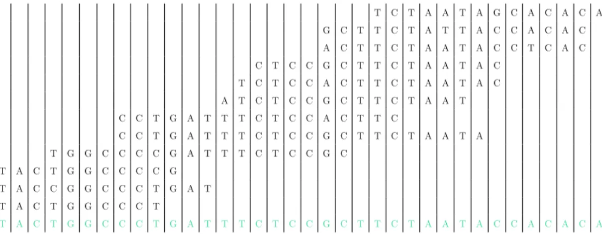
To practice a de novo assembly, DNA fragments (parts of DNA strands as sequencing machines can handle) of the target sample are collected such that they cover the genome entirely. Then, these DNA fragments are aligned against each other and merged based on overlap information to get contiguous segments (contigs). Using contigs and paired end information between reads, scaffolds are formed. Scaffolds might contain gaps next to each other.Lastly, multiple scaffolds are joined so that they form a chromosome.
Table 2.1: Larger fragments are built from small sequenced parts
T C T A A T A G C A C A C A G C T T C T A T T A C C A C A C A C T T C T A A T A C C T C A C C T C C G C T T C T A A T A C T C T C C A C T T C T A A T A C A T C T C C G C T T C T A A T C C T G A T T T C T C C A C T T C C C T G A T T T C T C C G C T T C T A A T A T G G C C C C G A T T T C T C C G C T A C T G G C C C C G T A C C G G C C C T G A T T A C T G G C C C T T A C T G G C C C T G A T T T C T C C G C T T C T A A T A C C A C A C A
On the other hand, in alignment based assembly, reads are aligned against a similar reference genome, typically from the same specie, using a read aligner that can tolerate variants up to some point. There are some other reference guided methods that use reference genome’s structure to form scaffold from contigs,
Figure 2.1: Schematic representation of the four stages of the next-generation genome assembly process (adapted from [2])
rather than using reference in the beginning of assembly procedure [22].
2.2.1
Challenges in Genome Assembly
Highly repetitive nature of human genome does not help assembly at all. Ac-cording to a study conducted in 2011, even though widely accepted claim is that about half of the human genome consists of repetitive sequences, mostly trans-posable elements; the ratio of repetitive sequences in human genome, in fact, is much higher around 66-69% [23]. Genomics regions with exact copies can not be distinguished from each other, especially if repeat length is greater than the read length. Nevertheless, single reads that cover repetitive region and non-repetitive unique sequence next to it might help to make this problem easier. Paired end reads and information about average distance between pairs together are certainly useful for assembly as well [24].
Unfortunately, repetitiveness is not the only problem about sequence assem-bly. Depending on sequencing chemistry methods, various kinds of errors, such
as deletion, insertion, substitution or other platform-specific issues, may appear during the whole amplification and sequencing processes. Average error rates are below 0.4%, 1.78% and 13% for sequencing platforms Illumina, Ion Torrent and PacBio, respectively. More importantly the number of reads that do not contain any kind of error are 76.45% for Illumina MiSeq, 15.92% for Ion Torrent and 0% for PacBio [25]. This is where a need arises for alignment tools which is capable of tolerating sequencing errors. However, imperfect error tolerance algorithms would lead to other problems such as false positive joins. This problem occurs principally in reads from polymorphic repeats, which is highly important for STR discovery.
Sequence assembly might also be affected negatively by non-uniform coverage of sample genome and non-uniform distribution of fragment lengths.
Differences inherited from two parents can be presented as another barrier for a smooth sequence assembly, although most studies so far ignore ploidy. Since STRs are polymorphic and we aim to take the diploid nature of DNA into consideration, it requires and additional effort and more detailed analysis to do to it properly.
The assembly problem we are dealing with in the scope of this thesis can be considered as local assembly, which is the assembly procedure of reads that maps to an extremely small part of the genome.
2.2.2
Assembly Methods
NGS assemblers are usually based on three paradigms: (i) constructing contigs by a greed approach, (ii) de Bruijn graph (DBG) based method that rely on a variant of k-mer graph, and (iii) overlap-layout-consensus (OLC) methods that are based on an overlap graph [24]. In the scope of this thesis, we will be focusing on two general approaches that make us of graph data structures.
2.2.2.1 De Bruijn Graphs
k-mer is a substring of length k. k-mer graph, on the other hand, is a graph data structure in which each k-mer is a node and an edge between two nodes implies they are neighbors in the genome sequence. De Bruijn Graph method is based on k-mer graphs [26].
Eulerian walk is a path on a graph that visits every edge exactly once, which does not necessarily exist for every graph. Indeed, Eulerian walk is available on a directed graph if and only if it has at most two semi-balanced nodes (indegree differs from outdegree by 1) and all other nodes are balanced. As long as each k-mer belongs to one read, de Bruijn Graph is going to have an Eulerian walk. Eulerian walk on a de Bruijn Graph gives the reconstruction of original genome sequence [3].
In order to build the de Bruijn Graph for genome assembly, all reads are first chopped into k-mers and their adjacency relation is preserved on the edges. As seen on Figure 2.2, an edge on the de Bruijn Graph corresponds to an overlap (of length k-2) between two k-1-mers. More clearly, it corresponds to a k-mer from the initial sequence [27]. In the ideal scenario, assuming sequencing data is perfect (i.e. error free k-mers with full coverage), the de Bruijn Graph built from reads would contain an Eulerian path, which is trivial to find in linear time [28]. Hence, assembly problem becomes trivial.
Perfect sequencing data is not a good assumption to make, though. There are multiple issues that affect efficiency of DBG based assemblers and require additional computation:
• Repeats: There will always be complex repeat structures in the real data, which may cause multiple Eulerian walks on the de Bruijn Graph. It is not possible to infer the correct path if there are multiple branches. There-fore, DBG assemblers typically make use of reads and mate pairs to resolve branches caused by repetitive regions.
Figure 2.2: de Bruijn graph of AAABBBA with k-mer length 3 (adapted from [3])
• Sequencing errors: Faulty reads may lead to redundant nodes in the de Bruijn Graph. Assemblers usually include a pre-processing step for reads to eliminate erroneous data or they try to eliminate graph edges that is not supported above a threshold value (number of reads).
DBG based assemblers are mostly used on the short reads. Although it does not store individual reads, it keeps the whole sequence in memory, which can be exhaustive on large genomes. The most important benefits of this approach are speed and simplicity.
2.2.2.2 Overlap-Layout-Consensus Method
OLC works similar to DBG in terms of utilizing overlap information about reads [29]. However, it uses this information in a different way.
De Bruijn Graph method is counter-intuitive. Although the goal in DNA sequencing is to achieve longer reads, DBG splits those reads into even shorter k-mers. By doing this it loses connectivity information on reads. As reads get longer, more information is lost. OLC method builds an overlap graph instead where reads are represented as nodes and overlaps as edges [26].
OLC method is a three step approach:
1. Overlaps are computed explicitly by all-against-all, pairwise read aligning. This step is based on shared mers among reads and can be tuned with k-mer size, minimum overlap length and minimum percent threshold required to identify overlap parameters [27].
2. In the layout step, the aim to merge reads into contigs. This is achieved by removing transitively-inferable edges that skip one or two edges. This is, in fact, finding a Hamilton path, which is known to be an NP-hard problem. However, there are greedy algorithms that are good approximations and often used in this step.
3. Lastly, a consensus sequence is derived from a profile of the assembled frag-ments using multiple sequence alignment (MSA). Even though it is theoret-ically possible to exploit statistical methods and weighted voting strategies to obtain the optimal MSA, there is no known efficient way to compute it [26]. That is why this phase uses progressive pairwise alignments.
In OLC method, the number of nodes kept in the graph is linearly proportional to sequencing depth. It is much less memory intensive compared to DBG. Hence, OLC fits well with the low-coverage long reads; whereas DBG is more suitable for short reads with high coverage [26].
2.3
Tandem Repeats
Tandem repeats are pieces of DNA where a pattern has multiple consecutive copies adjacent to itself. They cover more than 10% of the whole genome [30]. If the repeat unit (pattern) consists of 2 to 6 nucleotides, it can be referred as a short tandem repeat or a microsatellite.
not gained enough attention to be a permanent step in genome sequence anal-ysis pipelines. However, several approaches to call them from high throughput sequencing (HTS) data have been proposed in the recent past. Two approaches used in phase 3 data of 1000 Genomes Project (1KG) are lobSTR [11] and Re-peatSeq [12], which are released in June 2012 and January 2013 respectively [31]. lobSTR accepts raw reads as input data and only aligns the ones which fully encompass repeat region with its upstream and downstream flanking regions. Aligning all reads using other mainstream aligners is the most cumbersome part of variant calling. By not doing so, lobSTR gains a big advantage. According to their experiments, lobSTR is remarkably faster than conventional aligners; 22 times against BWA, 70 times against Novoalign, and 1000 times against BLAST [11].
Three main steps of lobSTR’s algorithm can be summarized as follows:
• Sensing is the part for (i) filtering reads such that only reads containing an STR region with its anchors are left and (ii) finding repeat unit itself. This procedure relies on a signal processing approach. Based on their reportings, they have the highest ratio of reads with non reference allele versus total informative reads.
• Alignment part is to find remaining reads’ positions on the reference genome using their anchors and provided reference STR regions.
• Finally allelotype step reports allelic configuration of region using some statistical learning approach.
The other method applied on 1KG, RepeatSeq, takes alignment files from any mainstream aligner as input and realigns them to get a higher chance for minimizing the number of mismatching bases. For each reference repeat region given, it first excludes reads that do not span across the entire repeat region, and then tries to estimate genotypes using Bayesian approach with the following features as prior information: reference length of repeat, repeat unit size and average base quality of read.
Although lobSTR and RepeatSeq have their own ways to handle aligning reads to reference genome, they both suffer from covering only STRs shorter than the read length. In fact, since they use reads that contain anchors, their size limitation is much more strict than the read length (see Chapter 4 for results).
Considering the facts that (i) some individuals or ancestries might have notably larger copy numbers than those seen in general population and (ii) having longer repeat regions might have some biologically critical consequences; limitations of these tools is important enough to mention. As an example, while most humans have 30 CGC repeats in FMRI gene, FMR1 alleles with copy numbers in between 55 and 200 are associated with neurodegeneration and ovarian insufficiency. Or alleles with more than 200 repeats associated with intellectual disability and autistic symptoms [8]. FMR1 gene is not the only one whose expansion can be correlated with abnormal phenotypes. Those cases are certainly off capabilities of lobSTR and RepeatSeq. Therefore, even if read length in sequencing machines have been increasing continuously, discovering longer STR regions is not straight-forward and definitely requires more attention.
Chapter 3
Materials and Methods
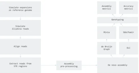
In this chapter we provide detailed descriptions of each step in our STR charac-terization pipeline, as visualized in Figure 3.1.
3.1
Overview of the Approach
According to our literature survey, there are approximately 30 assembly tools which use different algorithms and data structures to optimize their resource consumption. A non-exhaustive chronological list of sequence assembly tools in large genomes would be as ABySS, SGA, SOAPdenovo version 2, Minia, DISCO-VAR, and BCALM2 [32, 33, 34, 35, 36, 37] - from 2009 up to 2016. Each one has its own advantages over others, mostly focused on parallelization of work and advanced data structures to represent underlying assembly graph.
For example, ABySS was the first software to assembly whole human genome from short reads by distributing a de Bruijn graph across a cluster of nodes [32]. A more recent tool, Minia also uses de Bruijn graphs but reduces memory require-ments using Bloom filter, which is a space efficient hash-based data structure to check existence of an element. According to their experiments, peak memory us-age for Minia is 5.7Gb, whereas memory consumption of ABySS goes up to 336Gb
Figure 3.1: STR characterization pipeline
for de novo human genome assembly. However, this a trade-off; lower memory usage comes with consequences: execution times for the same two tools are 23h and 15h respectively. Even if they have some differences, percentage of contigs that they could align to reference with at least 95% identity only changes 0.4% between these two [36]. This conclusion applies to tools using overlap-layout-consensus based algorithms as well.
On the other hand, a recent study reveals that an OLC-based method is able to assemble a genome sequence with ten times higher N501 compared to a de
Bruijn graph approach. Besides, mean length for generated contigs is also ten times longer while the number of contigs are only one-fifth [39]. Hence, accuracy rates or the capability to assembly a genome as a whole might differ a lot.
The main aim of this work is to use sequence assembly methods for regions where we know that there is an STR, based on reference genome, and release a complete pipeline from sample’s reads to STR genotype. In the lights of infor-mation about genome assembly tools, we have selected three different assemblers to be integrated into our pipeline: SGA, Minia, and Pamir.
1The length of the smallest contig x, which makes the ratio of cumulative length of contigs
from this length x to largest contig size covers at least 50% of the bases of the assembly. An assembler with high N50 size value is obviously considered to be a high quality assembler [38].
However, since we use assemblers only on relatively short regions, we do not expect choosing a specific assembler tool to have a prominent impact on the end result as long as they use the same underlying method. Local assembly is going to even out their advantages. We will discuss this issue further in the experiments section.
3.2
Simulating Expansions on Reference Genome
In this step, we extract STR regions from reference genome and alter their copy numbers them with simulated events.
3.2.1
Tandem Repeat Regions from TRF
As opposed to other variation callers for structural variations, SNPs or indels, short tandem repeat tools require an input file that contains STR regions in the reference genome. Regions are gathered by using the same reference version with alignment step. Finding tandem repeats in a sequence is a well studied problem in different domains. For example, pattern matching in long strings in computer science is a form of technically the same problem.
Most of the tools in the field use a two-phase approach: search and filtering. In the search phase, the intuitive approach would be dividing the entire sequence into subsequences and comparing every adjacent region with each other for various period sizes. However, this brute force approach is exponential in terms of time complexity. Considering the size of whole human genome with millions of base pairs, it’s not a good solution. To avoid this problem, some tools use a heuristic or statistical approach that detects candidate repetitive loci by scanning over the sequence with a small window first, and then tries to find longer repeats [40].
In the second phase, filtering is done to identify and extract biologically sig-nificant repeats. Among multiple approaches, we have decided to use Tandem
Repeat Finder [30] for getting reference STR regions, as it has been the most popular tool used by many researchers in large projects so far.
We downloaded TRF output for chromosome 20 of GRCh37, ran with default parameters and filtered it based on our needs so that:
• Repeat matches are perfect, that is there is no change in repeat unit. • Both copy number and repeat unit length are greater than 3.
In the end, we obtained 1963 STR regions from reference genome for chromo-some 20, ready for random event simulation as the next step in the pipeline.
3.2.2
Random Homozygous/Heterozygous Event
Simula-tion
After extracting 1963 STR regions from chromosome 20, we ran multiple versions of event simulations to generate synthetically expanded STR regions. The simula-tion accepts STR regions (TRF output) and reference genome (FASTA) as input and produces two inflated sequences together with metadata about expanded regions (updated end location, new copy number, genotype, etc).
Workflow in this step for each STR region is as follows:
• Randomly chose between homozygous or heterozygous genotype • Randomly pick an expansion factor N between 1 and 30
• Identify the STR region in the reference genome • Inflate the sequence by inserting N more repeat units
If the genotype is homozygous, both alleles have the same expansion, i.e. same sequence. If it is heterozygous, one allele might be the same as reference genome
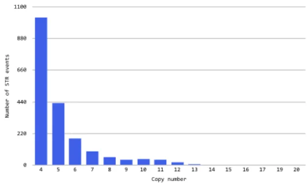
while the other one has a random expansion, or they both can have different random expansions. Number of STR events 0 220 440 660 880 1100 Copy number 4 5 6 7 8 9 10 11 12 13 14 15 16 17 19 20
Figure 3.2: STR events per copy number (reference)
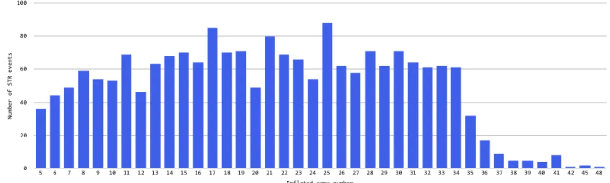
The distribution of inflated copy numbers is presented in Figure 3.2 and 3.3.
3.3
Simulation of Illumina Reads Using Mitty
It is quite common in bioinformatics studies to use synthetic reads in the pipeline mainly because either they believe there is no high quality gold standard set to compare results against or they are more keen to try out their methods on a more predictable dataset before jumping into more complicated cases with the real genome. Both reasons are applicable to our study.
Mitty is a tool that generates synthetic next-generation sequencing reads, mainly for Illumina platform [41]. It has five built in read models with changing error profiles, read lengths and fragment size distributions, which you can use out of the box to simulate reads. Besides, in the case that one of the existing models does not match your requirements, there is also an option to build an empirical model based on a provided alignment file.
The two most useful features of this software are:
Number of STR events 0 20 40 60 80 100 Inflated copy number 5 6 7 8 9 10 11 12 13 14 15 16 17 18 19 20 21 22 23 24 25 26 27 28 29 30 31 32 33 34 35 36 37 38 39 40 41 42 45 48
Figure 3.3: STR events per copy number (inflated)
allows you to work with non-corrupted versions of reads, as well.
• It has a “god aligner” module for providing the correct alignment file to eliminate errors that alignment tools might generate.
For all our simulation experiments, built in HiSeq X version 2.5 Garvan read model has been used with varying coverage depths. Some features of the model [41]:
• It has 1.92% mean error rate at first pair, whereas it is 7.46% for the second pair.
• The average fragment size distribution is 350, and it has a normal distribu-tion.
• The read length is 150bp.
3.4
Aligning Reads Using BWA-MEM [1]
Capability to generate sequences grows exponentially faster than our capacity to analyze it, which requires having efficient and accurate tools to utilize such volume of data. Usually, aligning reads to a reference genome is the initial step
of bioinformatics pipeline and it can be seen as one of the most time consuming yet essential step.
In general, sequence alignment software tools work on pipeline of three steps:
1. Indexing the reference genome or the reads (often using heuristics) 2. Identifying the exact or near exact matches
3. Performing dynamic programming alignment to tolerate more complex cases
It would be more useful to divide sequence aligners into groups based on the way they approach the indexing step of this pipeline.
The hash-based methods first identify a subset of possible locations for reads in the reference genome using common k-mers shared by both reads and reference genome through the hash tables. This step is the ”seed” part of seed-and-extend strategy. “Extend” strategy is performing more precise approaches (e.g. dynamic programming) to eliminate some of the seeds. Hash-based methods might also differ based on the fact that whether mismatches or indels are tolerated in the seed step [42].
Second group of aligners use Burrows-Wheeler Transform (BWT) based back-tracking algorithm for indexing. They align entire set of reads (not just seeds of reads) against substrings sampled from the reference genome. To be able to search for reads efficiently, they build a data structure (such as suffix trees or FM index) that contains all suffixes of the reference genome sequence. This approach efficiently solves the issue with aligning to multiple identical copies in the refer-ence region, where hash table-based approaches do not perform as well. However, keeping all suffixes of the reference genome requires massive amount of memory [42].
BWT is a reversible data compression algorithm, which is used in order to reduce the memory burden of storing all suffixes. Hence, this group of aligners
(BWA, Bowtie, SOAP2, etc.) are able to index very quickly with reasonable memory requirements [42].
In theory, our pipeline is applicable to any BAM file generated by a read aligner that supports soft-clipping. But for this study we have selected BWA-MEM because of its efficiency and comparable accuracy [1]. BWA team also suggested to use BWA-MEM in case the read length is longer than 70bp, which applies to our work.
3.5
Assembly
3.5.1
Assembly Pre-processing
Most of the established sequence alignment tools do not only report start posi-tion of reads in the genome but also provide supplementary informaposi-tion about the alignment. Supplementary information may include fields such as CIGAR (indicator of base alignment, deletion, insertion, etc.), MAPQ (mapping quality), and QUAL (query quality).
CIGAR string provides information about insertion and soft clipping events, which makes it useful for our pipeline.
Table 3.1: Alignment with attributes POS=5 and CIGAR=3M1I3M1D5M4S
Reference Position 1 2 3 4 5 6 7 8 9 10 11 12 13 14 15 16 17 18 19 20 21 Reference C C A T A C T G A A C T G A C T A A A A A
Read A C T A G A A - T G G C T G G C T
CIGAR string is a sequence of events with base lengths. Each one indicates an event such as alignment match (M), insertion to the reference (I), soft-clipping (S), deletion from the reference (D), and skipped region from the reference (N).
end portions of it is unmatched with the reference genome [43]. Aligner assigns a smaller penalty for soft-clipped regions compared to mismatching bases. This is extremely desirable for finding expansions as we do not want to miss them by penalizing too much. Hence, we make use of CIGAR strings and soft-clipping information when pre-processing data for assembly.
In general, assemblers accept FASTQ files that contain reads to assemble. To build reads data, we have applied following steps for each STR region:
• Using HTSlib [44] reads that map to the STR region were extracted. For each read, we have decided whether it is a reference supporter or not. This is based on its CIGAR string, the number of exact consecutive repeat units it has, and whether these consecutive repeats are placed at both ends of the read.
• For the STR region, if it has enough reference supporters, we have decided that at least one of the alleles has the same copy number with the reference and filtered all reference supporter reads so that we can get a better and clean assembly. Using all reads that map to the STR region would not be fair in the experiments since some STR callers use the reference copy number as a prior information to make better calls.
• Lastly, we have prepared a SAM and a FASTQ file containing reads that passed pre-processing filter.
3.5.2
SGA as the Assembler
SGA (String Graph Assembler) is one of the early adopters of string graph based approach for assembling short reads. In order to decrease memory usage, it utilizes a compressed index for set of sequence reads. Despite being one of the very firsts of its type in genome assembly, it is still widely used in many projects [33].
Each step in SGA pipeline is exposed as a different module, so that each one can be updated independently to keep up with new sequencing technologies or improved algorithms. This way, it also provides a flexibility to skip or rerun any step independently if needed.
For example, since we are dealing with very short regions, scaffolding is not necessary. Indeed, it did not give a different result than contigs in our experi-ments. That’s why we skipped the scaffolding module that uses pairs of the reads to connect contigs to each other.
Submodules we have used in the scope of this work are:
• Preprocess: It filters or trims reads with low quality or ambiguous base calls. However, for our case paired-end mode and filtering based on quality are disabled. This is because we have already applied a filtering and we wanted to be fair to all assemblers in the experiments in case they do not have this module.
• Index: The FM-Index is a data structure that allows efficient searching of a compressed representation of a text and commonly used on top of Burrows-Wheeler transform of the text. BWT compression and FM-indexing to-gether are useful especially for high coverage data. SGA uses them for indexing reads. We run indexing module twice in the pipeline, first with pre-processed raw reads and then with corrected reads.
• Correct: Having a built-in read correction bundle in an assembly software is practical. This bit can be applied to correct base calling errors using two different algorithms: (i) based on k-mer frequencies and (ii) based on inexact overlaps between reads. K-mer based correction, which is preferred in our work, is similar to what other assemblers do [33]. It basically marks a base call as trusted if that position is covered by a k-mer at least c times, where c being a parameter decided by SGA itself. For untrusted positions, it tries alternative bases so that it can replace them with a read of which all positions are trusted. If no alternative is found or there is more than
one alternative with same frequency, the read stays unchanged. We choose k for k-mers as 41 and 63 based on their suggestion for human genome [33].
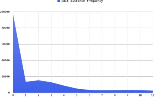
From 1963 STR regions we worked on there were 173,342 reads in total. 76,090 of these reads were corrected by SGA Correct module. Based on SGA Error Cor-rection module, only 56% of reads are error free, which is less than expected according to average error rates of Illumina platform. x-axis of Figure 3.4 shows edit distances between reads and their corrected versions; whereas y-axis repre-sents the frequencies. Most of the reads have 1, 2, or 3 mismatches, while the highest edit distance with a read and its processed version is 11. More interesting comparison as a future work might be looking at the non-STR regions to compare the error rate reported by SGA.
• Filter: This step filters reads having exact matches (including reverse com-plements) before starting to build the graph.
• Overlap and Assemble: These last two parts construct the graph using fil-tered and corrected reads and try to find a path in the graph to report as a contig. When deciding overlapping reads, the parameter that defines whether reads are neighbours in the graph or not (minimum overlap re-quired between two reads) is tuned as 70. Even if it does not apply to local assembly, their improvement on graph building, where they construct assembly graph locally around each read and merge them later instead of loading full graph, has many advantages for whole genome assembly. Based on parameters we have set, a path to be reported as a contig should at least have 90 bases across its nodes.
3.5.3
Minia as the Assembler
As opposed to modular approach of SGA, Minia is presented as a whole package. While this makes providing specific configuration for sub-steps quite complicated, it is much more straightforward to use the tool as a complete assembler.
0 20000 40000 60000 80000 100000 0 1 2 3 4 5 6 7 8 9 10 11 Edit distance frequency
Figure 3.4: Frequency of edit distance between reads and their corrected versions
As mentioned in Section 2.2.2, de Bruijn graph based assemblers are abso-lutely less time consuming compared to Overlap-Layout-Consensus graph based methods. However, speed comes with an huge memory burden. A de Bruijn graph based assembler without any additional data structure or algorithmic op-timization, requires nearly 15Gb of memory to store just the nodes alone when working on the human genome (k-mer size being 27) [35]. There have been studies to tackle memory consumption of de Bruijn graph, primarily focused on (i) enabling distributed computation on the graph to reduce memory usage per node, (ii) storing less data in the graph by omitting read locations and paired end information, (iii) greedy algorithms to compute local assemblies around related sequences [35]. Minia, on the other hand, makes use of Bloom filter to improve memory efficiency of de Bruijn graphs.
Bloom filter is a hash-based data structure that is specifically designed for checking existence of element in a set and to be space efficient. By its design, Bloom filter does not guarantee that element exists in the set even if lookup oper-ation returns true. Whilst, a false return value indicates that element is definitely not in the set. Therefore, Bloom filter may have false positives, probability of which is directly proportional to the size of the set [45]. In order to overcome false positives coming from the Bloom filter, Minia utilizes an additional data structure to keep track of critical false positive k-mers.
and searches for its neighbours in the Bloom filter. If the Bloom filter returns negative, no edge is placed in between. If it returns positive, in order to avoid false positives it performs an additional lookup to auxiliary data structure. If it confirms the positive value, an edge is placed between k-mer nodes.
Once the graph is constructed, breadth first traversal returns contigs. Minia does not provide a module that supports scaffolding using paired end information. According to the developers of Minia, optimal k-mer size is determined as 47 for chromosome 14 assembly with 100bp reads [35]. We decided k-mer size to be 63 since reads in our work are longer (150bp).
3.5.4
Pamir as the Assembler
Pamir is a software for novel insertion detection [46]. It popped into our radar because novel insertions can only be detected using de novo assembly. We have extracted custom assembly module to be able to use it as a standalone application. Pamir’s in-house assembly algorithm is based on OLC with an important tweak. It takes strand-specific information into account, which can be inferred from the mapping information. Since it knows which strand to pick, duplicate calculation for reverse complement can be avoided. That is why we thought that it would be reasonably more time efficient compared to conventional assembly methods. Experiments verified our initial view, which will be discussed further in Chapter 5.
3.6
Genotyping
Genotyping is the process of determining the genetic constitution of an individual, which has been inherited from the parents. Since human genome is diploid, we have two alleles for every part of our genome. The output of this step is going to
0 250 500 750 1000 1 2 3 4 5 6 7 8 9 10 11 12 13 14 15 SGA Minia Pamir
0 250 500 750 1000 1 2 3 4 5 6 7 8 9 10 11 12 13 14 15 SGA Minia Pamir
Figure 3.5: Produced number of contigs for homozygous and heterozygous events, respectively
be one of the following:
• Heterozygous: Each parent contributes different alleles. To call it as het-erozygous, one of the alleles must be different from the reference allele. The other one is not necessarily different than reference allele.
• Homozygous: Parents contribute the same allele, which is always different from the reference allele.
As the last step in our pipeline, we perform genotyping on the reported contigs. Ideally an assembler should produce a single contig for an homozygous event, and two contigs for an heterozygous event. Most of the time assemblers produce more contigs than the number of different alleles. Figure 3.5 reports the number of contigs produced by assembler in homozygous and heterozygous events, respec-tively. Figure 3.5 shows that all three assemblers have struggled resolving reads into the correct number of contigs while SGA performed relatively well. Pamir have always produced way too many contigs than 15, which is due to the fact that it does not apply post-processing. Minia has been more successful compared to Pamir, whilst it has failed to resolve regions that are larger than k-mer size.
In order to decide which contig is more accurate, we take sequences reported by reads into consideration. We first tried to align reads to all contigs and select
the contig with the highest mapping score using classic Smith–Waterman local alignment for each read. However, since Smith-Waterman local alignment did not scale well in terms of time complexity, we have decided to apply BWA-MEM after considering the facts explained in Section 3.4.
Upon obtaining the most supported two contigs, we infer genotype based on the following rules:
• If read support ratio of these contigs is too low, we conclude that it is an heterozygous event.
• If one of the contigs is supported by most of the reads, while the other one has a low support, we conclude that it is an homozygous event.
As a side note, depending on whether reference allele is available in the re-gion after pre-processing filter or not, copy number for one of the alleles can be obtained directly.
Chapter 4
Experimental Results
In the experiments, we wanted include a calling method that does not depend on assembly as a comparison. Based on a recent study which evaluates non-assembly methods for detecting STRs, HipSTR, lobSTR, and RepeatSeq are leading the competition [47]. Although HipSTR outperformed others in their experiments, it is designed for population data and requires high coverage to detect de novo mutations, which makes it unsuitable for our study. Hence, we included lobSTR in our experiments.
There are three experiments presented in this chapter, each focusing on a different aspect:
• First experiment is to evaluate methods based on their performance on separate genotypes.
• Second one is to analyze how sequence coverage impacts assembly based callers.
• The last experiment assesses the importance of pre-processing and including flanking regions.
4.1
Genotype Based Performance
In this experiment we have simulated events based on 1963 STR regions retrieved from TRF with a sequencing coverage 60X. Each region was inflated by a random amount of copy numbers (between 1 and 30) and randomly assigned a genotype. In all heterozygous events, alleles coming from each parent have different copy number and both of them are different from reference allele.
True positive rates1 of methods are reported as a distribution over repeat
region size (i.e. copy number times repeat unit length). In order to tolerate randomness and volatility in short spans, events are grouped into bins based on repeat region size. Each bin contains events from a range of five size values. For instance, bin-20 contains all events having a repeat region longer than or equal to 20nt and shorter than 25nt.
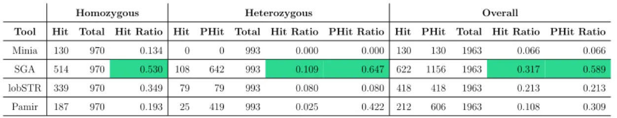
Table 4.1: True positive rates for all events
Homozygous Heterozygous Overall
Tool Hit Total Hit Ratio Hit PHit Total Hit Ratio PHit Ratio Hit PHit Total Hit Ratio PHit Ratio Minia 130 970 0.134 0 0 993 0.000 0.000 130 130 1963 0.066 0.066 SGA 514 970 0.530 108 642 993 0.109 0.647 622 1156 1963 0.317 0.589 lobSTR 339 970 0.349 79 79 993 0.080 0.080 418 418 1963 0.213 0.213 Pamir 187 970 0.193 25 419 993 0.025 0.422 212 606 1963 0.108 0.309
In distribution charts, x-axis represents bins while y-axis represents true posi-tive rate.
To report some statistics about the events:
• As presented in Table 4.1, genotype split in 1963 events is 970 homozygous to 993 heterozygous.
• Bin-115 is the largest bin containing 128 STR events (see Figure 4.4). • Shortest and longest repeat regions are composed of 20nt and 220nt,
re-spectively.
0.00 0.20 0.40 0.60 0.80 1.00 20 30 40 50 60 70 80 90 100 110 120 130 140 150 160 170 180 190 200 210 220 Minia SGA lobSTR Pamir
0 30 60 90 120 150 20 30 40 50 60 70 80 90 100 110 120 130 140 150 160 170 180 190 200 210 220 Events
Figure 4.1: (Left) True positive rates for homozygous events vs. region length and (Right) number of homozygous events vs. region length
As seen in Figure 4.1, SGA is clearly the most successful at calling homozygous STRs, followed by lobSTR. It does not only cover the widest range in terms of repeat region length but also dominates other approaches in almost every bin, which reveals that read length is not a major barrier for SGA unlike lobSTR.
Figure 4.2 and Figure 4.3 present true positive hit and partial hit rates on heterozygous events. On a heterozygous STR event, if caller is able to determine copy number for both alleles, it is considered as a hit. If it calls only one of the events, it is a partial hit. SGA is still definitely more effective at detecting at least one of the alleles correctly. However, especially in shorter repeat regions, lobSTR performs better by a large margin at calling events on both alleles. For regions longer than 65nt, there is a significant drop in lobSTR’s effectiveness.
In general, considering lobSTR’s 0.349 hit ratio in homozygous events versus 0.080 in heterozygous cases, it has a substantial disadvantage in calling heterozy-gous STRs. Minia and Pamir have underperformed in all cases (see Figure 4.4)
Table 4.2: Genotype calls an all events
Homozygous (970 events) Heterozygous (993 events)
Tool Correct Call Correct Call Ratio Correct Call Correct Call Ratio
Minia 474 0.489 560 0.564
SGA 725 0.747 517 0.521
lobSTR 359 0.370 76 0.077
0.00 0.20 0.40 0.60 0.80 1.00 20 30 40 50 60 70 80 90 100 110 120 130 140 150 160 170 180 190 200 210 220 Minia SGA lobSTR Pamir
0 30 60 90 120 150 20 30 40 50 60 70 80 90 100 110 120 130 140 150 160 170 180 190 200 210 220 Events
Figure 4.2: (Left) True positive rates for heterozygous events vs. region length and (Right) number of heterozygous events vs. region length
0.00 0.20 0.40 0.60 0.80 1.00 20 30 40 50 60 70 80 90 100 110 120 130 140 150 160 170 180 190 200 210 220 Minia SGA lobSTR Pamir
Figure 4.3: True positive rates (partial) for heterozygous events vs. region length
with similar true positive rates (0.066 and 0.108, respectively). Although all ap-proaches have at least 4-times lower rates in heterozygous STRs, Minia (and de Bruijn graph) failed to detect even a single one.
We have also examined their abilities to annotate genotype of the STR region without taking the reported copy numbers into account. Genotype annotation accuracies are presented in Table 4.2. lobSTR reported only 76 of 993 heterozy-gous events as heterozyheterozy-gous, while Pamir is the best performing with 628. On the other hand, SGA is better at annotating homozygous regions. On the ba-sis of this results, it is safe to say that assembly based methods are superior to lobSTR, which proves that discovering the existence of different alleles are easier with local assembly. To sum up, none of the methods help us genotype an STR region confidently.
0.00 0.20 0.40 0.60 0.80 1.00 20 30 40 50 60 70 80 90 100 110 120 130 140 150 160 170 180 190 200 210 220 Minia SGA lobSTR Pamir
0 30 60 90 120 150 20 30 40 50 60 70 80 90 100 110 120 130 140 150 160 170 180 190 200 210 220 Events
Figure 4.4: (Left) True positive rates for all events vs. region length and (Right) number of events vs. region length
4.2
Coverage Tests
There are 1963 simulated STR regions with a 966/997 split between geno-types (homozygous/heterozygous) in this experiment. However, for heterozygous events, this time one of the parents has the same allele with the reference region. In this group of runs, we aimed to assess the impact of sequence coverage on assembly based callers. We simulated sequence data from the altered genome with multiple sequence haploid coverage, at 40X, 60X, and 80X. True positive rates for each caller with different coverages are reported in Figure 4.5, 4.6, 4.7, and 4.8. 0.00 0.20 0.40 0.60 0.80 1.00 20 30 40 50 60 70 80 90 100 110 120 130 140 150 160 170 180 190 200 210 220 80x 60x 40x
Figure 4.5: True positive rates of SGA with different coverages vs. region length
0.00 0.20 0.40 0.60 0.80 1.00 20 30 40 50 60 70 80 90 100 110 120 130 140 150 160 170 180 190 200 210 220 80x 60x 40x
Figure 4.6: True positive rates of lobSTR with different coverages vs. region length 0.00 0.20 0.40 0.60 0.80 1.00 20 30 40 50 60 70 80 90 100 110 120 130 140 150 160 170 180 190 200 210 220 80x 60x 40x
Figure 4.7: True positive rates of Minia with different coverages vs. region length
the percentage of increase in recall is different between 40X to 60X and 60X to 80X. It slows down, which suggests that we are close to a saturation coverage value. For example, SGA were able to call 1.39 times as more events with 60X coverage when compared to 40X coverage; whereas the rate grows 1.12 times when coverage went up from 60X to 80X.
Reported in Table 4.3, SGA and lobSTR handle low coverage relatively well. Pamir hits jump 300% percent with 60X coverage in comparison with 40X. Having higher coverage data is more crucial for assembly based methods. Hence lobSTR’s efficiency is not dramatically affected by the coverage.
0.00 0.20 0.40 0.60 0.80 1.00 20 30 40 50 60 70 80 90 100 110 120 130 140 150 160 170 180 190 200 210 220 80x 60x 40x
Figure 4.8: True positive rates of Pamir with different coverages vs. region length
De Bruijn graph fails once again. The range of region lengths that Minia is able to call is the smallest among all callers. It could not detect any STR region that is longer than 70nt.
Hit rate lines for Pamir at 60X and 80X coverage almost overlap in each bin, which signals that it does not depend on high coverage data.
Table 4.3: True positive rates for 40X, 60X, and 80X coverage
40X 60X 80X
Tool Hit Hit Ratio Hit Hit Ratio Hit Hit Ratio
Minia 142 0.072 194 0.099 224 0.114
SGA 568 0.290 793 0.404 892 0.455
lobSTR 487 0.248 589 0.300 615 0.313
Pamir 92 0.047 289 0.147 331 0.169
As the repeat regions get longer, it becomes harder to assemble them. Besides, higher coverage values increase the variation. Considering these two facts, as seen in Figure 4.5, for STR regions longer than 100nt, SGA performs worse with high coverage data (80X).
0.00 0.20 0.40 0.60 0.80 1.00 20 30 40 50 60 70 80 90 100 110 120 130 140 150 160 170 180 190 200 210 220 SGA Preprocessed SGA Flanking SGA
Figure 4.9: True positive rates of SGA with different setups vs. region length
4.3
Assembly Pre-processing and Flanking
Re-gions
In this experiment, we have tested a single tool with a different pipeline and a configuration. SGA was clearly the best caller in all runs. We wanted to assess the possibility of increasing its sensitivity even more. The same set of STR regions is inputted to:
• An SGA pipeline with pre-processing, same as previous experiments. Pre-processing includes, as explained in Section assembly preprocess, check-ing reference supporter reads for STR regions and assigncheck-ing reference copy number to at least one of the alleles and filtering out these reads from the assembly.
• A regular SGA pipeline without pre-processing step.
• A regular SGA pipeline with flanking regions included from both ends of the STR region.
True positive rates are reported in Figure 4.9. First of all, it is certain that in-cluding flanking regions didn’t help STR variant calling at all and indeed it made it worse. This is probably caused by STR regions becoming more complicated as
they get longer. Reads from STR regions themselves cover the flanking regions enough to identify the region. Pre-processed assembly, on the other hand, gave SGA’s performance a slight boost in every bin.
Chapter 5
Discussions
We addressed the problem of short tandem repeats not being a part of large scale projects due to characterization limits. We proposed an end-to-end solution for STR characterization using local assembly that is suitable for WGS pipelines.
We concluded that String Graph Assembler is better than both other assembly based tools and state-of-art STR callers in estimating repeat numbers. However, since it uses a relatively costly OLC approach, it is lagging far behind the rest of the methods in terms of time complexity. lobSTR and Pamir have comparable runtimes and are considerably faster than Minia. At this state, we greatly value correct variant detection over runtime complexity.
State-of-art STR callers that do not make use of local assembly, expect STR regions to be covered with flanking regions. All experiments supported that for reads of length 150 base pairs, discoverable STR region is up to 70 base pairs for them. This may be overcame with the help of new long-read sequencing meth-ods, though. However, OLC based assembly methods will definitely benefit from longer reads, more than other STR callers or de Bruijn Graph based approaches [26].
We observed from coverage tests that higher coverage boosts the sensitivity of every approach. However, it does not linearly improve the number of STR regions
![Figure 2.1: Schematic representation of the four stages of the next-generation genome assembly process (adapted from [2])](https://thumb-eu.123doks.com/thumbv2/9libnet/5627784.111624/24.918.266.698.187.493/figure-schematic-representation-stages-generation-assembly-process-adapted.webp)
![Figure 2.2: de Bruijn graph of AAABBBA with k-mer length 3 (adapted from [3])](https://thumb-eu.123doks.com/thumbv2/9libnet/5627784.111624/27.918.334.603.205.370/figure-bruijn-graph-aaabbba-k-mer-length-adapted.webp)