Graded-index fibers, Wigner-distribution functions, and the fractional Fourier transform

Graded-index fibers, Wigner-distribution

functions, and the fractional Fourier transform

David Mendlovic, Haldun M. Ozaktas, and Adolf W. Lohmann

Two definitions of a fractional Fourier transform have been proposed previously. One is based on the propagation of a wave field through a graded-index medium, and the other is based on rotating a function's Wigner distribution. It is shown that both definitions are equivalent. An important result of this equivalency is that the Wigner distribution of a wave field rotates as the wave field propagates through a quadratic graded-index medium. The relation with ray-optics phase space is discussed.

Key words: Fourier optics, optical information processing, fractional Fourier transforms,

Wigner-distribution functions, graded-index media, spatial filtering.

1. Introduction

Recently, two distinct definitions of the fractional Fourier transform have been given. In the first onel-3 the fractional Fourier transform was defined physically, based on propagation in quadratic graded-index media (GRIN media). The ath fractional

Fou-rier transform of a function was defined as follows:

Let the original function be input from one side of a quadratic GRIN medium, at z = 0. Then, the light distribution observed at the plane z = zo corresponds to the a equal to the (zo/L)th fractional Fourier transform of the input fraction, where L - ('rr/2)

(nl/n2)1/2 is a characteristic distance. The a equal to the first Fourier transform, observed at zo = L, corresponds to the ordinary Fourier transform, by design.

The second definition is based on the Wigner-distribution function4 (WDF). Here one calculates the fractional Fourier transform by finding the WDF of the input image, rotating it by an angle a = a'r/2, and performing the inverse Wigner transform.

Both definitions fulfill two natural postulates: (i) The a equal to the first Fourier transform corre-sponds to the ordinary Fourier transform. (ii) The fractional operator is additive, i.e., the ath transform

D. Mendlovic is with the Faculty of Engineering, Tel-Aviv University, Tel-Aviv 69978, Israel. H. M. Ozaktas is with the Department of Electrical Engineering, Bilkent University, Bilkent, Ankara 06533, Turkey. A. W. Lohmann is with the Angewandte

Optik, Erlangen University, Erlangen 8520, Germany.

Received 8 March 1993; revised manuscript received 22 Novem-ber 1993.

0003-6935/94/266188-06$06.00/0. o 1994 Optical Society of America.

of the bth transform is equal to the (a + b)th trans-form.

In this study we show that both definitions of the fractional Fourier transform are equivalent. The fact that two distinct definitions turn out to be identical supports the claim as to the naturalness and intrinsicalness of the definitions. To quote Minsky, "Proof of the equivalence of two or more definitions always has a compelling effect when the definitions arise from different experiences and motivations."5

We also arrive at the result that the effect of propagation through GRIN media can be described as

a rotation of the Wigner distribution of the input

function. Thus this study answers two questions: (1) How does the Wigner distribution of an input function change while propagating through a GRIN medium?

(2) Are the two fractional-Fourier-transform

defi-nitions fully equivalent?

In the following we show that the answer of the first question is simply that the Wigner distribution rotates uniformly with propagation distance. This answer leads to the conclusion that both fractional-Fourier-transform definitions are equivalent. Sec-tion 2 gives some mathematical details about the WDF. Sections 3 and 4 describe the two fractional-Fourier-transform definitions, and Section 5 gives the mathematical proof that both definitions are fully equivalent. Section 6 is a discussion and conclusion. The analyses presented in this paper are for one-dimensional (1-D) input functions, for notational convenience. However, all results can be extended trivially to higher dimensions, as is shown in Ref. 4.

2. About the Wigner-Distribution Function

The Wigner-distribution function6 _{(WDF) is a joint} space-frequency (or time-frequency) representation of a signal. It describes the signal completely, display-ing time and frequency information simultaneously. Applications of the WDF can be found in optics7 8 _and in the representation of speech.9 _{The WDF of a 1-D} signal f(x) can be defined as

W(x, v) = f(x + x'/2)f*(x - x'/2)exp(-2'rrivx')dx'.

(1) Using the conventional Fourier-transform operation, f(v) =

9'{f(x)}

=

f

f(x)exp(-2 rrivx)dx,

(2)

we can write an equivalent form of the WDF defini-tion as

W(x, v) =

f

f(v + v/2)f*(v - v'/2)exp(2,rriv'x)dv'. (3) Properties of the WDF can be found in Refs. 4 and 8. Here we mention three of them. First is the effect of free-space propagation in the z direction on the WDF. It was shown4 _{that such propagation} causes the WDF to be sheared in the x direction. The second is the effect of passage through a thin lens. This causes the WDF to be sheared in the v direction. The third concerns the relation between the WDF of an object and the WDF of the conven-tional Fourier transform of the same object. From Eqs. (1) and Eq. (3) one can notice that we get a r/2 rotation of the WDF. Another way to see this is to combine the effects of free-space propagation and passage through a thin lens in the form of a 2f optical Fourier-transforming setup. First, we may perform the x shearing associated with free-space propagation along a distance f, then the v shearing associated with passage through a lens with focal length f, and finally another x shearing associated with another free-space propagation along a distance f. The final result is a rotation by ,r/2 of the original VDF. For a detailed discussion of these consecutive operations with

illus-trated examples, see Ref. 4.

Consistent with our two postulates, we suggested1_-3 defining the fractional Fourier transform as the change of the field caused by propagation along a quadratic GRIN medium by a length proportional to a. Such a medium has a refractive-index profile

given by1 0

n2(x) = n2[1 - (n2/n )x2], (4)

where n and n2 are the GRIN-medium parameters and x is the 1-D coordinate. The eigenmodes of quadratic GRIN media are the Hermite-Gaussian (HG) functions, which form an orthogonal and com-plete basis set. The mth member of this set is expressed as

Pm(x)

= Hm(Q)exp(- 2)

(5)

where Hm is a Hermite polynomial of order m and is a constant that is connected with the GRIN-medium parameters. An extension to two lateral coordinates x andy is straightforward, with Pm(X)Tn(y) as elemen-tary functions. The lower-order HG polynomials are

Ho(x) = 1, H1(x) = 2x,

H2(x) = 4X2 -

2.

(6)

For a given wavelength X each HG mode propagates through the GRIN medium with a different group velocity and thus a different propagation constant,

k[l

-

2

(n2)1/2( + 1)]1/2

k

(1/2(

-

+

ni

2

(m2)

with k = 2r/X. Any function f (x) can in terms of the HG basis set as

f(x) = E Am.im(x), m (7) be expressed (8) with Am = f(x)"Im(x)/hmdX,

3. Fractional Fourier Transforms: Graded-index Media Definition

In this section the GRIN definition of the fractional Fourier transform is given. The reader can find more details in Refs. 1-3. The ath Fourier trans-form of a function f(x) is denoted as a{f(x)} As was mentioned in the introduction, we require that our definition satisfy two basic postulates. First, 5'f should be the usual Fourier transform. Our

second postulate requires that gra{bf

= a+bf.

(9)

where hm = 2m!,Fer/l/2.

Now, the fractional Fourier transform of f(x) of order a is defined as .Fa{f(x) =

I

Am1Im(x)exp(i$maL) m =

I AmPm(x)exp

i

k - (- )(m + 1 \ V

2)aL .

(10)

L = (r/2)(nj/n 2)1/2 is the GRIN length that results in the conventional Fourier transform. It was shown1 that the above two postulates are satisfied by this definition. In the same reference we also dis-cussed and proved some of the properties of fractional Fourier transforms, such as linearity, self-imaging parameters, and intensity shift variance/invariance (as with the common Fourier transform), and we generalized to complex values of the order a (which can be physically realized by attenuating or amplify-ing media).

4. Fractional Fourier Transforms: Wigner-Distribution-Function Definition

In Ref. 4 the fractional-Fourier-transform operation

is defined as a rotation of the WDF by an angle at =

arT/2. It is shown in this reference that the two postulates of Section 3 are again fulfilled. It is relevant to point out that the WDF of a 1-D function is a two-dimensional function, and the rotation inter-pretation is clear. In Ref. 4 the same rotation

strat-egy was generalized for two-dimensional signals, i.e.,

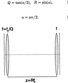
images whose WDF's are four-dimensional distribu-tions. Since any rotation can be performed as three shearing operations (x, v, and x shearings or v, x, and v shearings), it was suggested4 that the system of Fig. 1 be used to perform the fractional Fourier transform with optical means. The first lens performs the first shearing, the propagation through free space is equiva-lent to the second shearing, and the second lens is for the third shearing. It was suggested that two param-eters be used, Q and R (see Fig. 1), with

f = f1

/Q,

z = f1R, (11)

where fi is an arbitrary length, f is the lenses' focal length, and z is the distance between the lenses. For a fractional-Fourier-transform order, a, Q and R

should be chosen as

Q = tan(ua/2), R = sin(a), (12)

5. Equivalence Proof

In this section we prove that both fractional-Fourier-transform definitions are equivalent. The strategy of the following proof is to calculate the action of the optical configuration of Fig. 1 and to show that it is equivalent to propagation through a GRIN medium of a certain length. In this section the operator 7 denotes the WDF-based fractional-Fourier-transform operator. Therefore for the WDF fractional-Fourier-transform definition, because at this moment we cannot be sure whether it is the same operation as Y we rename it temporarily as ' instead of 7 and the

final result is that . =

According to the WDF fractional-Fourier-trans-form definition, by analyzing the optical configura-tion of Fig. 1, we can write

ga[f(x)] = cl exp[-ir(Q

1)

X]

Jf

x)

x exp - iw(Q - R)

x2]

x exp(-i2w dxod (14)

Cl is constant. f (xo) can be written as a superposi-tion of the HG funcsuperposi-tion set [see Eq. (8)]:

(15)

f(xo) = A.T(x),

n

where the An are calculated by use of Eq. (9). Let us substitute Eq. (15) into Eq. (14) while using T = Q

-1/R:

g'af(x) = Cl

exp(-iwrT

A

f

I

AnIn(XO) xexp(-irT Of - i27 A dxo

with (13)

f

r yi = AnaPn(X).

First, we calculate

gaqPn(x)

using mathematical

induction. We start by hypothesizing that, consis-tent with the propagation of the eigenmodes of GRIN media,

, Tn(X) = C2exp[i(n +

1)+c]I'(x)

In this expression, C2 and Xc are constants. This induction hypothesis is shown in hold for n = 0 and n = 1. Then is shown that its truth for n -

1

and n implies its truth for n + 1. This ensures that it is true for all n. First, we check the validity of the

hypothesis for n = 0. The zero-order HG function is

z=R

Fig. 1. Setup for performing a two-dimensional fractional Fourier transform according to the WDF definition.

6190 APPLIED OPTICS / Vol. 33, No. 26 / 10 September 1994

a

=

arr/2.

f=f

IQ

(16) (17) (18) :I '.I t X 2 IYO(x = exp _ W2)

From Eq. (14) one gets gat(x) =

C

₁

exp(-iTrT

A)

xf

exp(-

i'rT X2 - i2rr

dxo-Xf1 Xf 1R/dxo1

(19)

Using the known relation11

exp(-p

2

_x

2

_{+ qx)dx = p}

_exp(

q2

J

Il-ac

~

~

P p~p2 We assume

arg(C

2

)

=

-arg[( L

)

+2'

r Tr =ag1 .T 2 (O2 Xfi (25)

From Eqs. (17) and (24) one can notice that these choices agree for the special case of n = 0.

Now for the n = 1 HG order,

(20)

₂

_{2'x e x2}

1(x)

expt

-

/

(26)

Using a relation similar to Eq. (20) we can prove that

,'all(X)

=

C

2

exp(i2.)PV

1

(x),

(21) we get ak(X) = C₁ exp(-irrT Xf) _ _ _

,

)

1

X A ex(~ X2f2R2)( 1 r2)(2 1 f

/

I2 A2f2 (27)

exactly following Eq. (17).

So far we have demonstrated that Eq. (17) holds for the n = 0 and n = 1 cases. Let us now assume that Eq. (17) holds for n - 1 and prove it for n + 1:

a' an+(x) = C2exp[i(n + 2)'k1'Vn+1(X), where

_

_

_-

=

,

'Pl()= Hn11~ ex -(28) IT 1/2

x 1

T

- + Tr f

(22)

In order to adjust the last equation to the form of Eq.

(17), we choose w so as to satisfy

x2flR2

° A + T2R2 = 1 (23)

Now Eq. (22) looks the same as

g apo(X) =

C, exp(-irrT

+

Xf1 x2 x2

irT T--

_Xf, (I)/ Tr 1/2 X 1 Tl

-+

ir v/

C f'

(~

1

ir T

)]1/2C1jo(x). (24) One can notice that the field distribution of Eq. (24) is exactly the same as that of Eq. (18). As for the coefficients C1and C2, we need not demonstrate their equality explicitly since this is required anyway by the conservation of energy. The important parameters are the argument of C2and

4c

appearing in Eq. (17).

(29)

Substituting the last equation into Eq. (14), one gets gflayn+1(X) =

C, exp(-i'r

-)

JHn+i( )

(X Tx XXo X exp 0- Vir 0- i2'rr -fRdxo.

( W2 Xf, AfiR)

(30)

A known property of the Hermite polynomials is12 Hn+,(x) = 2xHn(x) - 2nHn-(x).

On the basis of this property we get

ga'yn+l(X) =

Gl(x) +

G2(X), with Gl(x) = Co exp(-irr T / 2

X

exp

-

, -

L,7r

k2

(31) (32)

f2xH(

)

1 2 aX) Txo xx₀ i2iT Idxo, X Xf1R

G

2

(x)

=

C

1

exp(-iw

A)

2

f

(-2n)HX

1

(-

)

_Xo Tx2 xx -- 0--i X i d 0°

X ep W - 1Ax f,

i2rXf

1

R d

(33)

10 September 1994 / Vol. 33, No. 26 / APPLIED OPTICS 6191 with 1 irrT

p

2 ₌

₊

_'

i2rrx

q

=-XfiR I ,ztlwl+

The induction assumption for n - 1 leads to

Gl(x)

= C

2

(-2n)Hn-i(

L)

exp(

-

(- )exp(in(C).

(34)

Now for G2(x), in Eq. (33) we can recognize a first-order Fourier-transform integral; thus

G2(x) = C1 exp(-iTr Tx2

7

f)

or

'aP+,(x)

= exp[i(n

+ 2)4C]C

2

exp(-

)

x

2x4Hn44)

_ 2nHn-,(

)]

(41)

With Eq. (31) one gets

I2

V

V

2

2I

X

x0~ TX

0

X

5

xHny

- ,exp

-

2

-i ft

(35)

A well-known property of the conventional Fourier

transform is

d

ST{xg(x)} = j- v 5{g(x)}. (36)

With the relation v = x/(f ), the use of the Eq. (36), and the induction assumption for n, Eq. (35) becomes

aTnll(X) = C2exp[i(n + 2)cC]Yn+1(x). (42)

Since Eqs. (28) and (42) are exactly the same, the proof based on the induction technique is complete,

and we can conclude that =

So far we have derived the phase coefficient at the output of the system shown in Fig. 1 when a single HG order is presented as the input. The result is shown in Eq. (17). Let us now compare this result with the GRIN-media definition of the fractional Fourier transform. For an input function f(x) the output of the configuration shown in Fig. 1 is

IC2Hn(

Q)exp(-

)

x exp (iTr - )exp[i(n +

1)4+c]}-Performing the differentiation d/dx and using'3

d dx Hn(x) = 2nHn-,(x), we get 2/ Xf, G2(X) = i j- exp[i(n + 1)+C]C2

* 2 xH2 -exp

-

k~

-½2

Xf (Vx ( x2 1

x

2nHnj-)exp - 2) * (39)

Now, Eq. (39) is substituted into Eq. (32). Using

the explicit expression of (ct [see Eq. (25)], we get

a'n11(X) = - i 2 exp[i(n +

1)-k]C

2 exPk--)

X

|

2xexp

)

4H0

)

+ -n-l( V ) (( - Ift (40

.9af(x) =

IX

An

exp[i(n +

1)4c]J'(x)-n

(43)

From Eq. (23) and the relation T = Q - 1/R it can be (37) proved that

exp(i4C) = cos(+) - i sin(+) = exp(-i-), (44)

where

4

= aIr/2. It can be seen that the GRIN (38) fractional-Fourier-transform definition, Eq. (10), has

exactly the same structure as Eq. (17) with

(45)

thus the two definitions are equivalent.

6. Discussion and Conclusion

In this section we highlight certain consequences of this equivalence. First, this implies that we have two equivalent ways of optically performing the frac-tional-Fourier-transform operation: we can use ei-ther a GRIN medium or the bulk system of Fig. 1. The GRIN-medium-based system can be considered to be more compact; however, available GRIN media

have a limited space-bandwidth product.

Another implication of this equivalence is the fact that propagation through quadratic GRIN media results in a rotation of the Wigner-distribution func-tion. This is because the bulk-optics system of Fig. 1 is fully equivalent to a GRIN medium of length aL. Until now, GRIN media have been handled mostly as ray-optics elements, mainly'0 because of the lack of simple interpretations of its effect on the wave func-tion of light passing through it. With the Wigner-distribution function we have a powerful tool for 6192 APPLIED OPTICS / Vol. 33, No. 26 / 10 September 1994

28i-- Tx 2 d

G

2

(x)

= -

exp - is

A1 dx

n2 1/2 7r

k = - - a = -a - = -(;

analyzing and designing systems with GRIN-media

devices.

Additional insight into the rotation of the Wigner distribution can be gained by examination of the ray-optics analog of Wigner space, which is a particu-lar type of phase space. We refer to the ray-optics analog of the Wigner space as the ray-optics phase space. Let a particular paraxial ray be characterized by its radial distance r and slope s, both with respect to the optical axis at a particular axial position z. Then, the effect of passing through any optical system on this ray can be described by a movement in r-s space, which is our ray-optics phase space. For instance, free-space propagation corresponds to a horizontal displacement, whereas focusing by a lens corresponds to a vertical displacement. This ray-optics phase space is analogous to Wigner space because of the correspondence between spatial

fre-quency and the angle made with the optical axis. Let us now consider a bundle of rays with a uniform spread of r and s (represented by a rectangular region in r-s space) and consider how this ray bundle is transformed as it passes through a quadratic GRIN medium. It is known that r and s obey the following

equations in such media0:

r(z + Az) = r(z)cos(ITAz/2L) - s(z)sin(7rAz/2L),

s(z + Az) = r(z)sin(iTrAz/2L) + s(z)cos(rAz/2L),

(46)

from which we can conclude that the region represent-ing any given bundle of rays in phase space is rotated uniformly as we go from z = 0 to z = L. Thus, just as the Wigner distribution does, the ray-optics phase-space distribution also rotates uniformly upon propa-gation through GRIN media.

In conclusion, propagation through quadratic GRIN media corresponds to rotation of the phase-space distributions. We have shown that this is true for two specific phase-space representations: the Wigner representation and the ray-optics phase-space repre-sentation.'

We make a final remark about the applicability: the fractional Fourier transform is a generalization of

the standard Fourier transform. The standard

Fou-rier transform is heavily involved in optical applica-tions, as the term Fourier optics implies. Hence it seems reasonable to expect optical applications when the new transform penetrates optics. Several direc-tions are suggested in Ref. 2.

We dedicate this paper to the friendship of the German, Israeli, and Turkish peoples.

References

1. D. Mendlovic and H. M. Ozaktas, "Fractional Fourier trans-forms and their optical implementation: I," J. Opt. Soc. Am. A 10, 1875-1881 (1993).

2. H. M. Ozaktas and D. Mendlovic, "Fractional Fourier trans-forms and their optical implementation: II," J. Opt. Soc. Am. A 10, 2522-2531 (1993).

3. H. M. Ozaktas and D. Mendlovic, "Fourier transforms of fractional orders and their optical interpretation," Opt. Com-mun. 101, 163-169 (1993).

4. A. W. Lohmann, "Image rotation, Wigner rotation, and the fractional Fourier transform," J. Opt. Soc. Am. A 10, 2181-2186 (1993).

5. M. Minsky, Computation, Finite and Infinite Machines (Pren-tice-Hall, Englewood Cliffs, N.J., 1967), p. 111.

6. E. Wigner, "On the quantum correction for thermodynamics equilibrium," Phys. Rev. 40, 749-759 (1932).

7. M. J. Bastiaans, "Wigner distribution function and its applica-tion to first-order optics," J. Opt. Soc. Am. 69, 1710-1716 (1979); "The Wigner distribution function applied to optical signals and systems," Opt. Commun. 25, 26-30 (1978). 8. K. H. Brenner and A. W. Lohmann, "Wigner distribution

function display of complex 1-D signals," Opt. Commun. 42, 310-314 (1982).

9. H. 0. Bartelt, K. H. Brenner, and A. W. Lohmann, "The Wigner distribution function and its optical production," Opt.

Commun. 32, 32-38 (1980).

10. A. Yariv, Optical Electronics, 3rd ed. (Holt, New York, 1985). 11. I. S. Gradshteyn and I. M. Ryzhik, Table of Integrals, Series

and Products (Academic, New York, 1980).

12. B. E. A. Saleh and M. C. Teich, Fundamental of Photonics

(Wiley, New York, 1991), p. 102, Eq. (3.3.5).

13. M. Abramovitz and I. A. Stegun, Handbook of Mathematical

Functions (Dover, New York, 1970), Eq. (22.8.7).