Simulation of a flowing snow avalanche using molecular dynamics

c

⃝ T¨UB˙ITAK

doi:10.3906/elk-1206-101 h t t p : / / j o u r n a l s . t u b i t a k . g o v . t r / e l e k t r i k /

Research Article

Simulation of a flowing snow avalanche using molecular dynamics

Department of Computer Engineering, Faculty of Engineering, Bilkent University, Ankara, Turkey

Received: 24.06.2012 • Accepted: 05.03.2013 • Published Online: 07.11.2014 • Printed: 28.11.2014

Abstract: This paper presents an approach for the modeling and simulation of a flowing snow avalanche, which is formed of dry and liquefied snow that slides down a slope, using molecular dynamics and the discrete element method. A particle system is utilized as a base method for the simulation and marching cubes with real-time shaders are employed for rendering. A uniform grid-based neighbor search algorithm is used for collision detection for interparticle and particle-terrain interactions. A mass-spring model of the collision resolution is employed to mimic the compressibility of the snow and particle attraction forces are put into use between the particles and terrain surface. In order to achieve greater performance, general purpose GPU language and multithreaded programming are utilized for collision detection and resolution. The results are displayed with different combinations of rendering methods for the realistic representation of the flowing avalanche.

Key words: Flowing avalanche simulation, snow, discrete element method, particle system, CUDA

1. Introduction

Research on the visual simulation of natural phenomena has continually advanced to generate realistic scenes of nature for both scientific and entertainment purposes. To help achieve realistic scenes, knowledge in physics and mathematics has provided an outstanding establishment to create simulations that pertain to nature’s laws. Combined with computational mathematics and advanced hardware acceleration possibilities, the research has brought numerous methods, such as particle systems [1] or grid-based systems [2], to define the base material of a natural event, such as the motion of flowing water. While much exemplary work has emerged about nature’s most common happenings, avalanching of snow has rarely been the subject to be simulated as a whole. This paper will describe a physically based method to simulate a common type of snow avalanche, defined as a flowing snow avalanche (Figure 1).

To build up a visually pleasing snow avalanche scene, 2 challenges arise. First, a fitting simulation model for avalanches that can take its physical attributes into account must be found. Next, a rendering method for the snow particles should be developed. Even though the visual simulation of snow avalanching has rarely been investigated, much work related to granular or liquid flows exists in the computer graphics literature. Thus, on one hand, the literature has visual qualification-oriented models for granular avalanches that use physically based particles and complex rendering algorithms. On the other hand, we have hazard mitigation-oriented avalanche simulations, be they statistical or deterministic (physical) models. Those solutions alone would not directly apply to a visual snow avalanche simulation. However, a combination of these methods could be useful in creating a snow avalanche scene. For instance, a dry and icy flowing snow avalanche might behave like ∗_{Correspondence: ozguc@bilkent.edu.tr}

granular material running down a slope. Thus, using molecular dynamics (MD) [3] might be a better match. In contrast, a slushy wet flowing snow avalanche may be simulated using smoothed-particle hydrodynamics (SPH) [4], because the unleashed snow’s behavior is likely that of a fluid. The examples of the application of such methods for the simulation of granular materials and snow avalanching will be described in the following sections.

Figure 1. Flowing avalanche set loose on a mountainous terrain.

2. Overview of the related methods

2.1. Snow avalanche models in the literature

There are 2 main types of approaches to model avalanches: statistical and deterministic (physical) modeling. Due to the complexity and dangerous nature of avalanches, the objectives of modeling approaches converge around hazard mitigation. Statistical modeling incurs predictions via analyzing past avalanche boundaries and extensions, so it is more focused on hazard mitigation. Adversely, deterministic modeling conveys a quantitative approach that deciphers the avalanche motion characteristics, and can be useful for both visual simulation and risk management [5]. The well-known deterministic models that are presented in the literature involve simple models that characterize avalanche motion as a sliding mass that is subject to a friction force. For instance, the Voellmy–Salm–Gubler model suggests that this friction force varies according to the avalanche mass, flow depth, path inclination, and 2 friction coefficients, which can be listed as internal and external frictional factors. The internal friction coefficient depends on the fluidity of the snow and thus to the avalanche mass, whereas the external friction force depends a lot on the path that the avalanche takes [6].

Despite there being so many publications motivated around hazard mitigation, be they deterministic or statistical [7–11], there is much less research done for a visual simulation of a snow avalanche. To our knowledge, there are 3 publications that are directly related to visually simulated snow avalanching. Chronologically, the first is Alan Kapler’s CG work for the movie “xXx” (2002), which had a mixed-motion avalanche simulation. This work was done via Houdini’s particle system with much event scripting to make the visual effects look realistic [12]. The second is again a visual effects work done for a movie called “Mummy 3” (2008). It included a mixed-motion avalanche that had finer detail of the snow packs [13]. Both of these effects underwent much

make-up for rendering them into the movie scenes. Finally, Tsuda et al. contributed a recent scientific publication that models a mixed-motion avalanche in a layered approach [14]. In this work, flowing and airborne avalanche motions were defined as dense-flow and suspension layers, and they were simulated using SPH [15,16] and a grid-based approach [17].

2.2. Molecular dynamics

The MD method was originally intended for simulating numerous discrete materials, such as molecular com-pounds or sand grains. It has a simple representation of the particle system, collision resolution, and contact generation (detection) algorithms for the granular material. The significant variables in the system are the mass, contact data, restitution, and shear friction values. Each particle may be assigned a different mass according to their sizes and they will be fixed if there is no fracture involved. Contact data are divided into 3 main parts: contact point, contact normal forces, and tangential forces. Contact normal forces involve linear or nonlinear stiffness and restitution-related calculations, whereas tangential forces incur shear friction forces, which slow down movement in the tangent direction. These forces are crucial for simulating the behavior of granular ma-terial. However, they may be insufficient to display common behavior, such as stick and slip, without necessary formal modifications.

A good example of the application of the MD method is Bell et al.’s [18] work, which provides a solution for the simulation of granular materials such as sand. With this method, the avalanching of sand can be simulated without losing the fine details of a granular flow.

2.3. Smoothed-particle hydrodynamics

Although not directly related with the work done in this paper, SPH is a valid method to be used to simulate flowing avalanches. This is due to the liquefied nature of melted snow, which lies in the core of a flowing avalanche. As in MD, the representation of a flowing mass is handled with a particle system. The decisive variables in the system are mass, density, viscosity, and pressure. In most cases, mass is divided equally among the particles. Expectedly, the density and pressure constantly change around each particle’s circumference.

Simulation of a flowing liquid may not suffice to imitate the behavior of flowing snow. Some of the methods used in recent applications of SPH may be useful in addressing these differences in order to simulate flowing snow. Adams et al. used an adaptively sampled particle system to focus on simulating fluid behavior on complex geometries [19].

2.4. Parallelization of physical simulation of particles

Particle systems, by nature, are highly parallelizable. This is due to the fact that each particle can be integrated (processed) independent from another. Intel’s Ticker Tape [20] multithreaded particle system on a central processing unit (CPU) provides a good example of parallelization. The integration work of the particle system is shared among the physical processor cores, allowing multiple particles to be integrated at the same instant. They achieve 2 times higher performance while scaling from 2 to 4 physical cores, albeit with no mentioning of interparticle collision detection.

Kruger et al. used a graphics processing unit (GPU) texture memory to dump the particle position data and process them in place, in order to integrate a large sum of particles. Using fragment shaders to build and process particle data, they improved the integrator performances to be up to 110 times faster [21].

Hegeman et al. built a dynamic quad-tree structure on a GPU to facilitate the interparticle neighbor searching in order to speed up the collision processing. They achieved up to 2 times higher performance gain compared to CPU implementation [22].

Harada et al. achieved up to 28 times faster performance for a SPH simulation by exploiting a GPU’s parallelized structure. All of the system data are located on the GPU and coding is handled on a vertex and fragment shaders on top of C++/OpenGL [23].

Another example of a parallelized particle system is Nvidia’s CUDA1 particle implementation [24]. Exploiting the GPU’s capabilities and utilizing general-purpose coding on a GPU, optimization of the particle system comes to the point where each particle is assigned to its own physical or logical processor’s threading pool. For optimization, the position and velocity data of the particles are loaded into texture memory to use cached texture lookups, which can improve performance by 45%. In this work, 65,536 particles could be simulated and rendered (as spheres) at 120 frames/s on a 8800 GTS GPU.

3. Flowing avalanche simulation

As the literature suggests, there are 2 approaches to simulate a flowing avalanche. The first is to simulate the flow using SPH, which takes the density, viscosity, and pressure into account. Although this is an acceptable method to use, SPH may not be able to display the fine granular details of a flowing snow avalanche. MD may better preserve the details of falling bits and pieces of a snow pack. We choose to utilize MD for the simulation. The reasoning behind this choice stems from the assumption that the snow content of the flowing avalanche is mostly composed of dry ice and a collection of rigid snow chunks.

For rendering the snow particles and packs in an avalanche, each particle is rendered as a point sprite, which can be in any shape defined in a fragment shader, and marching cubes (MCs) are used for the volume rendering of packed snow.

3.1. Particle system basics

In a flowing snow avalanche, the main visual element of the event is tumbling snow packs above the layered snow. As mentioned before, to simulate these packs, a particle system with certain physical properties should be used. The methods that are used to enforce these physical properties are described in the following sections.

3.1.1. Interparticle collision detection

Thanks to the discrete nature of particle systems, a particle only reacts with a few particles in a single time-step. To exploit this behavior, certain neighbor search algorithms are used, such as Teschner’s uniform spatial grid [25]. Other choices to implement neighbor search algorithms include trees that provide dynamic spatial neighbor awareness with bounding spheres or boxes [26,27]. The algorithm that we use in this paper is based on the spatial subdivision algorithm, which runs on the CUDA-enabled GPU described in [24]. The subdivision

is structured as follows. First, the grid coordinates gpxgpygpz of a particle are determined according to the

global coordinates cpxcpy, cpz of each particle p (see Eq. 1 and notice that the modulus of cpx, cpycpz/ cellSize

is taken to wrap the grid when overflow is encountered). Once the grid coordinates are derived, the hashing

step follows. For hashing, Eq. (2) is used.

gpx, gpy, gpz ≡ (

cpx, cpy, cpzcellSize )

hp= gpx+ gpy∗ gridSizex+ (gpz∗ gridSizey)∗ gridSizex (2) The hash value of each particle is calculated according to the grid coordinates of the particles in the system. Ultimately, the hash value corresponds to the linear cell identification (ID) of the particle. Later on, the hash values of the particles are sorted, and stored as (cell ID, particle ID) pairs in the gridParticleHash array to be put into use in the collision resolution part, where neighbors will be checked for collision. For sorting, Satish et al.’s radix sort method [28], which is optimized for GPUs, is utilized. After sorting is completed, the starts and ends of the cell IDs (cellStart, cellEnd) that each particle ID corresponds to are found and stored in the gridParticleIndex array. Consequently, a list that is sorted by the cell IDs is acquired along with the cell start indices for each individual cell. In order to make use of this list, the sorted particle arrays [sortedPos and sortedVel (used in collision resolution)] are traversed in parallel. The executed code works as follows:

1 for each particle data in sortedPos i do 2 for each of the 27 neighboring cells g do

3 fetch startIndex and endIndex for cell g via gridParticleHash

4 [cellStart[g]] and gridParticleHash[cellEnd[g]]

5 for k startIndex to endIndex do

6 if (hashvalue of unique key(sortedPos[k],sortedPos[i]) is empty)

7 Check collision among sortedPos[k] and sortedPos[i];

8 end

9 end 10 end

3.1.2. Interparticle collision resolution

The MD method handles the collision resolution via normal force and tangential force calculations. An extension to this method is the discrete element method (DEM), which brings spring and dashpot forces to the collision resolution system. This method can also be applicable to simulate semiviscous substances, such as flowing snow, because the spring force may be used to simulate the compressibility of snow.

Treating particles as spheres, a penalty-based method is used for the resolution of interparticle collisions. This method derives the magnitude of the repelling force from the penetration between any particle with global

coordinates ca and cb, velocities va and vb, and radius ra and rb. Eq. (3) sums up the force vector that

affects a single particle via the collision resolution calculation. −−−−→ FDEM=(−−−−→fnormal+ −−−−−→ fdamping+ −−−→ fshear+ −−→ fatt ) (3)

In Eq. (3), the places of the subforces are interchangeable, as they all sum up from independent factors.

The normal force, i.e. f(normal), is the penalty force calculated by multiplying the contact normal with the overlapping distance between particles and multiplied by a linear spring coefficient k , which is fine-tuned for

the realistic accumulation of snow particles. Eqs. (4) through (6) depict the quantities:

−−−−→ fnormal=−k ∗ ( (ra+ rb)− −−→ |∆d|)∗−−−−→lnormal (4) where: −−−−→ lnormal=−→∆d− −−→ |∆d| (5)

and:

−→

∆d = −→ca − −→cb (6)

Applying a spring force along the contact normal introduces compressibility to the system. Next, adjusting the damping force is required so that when 2 particles collide their restitution will be lowered to the point that they seem to be making a highly inelastic collision.

The damping force [Eqs. (7) and (8)] acts as a brake between colliding particles. It is derived via

multiplying the relative velocity vector −→∆v with the damping coefficient µ , which is set to conduct an inelastic

collision between snow particles:

−−−−−→ fdamping= µ∗−→∆v (7) where: −→ ∆v =−−→∆va∗−−→∆vb (8) −−−→ fshear= α∗−−→∆vt (9)

The shear force [Eqs. (9) and (10)] is the resistance for movement in tangent directions. It is calculated via

multiplying the relative tangential velocity −−→∆vt with the shear coefficient α , as follows:

−−→ ∆vt= −→ ∆v−((−→∆v·−−−−→lnormal ) ∗−−−−→lnormal ) (10)

While shear force is a subfactor that affects the viscosity of the system, attractive forces [Eq. (11)] between

particles are definitely the key factors to simulate flowing bulks of snow. The attraction coefficient β serves the need to combine snow particles in a gooey lump that can dissolve and reunite with small external forces or contacting particles.

−−→

fatt= β∗−→∆d (11)

3.1.3. Integration step

In physically based simulations, the integration is done via implicit, semiimplicit, or explicit functions. While implicit methods provide greater stability, especially where spring forces are involved, they are slower in performance and harder to implement in parallel systems. Explicit methods lack stability in large time-steps but are quite fast and easily implemented. However, it should be noted that an explicit (standard Euler) integration comes with energy conservation issues and creates an energy drift. Semiexplicit functions are more stable than explicit functions but they are slightly slower in execution. Since creating a flow avalanche simulation requires a great deal of particles, the chosen method of integration is an explicit Euler integration with a relatively small

and fixed time step ( ∆t = 0.01) to avoid destabilizing the system [see Eq. (12)]. The fixed time-step value is

arranged to optimize the stability of the system in the long run.

∆x = v∗ ∆t + (−−−−→FDEM+

−−−−−→

Fgravity)∗ ∆t2 (12)

Here, x is the position, v is the current velocity of the particle, and −−−−→FDEM is the sum of the collision resolution

forces on the particle. Aside from this main integration function, boundary conditions, such as terrain surface or simulation borders (if needed), are integrated. Terrain surface collision is also handled in the integration step. Since it is a crucial variable in a flowing avalanche, it will be explained it in greater detail in the following subsection.

3.1.4. Terrain collision detection and resolution

The simulation terrain that the snow slides on comprises more than 90,000 triangles that define surface planes.

Confined in a 512 × 512 unit grid, these planes are defined as collision planes. Each collision plane contains a

surface normal and the global coordinates of a center point, which is halfway between the furthest 2 points of the triangle that forms the surface. This collection of the collision planes is created in the CPU and then sent to the GPU’s texture memory cache to obtain greater performance. The reason for the gain in performance will be explained later in the simulation optimization section.

The collision planes are of a 1.0 × 1.0 unit dimension. Hence, a single particle with a unit size of 0.5 can

reside on top of, at most, 2 collision planes at a time, and the collision detection part is simple to carry out by taking the normal vector of the plane closest to the particle into account. The collision planes are listed in a 1-dimensional array in a linear order. Thus, by simply entering the global coordinates of a particle in the array

for index calculation, the normal values and the plane position data can be acquired in O(1) time. Once the

closest plane is found, the distance between the particle and the plane is calculated. The distance is calculated

as follows. First, the distance between the center of a particle cx,y,z and the center point of the collision plane

ex,y,z is derived. Next, the distance of the plane normal to the particle is found via the following function [29]:

∆c = ˆn· −→u (13)

where ⃗u is defined as cx,y,z− ex,y,z and ˆn is the plane normal. Following this calculation, if ∆c is less than

the collision distance, which is the radius of the particle, then a collision exists.

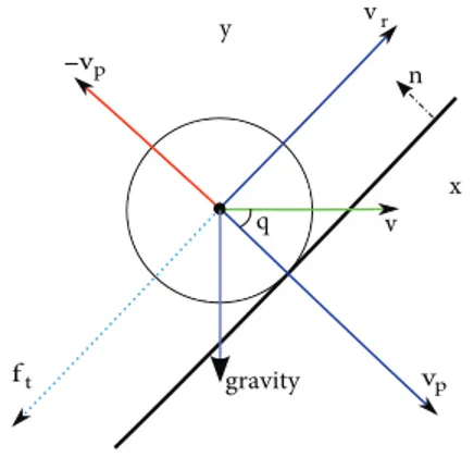
To resolve the collision in a realistic way, no penetration should be visible on the terrain. To ensure this, the velocity component of the particle, which is directly perpendicular to the collision plane, is diminished from the velocity vector. This is similar to the Neumann boundary condition [30], which enforces the following rule:

δv/δˆn = 0, (14)

where v is the velocity of the particle and ˆn is the normal vector of the collision plane. In addition to this, if

there is any penetration between the collision plane and particle, this is resolved by repositioning the particle by a vector in the direction of the plane normal according to the size of the penetration value. To better examine the situation, see Figure 2.

vp vp f_t y x n gravity v_r v q

Figure 2. Particle and collision plane.

The velocity component vp is negated and a lateral friction force ft is applied to the particle. The size

there is a bounce-back velocity added in the opposite direction of the plane normal. The reason for using the bounce-back velocity is to simulate an inelastic collision between the snow particles and terrain. Its actual value

is directly proportional to the size of vp.

The friction force is an adjustable variable to manipulate the way the particles interact with the terrain. Its length depends on the length of the velocity component that is parallel to the collision plane. For nonsmooth grained surfaces, this factor will have a velocity clamping effect against sliding. This can be used for various states of snow on the terrain, such as dry or slushy. The terrain also attracts the particles due to the fact that avalanches flow on layered snow, which may increase the viscosity of the flowing snow. This attraction force is

based on the following function, where ˆu is as in Eq. (13):

ˆ

v = ˆv + ˆu (15)

3.2. Rendering

There are many methods in the literature for rendering particle systems, such as Foster and Fedkiw’s level set method [31] and its derivatives by Enright [32] and Kim et al. [33], and Lorensen’s MCs algorithm [34] and its improvements [35–37], in addition to van derLaan et al.’s screen-space curvature flow method [38]. In order to render the scene, all meshes except for the particles are shaded using GLSL (OpenGL Shading Language) with vertex and fragment shader version 4.0 on the GPU [39]. The common algorithm used in the lightning of the meshes is the computing of the tangent space basis vectors in order to render shadowed objects more accurately [40,41]. Aside from the GLSL shaders and MCs, the Irrlicht 3D Rendering Engine version 1.7.1 is used as a baseline for all of the simulation rendering, including fast terrain rendering [42]. The following subsections describe the main rendering schemes used in the simulation in further detail.

3.2.1. Marching cubes

MCs have seen a lot of use for many particle systems that have obscure surfaces. In this paper, a parallel GPU implementation of MCs is used. The implementation is based on Nvidia’s MCs in software development kit examples [43]. The sampling is done depending on the amount and places of the particles in a voxel; the values for the edges of a voxel are increased according to the distance between the edge and the particle [see Figure 3

and Eq. (16)]. ∑ p=1...N    ∑ i=1...g m/gi    (16)

Here, gi is the distance between the center of the particle and the edges of the voxel, N is the total number

of particles in the neighboring cells, and m is the mass of the particle. This equation provides a value that is inversely proportional to the distance from the edges of the sampling cube. After the sampling process, the

MCs algorithm creates a surface geometry with the given sample data on a grid with a resolution of 128 × 128

× 128, with a voxel size of 1 unit.

The rendering of the resulting mesh is done via GLSL shaders with a lightning scheme similar to the terrain rendering described in [44]. In addition to this, there is a glittering postprocessing effect, which is based on the snow glittering effect for a gleaming look [45] (Figure 4).

g₁ g₂ g₅ g₆ g₇ g₈ g₃ cx,y,z g₄ Marching Cubes Voxel

Figure 3. Contribution of a particle to MCs’ sampling. Figure 4. Flowing snow with particle shading and MCs, at a render resolution of 128 × 128 × 128.

MCs have a dramatic impact on the performance of the simulation if the number of occupied voxels is high. This, of course, is related to the number of particles in the scene and adjoined in the flow, and the method used for sampling. Even though it slows down the simulation, it adds the volumetric appearance that a flowing avalanche requires. Further details about performance are given in Section 4.

3.2.2. Particle shaders

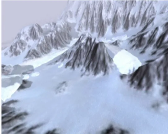
Particles are rendered as point sprites in the shape of small spheres and placed slightly on top of MCs’ mesh, which gives a granular look to a volume of flowing snow. The size of the particles adjusts linearly according to the distance between the viewpoint and particle position (Figure 5).

Figure 5. Particle rendering in the avalanche simulation.

3.2.3. Terrain and environment rendering

In the current simulation environment, the setting is on a snowy mountain, where layered snow has formed a thick layer below the avalanche zone. While the simulation takes place, the terrain does not deform or change shape, but rather provides a solid path and interacts with the particles by forming attraction bonds with them. For rendering the surface terrain and environment, light attenuation and ambient, diffuse, specular, and bump mappings are taken into account. Moreover, to give a realistic look, per-pixel fog is added as a postprocessing effect. The render pass of the terrain is handled by the Irrlicht rendering engine. The method used to render the terrain is based on level of detail rendering [46].

To add a bit of a realistic scenario, there is also a scenery effect, in which a set of ice slates/chunks fall off the cliff and the flowing snow is released afterwards. These ice chunks dislodge and fall to initiate the flowing

avalanche. They are predesigned as a whole mesh with links that are ready to be set broken. Currently, the particles do not interact with the ice slates, but it is possible to handle the interaction using methods such as triangle sampling or implicit sampling [47,48].

4. Results

In this paper, we present a method to simulate a flowing snow avalanche from over a mountain top to a recessive finish. To provide a faster performance, the underlying hardware’s capabilities are exploited. This includes using CUDA as a simulation environment and its tools for fast scanning of arrays and sorting. In addition to that, using OpenMP on the CPU side further establishes a faster rendering scheme as an optimization method. OpenMP is a multithreading application programming interface integrated into Visual Studio. The usage and applications are listed in [49].

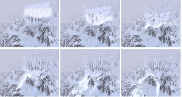
First, the simulation of a flowing avalanche without MCs and ice slates is presented (Figure 6). There

are 128 K (217) particles in the simulation and it runs at 40 fps on a Nvidia 8800GT graphics card with the

CUDA Toolkit 3.0 (March 2010) installed.

Figure 6. Flowing avalanche set loose on a mountainous terrain.

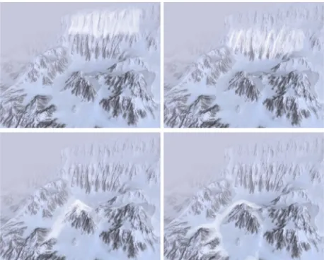
Another scheme (Figure 7) of a flowing avalanche is presented below. In this case, in addition to particles, MCs are utilized to obtain a volumetric view. Particles interact the way they do in the previous scheme, only

the MCs’ rendering is placed on top. There are 128 K (217_{) particles and it runs at 17 fps on a Nvidia 8800GT}

graphics card with the CUDA Toolkit 3.0 installed.

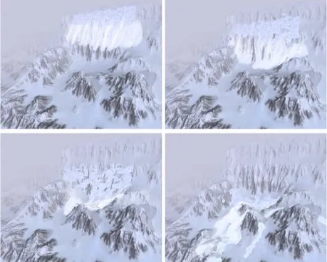
The last scheme (Figure 8) has a set of ice slates/chunks falling before the avalanche takes place. The chunks only interact with the terrain, independent from the particle system. The collision handling is done with a physics solver that works on the CPU. There are 128 K (217) particles and 232 individual ice slates that disentangle and slide on the terrain. It runs at 15 fps with the same system setup (Figures 9 and 10).

Figure 7. Flowing avalanche set loose on a mountainous terrain. Rendering includes MCs.

Figure 8. Flowing avalanche set loose on a mountainous terrain. Rendering includes MCs and ice chunks.

This implementation of a flowing avalanche simulation can provide interactive frame rates for 512 K

(219_{) particles. This is mainly thanks to the parallel architecture of a GPU and avoidance of serialization of}

0 5 10 15 20 25 30 35 40 45 128K 256K 512K 1024K

Frames per second

Number of particles

Particle only Particle & marching cubes

Particle, marching cubes, & ice chunks

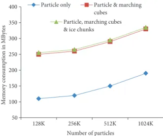
50 100 150 200 250 300 350 400 128K 256K 512K 1024K Me mory consumpt ion in MByt es Number of particles Particle, marching cubes & ice chunks

Particle only Particle & marching cubes

Figure 9. Simulation performance in frames per second with different sizes of particle sets and types of renderings.

Figure 10. Exact values of the simulation performance in frames per second with different sizes of particle sets and types of renderings with memory consumption.

5. Conclusion and improvements

This paper proposes a method for simulating one of the natural phenomena, a flowing avalanche, utilizing a MD-based DEM. By choosing a discrete simulation method, which can simulate granular material, rather than a holistic method such as SPH, we aim to add granular detail to a flowing avalanche. The color and rendering method of the particles, usage of MCs, and environment rendering are aimed to create a realistic simulation of an avalanche.

In order to exploit the parallelizability of the particle system, Nvidia’s CUDA architecture and Open MP are utilized. This is partially established using aligned texture memory in the graphics card for the CUDA computations and parallelizing the correct section of the code, while leaving the nonparallelizable code serial.

We choose rendering methods that are easy to implement and visually good-looking when used with at least 128 K particles, due to the fact that interactive rates can be achieved even when 512 K particles are in the system. The system we use has the following specifications: CPU, Intel Q6600 @ 3.0 GHz; memory, 3 GB DDR2 RAM; GPU, Nvidia 8800GT G92 512 MB; and CUDA Capable Cores, 112.

Possible improvements for the simulation include using a greater terrain size or multiple terrains that can be dynamically loaded from the CPU to the GPU in order to create a vast and even seamless terrain space without wasting GPU memory. Another improvement would be introducing real freeze bonds according to the snow bonds that are tracked in the GPU at each simulation step. By doing so, we may be able to simulate the dry and icy granular snow more realistically. Moreover, fracturing of a stiff snow pack would be possible to simulate with that method. Finally, the addition of obstacles such as trees or rocks on the path of the avalanche via adding a robust coupling method of the particle system with rigid bodies can be beneficial.

Many improvements for rendering methods are possible. For instance, by utilizing GPU-based

ray-casting algorithms and screen-space curvature flow [38] on particles, one can achieve a smooth and adjustable level of detail in particle rendering for slushy or dry avalanches. The addition of snow powder smoke to the simulation might improve realism even though this is not a mixed motion avalanche, which possesses airborne snow particles. Additionally, more optimized sampling methods can be introduced for calculating the dataset of the MCs.

References

[1] E.J. Hastings, R.K. Guha, K.O. Stanley, “Interactive evolution of particle systems for computer graphics and animation”, IEEE Transactions on Evolutionary Computation, Vol. 13, pp. 418–432, 2009.

[2] S. Bayraktar, U. Gudukbay, B. Ozguc, “Particle-based simulation and visualization of fluid flows through porous media”, Journal of Visualization, Vol. 13, pp. 327–336, 2010.

[3] T. Poschel, V. Buchholtz, “Molecular dynamics of arbitrarily shaped granular particles”, Journal de Physique I, Vol. 5, pp. 1431–1455, 1995.

[4] J. Monaghan, “Smoothed particle hydrodynamics”, Annual Review of Astronomy and Astrophysics, Vol. 30, pp. 543–574, 1992.

[5] N.J. Balmforth, A. Provenzale, Geomorphological Fluid Mechanics, Lecture Notes in Physics Vol. 582, New York, Springer, 2001.

[6] Z.H. Wan, Z. Wang, Hyperconcentrated Flow, London, Taylor & Francis, 1994.

[7] A.K. Patra, A.C. Bauer, C.C. Nichita, E.B. Pitman, M.F. Sheridan, M. Bursik, B. Rupp, A. Webber, A.J. Stinton, L.M. Namikawa, C.S. Renschler, “Parallel adaptive numerical simulation of dry avalanches over natural terrain”, Journal of Volcanology and Geothermal Research, Vol. 139, pp. 1–21, 2003.

[8] P. Gauer, D. Issler, K. Lied, K. Kristensen, F. Sandersen, “On snow avalanche flow regimes: Inferences from observations and measurements”, Proceedings of the International Snow Science Workshop, Vol. 1, pp. 717–723, 2008.

[9] T. Zwinger, “A simulation model for dry snow avalanches”, Proceedings of 28th IAHR Congress, pp. 22–27, 1999. [10] D. Issler, Flow Regimes in Snow Avalanches: New Insights and Their Possible Consequences, Vol. 1, Turin,

Associazione Georisorse e Ambiente Torino, 2006.

[11] C. Acary-Robert, D. Dutykh, D. Bresch, Numerical Simulation of Powder-Snow Avalanche Interaction with an Obstacle, Vienna, WPI, 2009.

[12] A. Kapler, “Avalanche! Snowy fx for xxx”, ACM SIGGRAPH’03 Sketches and Applications, Vol. 1, p. 1, 2002. [13] T.Y. Kim, L. Flores, “Snow avalanche effects for Mummy 3”, ACM SIGGRAPH 2008 Talks, Article No. 7, 2008. [14] Y. Tsuda, Y. Yue, Y. Dobashi, T. Nishita, “Visual simulation of mixed-motion avalanches with interactions between

snow layers”, The Visual Computer, Vol. 26, pp. 883–891, 2010.

[15] R. Gingold, J. Monaghan, “Smoothed particle hydrodynamics - theory and application to non- spherical stars”, Royal Astronomical Society Monthly Notices, Vol. 181, pp. 375–389, 1977.

[16] M. Muller, D. Charypar, M. Gross, “Particle-based fluid simulation for interactive applications”, Eurograph-ics/SIGGRAPH Symposium on Computer Animation, pp. 154–159, 2003.

[17] J. Stam, “Real-time fluid dynamics for games”, Proceedings of the Game Developer Conference, 2003.

[18] N. Bell, Y. Yu, P.J. Mucha, “Particle-based simulation of granular materials”, Proceedings of the ACM SIG-GRAPH/Eurographics Symposium on Computer Animation, pp. 77–86, 2005.

[19] B. Adams, M. Pauly, R. Keiser, L.J. Guibas, “Adaptively sampled particle fluids”, Proceedings of the ACM, Vol. 26, pp. 1–7, 2007.

[20] Y. Mike, Q. Froemke, “Ticker tape: a scalable 3d particle system with wind and air resistance”, available at http://software.intel.com/en-us/articles/ticker-tape-a-scalable-3d-particle- system-with-wind-and- air-resistance/, INTEL, 2010.

[21] J. Kruger, P. Kipfer, P. Konclratieva, R. Westermann, “A particle system for interactive visualization of 3d flows”, IEEE Transactions on Visualisation and Computer Graphics, Vol. 11, pp. 744–756, 2005.

[22] K. Hegeman, N.A. Carr, G.S.P. Miller, “Particle-based fluid simulation on the GPU”, Lecture Notes in Computer Science, Vol. 3994, pp. 228–235, 2006.

[23] T. Harada, S. Koshizuka, Y. Kawaguchi, “Smoothed particle hydrodynamics on GPUs”, Proceedings of the 25th Computer Graphics International Conference, pp. 63–70, 2007.

[24] S. Green, “Cuda particles”, available at http://developer.download.nvidia.com/compute/cuda/sdk/website/C/src/ particles/doc/p articles.pdf, Nvidia, 2007.

[25] M. Teschner, B. Heidelberger, M. Muller, D. Pomeranets, M. Gross, “Optimized spatial hashing for collision detection of deformable objects”, Proceedings of Vision, Modeling and Visualization, pp. 47–54, 2003.

[26] S. Melax, “Dynamic plane shifting BSP traversal”, Canadian Human-Computer Communications Society, pp. 213– 220, 2000.

[27] M. Teschner, S. Kimmerle, B. Heidelberger, G. Zachmann, L. Raghupathi, A. Fuhrmann, M.P. Cani, F. Faure, N. Manenat-Thalmann, W. Strasser, P. Volino, “Collision detection for deformable objects”, Computer Graphics Forum, Vol. 24, pp. 61–81, 2005.

[28] N. Satish, M. Harris, M. Garland, “Designing efficient sorting algorithms for many-core GPUs”, Proceedings of the IEEE International Symposium on Parallel & Distributed Processing, pp. 1–10, 2009.

[29] E.W. Weisstein, “Point-plane distance from MathWorld–a Wolfram web resource”, available at http://mathworld.wolfram.com/Point-PlaneDistance.html, MathWorld, 2010.

[30] A.H.D. Cheng, D.T. Cheng, “Heritage and early history of the boundary element method”, Engineering Analysis with Boundary Elements, Vol. 29, pp. 268–302, 2005.

[31] N. Foster, R. Fedkiw, “Practical animation of liquids”, Proceedings of the 28th Annual Conference on Computer Graphics and Interactive Techniques, Vol. 20, pp. 23–30, 2001.

[32] D. Enright, S. Marschner, R. Fedkiw, “Animation and rendering of complex water surfaces”, ACM Transactions on Graphics, Vol. 21, pp. 736–744, 2002.

[33] J. Kim, D. Cha, B. Chang, B. Koo, I. Ihm, “Practical animation of turbulent splashing water”, Eurographics/ACM SIGGRAPH Symposium on Computer Animation, pp. 335–344, 2006.

[34] W.E. Lorensen, H.E. Cline, “Marching cubes: a high resolution 3d surface construction algorithm”, Proceedings of the 14th Annual Conference on Computer Graphics and Interactive Techniques, Vol. 16, pp. 163–169, 1987. [35] E.V. Chernyaev, “Marching cubes 33: construction of topologically correct isosurfaces”, Technical Report CERN

CN 95-17, Geneva, CERN, 1995.

[36] G.M. Nielson, B. Hamann, “The asymptotic decider: resolving the ambiguity in marching cubes”, Proceedings of the IEEE Conference on Visualization, pp. 83–93, 1991.

[37] A. Lopes, K. Brodlie, “Improving the robustness and accuracy of the marching cubes algorithm for isosurfacing”, IEEE Transactions on Visualization and Computer Graphics, Vol. 9, pp. 16–29, 2003.

[38] W.J. Van der Laan, S. Green, M. Sainz, “Screen space fluid rendering with curvature flow”, Proceedings of the Symposium on Interactive 3D Graphics and Games, pp. 91–98, 2009.

[39] R.J. Rost, B.M. Licea-Kane, D. Ginsburg, J. Kessenich, B. Lichtenbelt, H. Malan, M. Weiblen, OpenGL Shading Language, New York, Addison-Wesley Professional, 2009.

[40] L. Eric, “Computing tangent space basis vectors for an arbitrary mesh”, available at http://www.terathon.com/code/tangent.html, Terathon Software 3D Graphics Library, 2001.

[41] D.G. Luenburger, Optimization by Vector Space Methods, New York, Wiley, 1997.

[42] Irrlicht, “Irrlicht rendering engine”, available at http://sourceforge.net/projects/irrlicht, 2010.

[43] Nvidia, “Marching cubes isosurfaces”, available at http://www.nvidia.com/content/cudazone/cuda sdk/Physically-Based Simulation.htm, Nvidia, 2010.

[44] J. Guinot, “Bump mapping using GLSL”, available at http://www.ozone3d.net/tutorials/bump mapping p3.php, OZONE3D, 2010.

[45] AMD, “AMD rendermonkey toolkit tutorials”, available at http://developer.amd.com/archive/gpu/rendermonkey/ pages/default.asp, 2010.

[46] P. Lindstrom, D. Koller, W. Ribarsky, L.F. Hodges, N. Faust, G.A. Turner, “Real-time, continuous level of detail rendering of height fields”, Proceedings of the 24th Annual Conference on Computer Graphics and Interactive Techniques, Vol. 15, pp. 109–118, 1996.

[47] A. Witkin, P.S. Heckbert, “Using particles to sample and control implicit surfaces”, Proceedings of the 21st Annual Conference on Computer Graphics and Interactive Techniques, Vol. 24, pp. 269–277, 2005.

[48] G. Turk, “Re-tiling polygonal surfaces”, Computer Graphics, Vol. 26, pp. 55–64, 1992.

[49] OpenMP Board, “The openmp api specification for parallel programming”, available at http://www.openmp.org, OpenMP, 2010.