A REGIONAL AND SECTORAL ANALYSIS ON PRODUCTION TECHNOLOGY DYNAMICS OF MANUFACTURING INDUSTRIES IN
TURKEY A Master’s Thesis by S ¨UMEYRA KORKMAZ Department of Economics
˙Ihsan Do˘gramacı Bilkent University Ankara
To my beloved husband Halil and my family
A REGIONAL AND SECTORAL ANALYSIS ON PRODUCTION TECHNOLOGY DYNAMICS OF MANUFACTURING INDUSTRIES IN
TURKEY
Graduate School of Economics and Social Sciences of
˙Ihsan Do˘gramacı Bilkent University
by
S ¨UMEYRA KORKMAZ
In Partial Fulfillment of the Requirements For the Degree of MASTER of ARTS
in
THE DEPARTMENT OF ECONOMICS ˙IHSAN DO ˘GRAMACI B˙ILKENT UNIVERSITY
ANKARA September 2015
I certify that I have read this thesis and have found that it is fully adequate, in scope and in quality, as a thesis for the degree of Master of Arts in Economics.
Prof. Dr. Erin¸c Yeldan Supervisor
I certify that I have read this thesis and have found that it is fully adequate, in scope and in quality, as a thesis for the degree of Master of Arts in Economics.
Asst. Prof. F. Banu Demir Pakel Examining Committee Member
I certify that I have read this thesis and have found that it is fully adequate, in scope and in quality, as a thesis for the degree of Master of Arts in Economics.
Assoc. Prof. Hakan Ercan Examining Committee Member
Approval of the Graduate School of Economics and Social Sciences
Prof. Dr. Erdal Erel Director
ABSTRACT
A REGIONAL AND SECTORAL ANALYSIS ON PRODUCTION TECHNOLOGY DYNAMICS OF MANUFACTURING INDUSTRIES IN
TURKEY Korkmaz, S¨umeyra
M.A., Department of Economics Supervisor: Prof. Dr. A. Erin¸c Yeldan
September 2015
This thesis estimates regional and sectoral total factor productivity (TFP) using firm-level data on Turkish manufacturing industry over the 2003-2012 period to understand whether there is a parallelism between differences in TFP levels and differences in income per capita across regions. As propounded by Prescott (1998), TFP theory is utilized to explain international income differences in the existing literature. However, it still remains an interesting topic to study regional differences within countries and this thesis contributes to the literature with an empirical evidence from Turkey’s regions. Based on the results obtained from different estimation methods, there is a significant heterogeneity across sectors and firms in the same sector in the micro-level and this results in different average TFP levels for regions at macro-level. Our findings suggest that discrepancies in regional TFP levels are determined by technological dynamics of the industries that are dense in those regions. Thus, different sector abundance in different
regions may be one of the factors for different levels of income per capita among regions.
¨ OZET
T ¨URK˙IYE ˙IMALAT SANAY˙I ¨URET˙IM TEKNOLOJ˙IS˙I D˙INAM˙IKLER˙I ¨
UZER˙INE B ¨OLGESEL VE SEKT ¨OREL D ¨UZEYDE ANAL˙IZLER Korkmaz, S¨umeyra
˙Iktisat B¨ol¨um¨u, Y¨uksek Lisans Tez Danı¸smanı: Prof. Dr. Erin¸c Yeldan
Eyl¨ul 2015
Bu tez, 2003-2012 yılları i¸cin firma bazında T¨urkiye imalat sanayi verisi ile sekt¨orel ve b¨olgesel d¨uzeyde toplam fakt¨or verimlili˘gi tahminleyerek, b¨olgesel toplam fakt¨or verimlili˘gi farkları ile ki¸si ba¸sı gelir farkları arasında ba˘gıntı olup olmadı˘gına bir cevap aramaktadır. Prescott (1998) tarafından ¨one s¨ur¨ulen toplam fakt¨or verimlili˘gi teorisi, ¸simdiye kadar yapılan ¸calı¸smalarda uluslararası gelir fark-larını a¸cıklamak i¸cin kullanıldı. Fakat, b¨olgesel d¨uzeyde farklılıklar alanında daha fazla ¸calı¸sma yapılması gerekmektedir. Bu tez, varolan literat¨ure T¨urkiye’nin b¨olgesel analizi ile ampirik bir katkıda bulunmaktadır. Firma bazında tahminleme yapılırken kullanılan farklı y¨ontemlerle elde edilen sonu¸clara g¨ore, mikro d¨uzeyde firma farklılıkları, ortalama toplam fakt¨or verimlili˘ginde makro d¨uzeyde b¨olgesel farklara sebep olmaktadır. Elde edilen bulgular b¨olgeler arası g¨or¨ulen toplam fakt¨or verimlili˘gi farklılıklarınn sebebi olarak b¨olgelerde yo˘gun olarak faaliyet g¨osteren sekt¨orlerin farklı teknolojik dinamiklere sahip olmasını ortaya koymak-tadır. Sonu¸c olarak, farklı b¨olgelerde farklı sekt¨orlerin yı˘gınla¸sması b¨olgesel ki¸si
ba¸sı gelir farklarını a¸cıklayıcı bir etken olabilir.
Anahtar kelimeler : firma seviyesinde veri, toplam fakt¨or verimlili˘gi, b¨olgesel kalkınma.
ACKNOWLEDGMENTS
I would like to thank my advisor Professor Erin¸c Yeldan for his great support and advice throughout this process and I want to thank Professor Hakan Ercan for his worthwhile comments as an examining committee member. Also, I am grateful to Professor Banu Demir Pakel for her sincerity, guidance in TUIK and useful feedbacks as examining committee member.
I want to express my appreciation to Professor Refet G¨urkaynak for his helpful comments and encouragement throughout my master study. I want to thank Dr. Seda K¨oymen ¨Ozer and Yasin Babahano˘glu for their useful comments and help in thesis writing process. I also want to thank TURKSTAT and its employees for providing the data and work environment.
Special thanks to all my family members, especially my sister for their moral and material support in my academic career.
Last but not the least; I would like to express the deepest appreciation to my beloved husband Halil for his effort during this academic process as my best friend and family. Experiencing the same process, he had a great empathy with me in this thesis writing process and he have made this period as easy and enjoyable as possible with all other friends in this graduate study.
TABLE OF CONTENTS
ABSTRACT . . . iii
¨ OZET . . . v
ACKNOWLEDGMENTS . . . vii
TABLE OF CONTENTS . . . viii
LIST OF FIGURES . . . x
LIST OF TABLES . . . xi
CHAPTER 1: INTRODUCTION . . . 1
CHAPTER 2: LITERATURE REVIEW . . . 4
2.1 Literature Review on Turkey TFP Estimation . . . 5
2.2 Literature Review on Misallocation . . . 6
2.3 Literature Review on TFP Estimation Techniques . . . 8
CHAPTER 3: DATA AND METHODOLOGY . . . 11
3.1 Description of Data . . . 12
3.1.1 Dependent Variables . . . 12
3.1.2 Independent Variables . . . 12
3.1.3 Proxy Variables . . . 14
3.2 Methodology . . . 15
3.2.2 Methodology for Levinsohn-Petrin Approach . . . 17
CHAPTER 4: EMPIRICAL RESULTS . . . 20
4.1 Comparison of Different Estimation Coefficients . . . 20
4.2 Regional TFP Levels . . . 21
4.3 Robustness Check for Capital . . . 23
CHAPTER 5: CONCLUSION . . . 25
BIBLIOGRAPHY . . . 27
APPENDIX . . . 30
LIST OF FIGURES
1 Per Capita Gross Value Added of Regions to Turkish Economy . . 44
2 Distribution of Employed People by Economic Activity . . . 44
3 Distribution of Income by Deciles . . . 45
4 TR41-Manufacture of Transportation Equipment . . . 45
5 TR32- Textile Products . . . 46
6 TR32- Manufacture of Wearing Products . . . 46
7 TR63- Textile Products . . . 47
8 TR63- Basic Metal Industry . . . 47
9 TR72- Manufacture of Furniture, Building and Repairing . . . 48
10 TRA1- Manufacture of non-metallic Minerals . . . 48
11 TR42- Manufacture of Rubber and Plastics . . . 49
12 TR42- Basic Metal Industry . . . 49
13 TR42- Manufacture of Fabricated Metals (except machinery) . . . 50
14 TR42- Manufacture of Chemicals and Chemical Products . . . 50
LIST OF TABLES
1 Sectors value added for Turkey (Percentage to GDP) . . . 30 2 Manufacturing Industry List . . . 30 3 Region Classifications at NUTS2 Level . . . 31 4 Domestic Producer Price Index, Main Industrial Groupings . . . . 32 5 Domestic Producer Price Index- Sections, Divisions . . . 32 6 Summary Statistics by Year . . . 33 7 Summary Statistics by Sectors . . . 33 8 Number of Enterprises in Each Region and Average TFP levels . 34 9 Number of Enterprises in Each Region and Average TFP levels . 35 10 OLS Estimates of Production Function for Each Regions,
Depen-dent Variable: Value Added . . . 36 11 FE Estimates of Production Function for Each Regions, Dependent
Variable: Value Added . . . 37 12 OP Estimates of Production Function for Each Regions, Dependent
Variable: Value Added . . . 38 13 LP Estimates of Production Function for Each Regions, Dependent
Variable: Value Added . . . 39 14 Classification of Manufacturing Industries According to Technology
Intensity . . . 40 15 Robustness Check for Capital . . . 41 16 T-test for CRTS . . . 42 17 Regional Household Average and Median Disposable Income (Yearly) 43
CHAPTER I
INTRODUCTION
A popular question in macroeconomics is, “why are some countries richer than others?”. Not surprisingly, there is a rich literature providing a variety of answers. It still remains an interesting topic to study regional differences within countries rather than aggregated national data, since within country income distribution gives a clear idea about the country’s level of development.
Many theorists try to model long run growth path of economies. Since the sem-inal work of Barro et al. (1991), convergence of income levels between countries or between regions of the same country draws the attention of many researchers (Blanchard and Katz, 1992; Sala-i-Martin, 1996). However, most of the time, het-erogeneity across sectors and regions of the country remains in the background. The presence of such heterogeneity across sectors or regions could result in sev-eral outcomes, one of which is total factor productivity (TFP) differences among these sectors/regions and the other is misallocation of resources. These outcomes have been put forward as reasons for within-country income per capita differences (Restuccia and Rogerson, 2008; 716-720). In this thesis, I will analyze dynamics of regional and sectoral production technology in the manufacturing industries
in Turkey using a panel data approach in order to examine whether TFP levels provide insight about different degrees of development within Turkey.
Understanding the characteristics of Turkey’s regions is crucial, since it gives the motivation for this thesis. Figures 1,2 and 3 present an overview of Turkish re-gions based on data provided by Turkish Statistical Institute (TURKSTAT). For simplicity, I have aggregated data into three subgroups as high-income, middle-income and low-middle-income regions according to their per capita gross domestic prod-uct levels of provinces in 2011. In Figure-I, apparently there is a huge difference between regions’ participation to gross value added. The comparison between years 2004 and 2011 shows that there is an improvement in all regions over time.
To see the reason behind this variation between regions, Figure-2 could provide a clarification, in which economic activity of employment in percentage is shown. As seen in Figure-2, low income regions give more weight to agriculture than high-income regions, which has a lower value added compared to industry or service sectors. On the contrary, high income regions concentrate on services more than other regions. While considering the value added of these sectors as reported in Table-1, it is expected to see less value added in regions where agriculture plays a significant role.
Also in Figure-3, we observe that there is a large difference between disposable incomes of last deciles in three sub-regions. According to the per capita gross domestic products (GDP) of provinces, there is a sharp economic divide between northeast and the rest of the country. Thus, I divided the country into three sub-regions.
All the reasons I have mentioned above stimulate the assertions about misal-location, geography and “agglomeration effect” that Krugman (1990) and others
(Acemoglu et al. 2001, Restuccia et al. 2013) have put forward. As in Prescott (1998) and Hall and Jones (1999), I will mainly focus on estimation of regional and sectoral TFP using data on Turkish manufacturing firms to observe whether the dominant source of differences in output per worker is caused by differences in TFP levels.
The rest of the thesis is organized as follows. In the next chapter 2, summary of some key contributions from existing literature including estimation techniques is provided. Data and methodology are described in the third chapter. Chap-ter 4 discusses the estimation results and chapChap-ter 5 concludes with some policy recommendations.
CHAPTER II
LITERATURE REVIEW
In the first place, we can start with the origins of TFP traced back to Solow (1957). In his seminal paper, he defines change in the technology as “any kind of shift” in the production function, but he focuses on different saving rates to give an explanation for international income differences. As a follow-up, Lucas (1988) introduces the concept of human capital as schooling, experience or specializing to elucidate income differences between countries and he takes the neoclassical growth model a step further. However, Prescott (1997) finds earlier works un-satisfying since he shows evidence that the same level of human capital cannot explain international income differences. That’s why, he uses total factor produc-tivity theory to clarify international and within country income differences.
After the seminal work of Prescott, the idea of productivity is used to explain developed and developing countries’ income levels or TFP approach is utilized to compare per capita income differences among countries after-trade income lev-els. Grossman and Helpman (1991), is one of the examples that model a close economy in which productivity increases after trade liberalization since the in-teraction between trading countries trigger knowledge and innovation spillovers.
Caselli (2005), endeavors to clarify cross-country income differences not only with factors of production but also with differences in efficiency levels using survey data from both OECD and non-OECD countries. He claims that differences in human capital or physical capital are not enough to explain income inequality, but efficiency would be the biggest part of the answer to the question. In addi-tion, Sivadasan (2006) uses plant-level data on Indian manufacturing sectors to analyze increase in productivity following foreign direct investment (FDI) liber-alization and tariff liberliber-alization. His results reveal that productivity increases by more than 25 percent after both liberalization periods. Therefore, the results are consistent with the Grossmann et al. (1991) assertion about the knowledge spillovers. Having a far-reaching data set, Gennaioli et al. (2014) analyze 83 countries regional growth and convergence rates, including Turkey, over the pe-riod 1975-2001. They conclude that regional growth is shaped by national growth and countries with better regulation exhibit faster convergence. They study the slow convergence issue of subnational regions; however they could not understand the reasons behind it and advice to focus on technological dynamics of the regions.
2.1 Literature Review on Turkey TFP Estimation
To continue with the existing literature on Turkish TFP estimation, Atiyas and Bakıs (2013) provide us with an aggregate and sectoral TFP growth analysis in their recent work. Their findings show that TFP growth in Turkey after 2000s is more than 3 percent, and agriculture sector exhibits strikingly higher TFP growth than industry sector . They also compare the TFP levels in Turkey with some other 98 countries. However, the results could be biased since they use aggregated data and estimate TFP by Ordinary Least Squares Method only for three main sectors. Again, in his empirical work Filiztekin (2000) analyzes the productivity
growth in Turkish manufacturing sectors after trade liberalization. In opposition to neoclassical growth theories, he finds a significant effect of openness to trade on productivity and growth. Yet, he uses the data up until year 2000 and his methodology is problematic while estimating TFP levels due to some endogeneity problems.
Aggregated data and endogeneity problems are also encountered in Saygılı et al. (2005) and Taymaz et al. (2008) where they use Ordinary Least Squares (OLS) estimation, fixed-effect method or GMM estimation of Cobb-Douglas pro-duction function with aggregated data. Focusing on the capital accumulation to explain sources of economic growth, Saygılı et al. ascertain that there is a pos-itive correlation between economic growth and capital accumulation. Also, they claim that productivity indicators are weak for agriculture and services sectors, whereas it is high for industry sector. Both papers, draw attention to the increase in productivity with structural transformation after 2000s. While, all the papers I have reviewed above give a general idea about TFP levels, they do not provide a detailed analysis and they do not properly estimate TFP with an aim to explain regional income differences. Time interval, usage of aggregated data and method-ological problems show that there is a need to estimate regional TFP using more recent and detailed data, a gap that this thesis aims to fill.
2.2 Literature Review on Misallocation
Apart from total factor productivity approach to explain differences in income per capita for countries or regions in a country, there is also an extensive literature on misallocation that investigates the regional differences within national bound-aries. After the seminal work of Krugman (1990), in which distinct regions within a country are analogous to core and periphery dichotomy, many researchers have
concentrated on the misallocation subject. In their paper “Agglomeration in the Global Economy” , Ottaviano and Puga (1997) analyze the share of sectors in each region and their input levels. What they conclude is that even if the regions are homogeneous ex-ante, more productive labors migrate from less productive regions, where agriculture is the main source of living, to more productive regions where industry or the services sectors are the main source of living. This creates a discrepancy in productivity levels of inputs across regions ex-post. After a while, some part of the world will function as a core whereas the other parts will be poor periphery. Also Acemoglu et al. (2001) highlight the impact of geography and institutions on the world income distribution and conclude that the region that institutionalized earlier has an advantage over the other regions that results in geographical per capita income differences.
Additionally, Jones (2011) explores the effect of misallocation of resources on different TFP levels and income differences. His paper not only provides empirical evidence from OECD countries, but also constructs a simple two-good economy model where inputs are allocated differently. He claims that the misallocation of resources at the micro-level results in different TFP levels at macro-level. Finally, Restuccia and Rogerson (2013) use the misallocation argument to explain the total factor productivity differences as a reason for the income differences. Get-ting to the main reason for income differences, they conclude that misallocation of resources driven by heterogeneity of firms/regions or distortions/externalities creates differentiation in efficiency across regions, thereby creating differences in income per capita across regions.
As mentioned in the first chapter, misallocation and TFP levels are argued to be the main reasons for income distribution. Recently availability of firm-level data and new estimation techniques stimulate the interest for TFP calculations
and using region and sector specific data, it is possible to differentiate dynamics of the regional and national economies. In what follows, this thesis contributes to Turkish TFP estimation literature by utilizing firm-level data provided by TURKSTAT at regional (NUTS-2) and industry (NACE-2) levels, and using new estimation techniques.
2.3 Literature Review on TFP Estimation Techniques
Estimating TFP as residual from OLS estimation can create simultaneity since choices of inputs, such as labor, can be correlated with the unobserved productiv-ity shock to the firm. Also in the balanced panel data, we only observe surviving firms over time, which may cause a selection bias. Therefore, estimating TFP with OLS method can cause endogeneity or selection bias problems (Van Bev-eren, 2012). There are some methods to get rid of simultaneity problem like instrumental variable (IV) estimation, fixed-effect (FE) (Mundlak, 1961; Hoch, 1962) or random-effect panel estimation. However, they all have some drawbacks in estimation process. For example, in fixed-effect estimation error term is divided into two parts, one of which is a time-invariant and firm specific ωi, to solve the
simultaneity problem with the following form.
yit= β0+ βkkit+ βllit+ βmmit+ ωi+ ηit
However, it needs the assumption of strict exogeneity,
E(yit|lit, kit, mit, ωi) = β0 + βllit+ βkkit+ βmmit+ ωi
unless it causes inconsistency and bias towards to zero in the estimation and this assumption does not hold in practice (Van Beveren, 2012). Whereas, IV method
does not need strict exogeneity assumption for consistent estimation. In this method a variable correlated with inputs and uncorrelated with the shock such as input prices is essential, but most of the time input prices are not observed or even if it is observed, firms with market power set their input prices according to their productivity and sales, so input prices become endogenous. Lagged levels of inputs can also be used as instruments. But this approach introduces a downward bias in the estimates of the coefficient of the capital input (Van Beveren, 2012). Therefore, Blundell and Bond (2000) introduce generalized method of moments (GMM) for more accurate estimates defining AR(1) process for a part in error term. Although GMM is a proper solution for endogeneity problem, it is not sufficient to deal with selection bias issue since it does not take survival probability of firms into account.
To correct the endogeneity and selection problems and to obtain more ac-curate estimates, there are some dynamic models used for firm-level data such as Olley and Pakes (1996) and Levinsohn and Petrin (2003). Working with the telecommunications equipment industry data, Olley and Pakes (OP) suggest that reallocation of capital towards more productive plants after regulation in the in-dustry causes an increase in the productivity. They propose a model in which investment is chosen as proxy variable in order to get rid of endogeneity problem. They also suggest a solution to selection bias problem. While other balanced panel data methods require the existence of all firms in all years, Olley and Pakes argue that exit or entry decisions of firms depend on their future productivity. Therefore, they develop an algorithm in which at every period each firm decides whether to exit or continue according to their expected productivity level and if it exits it never re-enters. However the assumptions needed for Olley and Pakes method are too restrictive that only firms with non-zero investment levels can be included in the sample. Since in most of the developing countries data, including
Turkey, firms report zero investment, it is not a suitable method to use for Turkish TFP estimation.
In addition, Levinsohn and Petrin (LP) propose a technique in which they use intermediate materials as proxy in order to prevent endogeneity using Chilean manufacturing data (2003). While in most countries firms report zero investment, they report their use of material or energy, such as electricity and fuel. There are also other extensions to these models and there is no surely correct method since the data and assumptions should match in order to favor a method over others. Due to the structure of Turkey manufacturing data; I will be utilizing LP method to estimate TFP levels and the details about this method will be given in the next chapter.
CHAPTER III
DATA AND METHODOLOGY
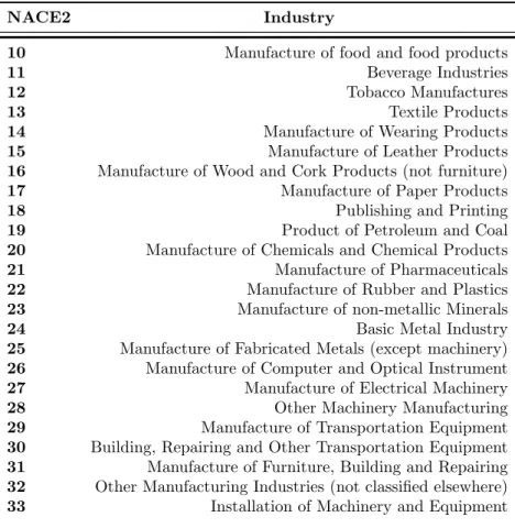
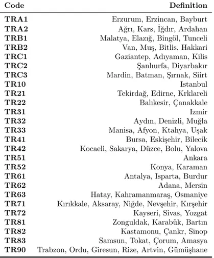
The data set used in this thesis is provided by TURKSTAT and available only in the data research center of the institute. Data is collected from enterprises which have 20 or more employees at the end of every year. The survey covers between the years 2003 and 2012. The institute also has data for years between 1980 and 2001, but the structure of the surveys and data collection methods are completely different so that I could not use data before 2003. Also main activity codes of the firms at NACE2 level are available and the description of each sectoral activity is given in Table-2. Since manufacturing industry data does not include the regions of the firms, I used local unit micro data to obtain the location of the firms at NUTS2 level by matching identity numbers of enterprises and Table-3 specifies the provinces included in each region. Table-6 gives the summary statistics of the available data by years including number of enterprises, number of employed persons and production values.
3.1 Data
3.1.1 Dependent Variables
Production value of the firms included in the data set is measured as the sum of annual sales and changes in the stock value of final products for that year. According to their sectoral inflation rates reported in Table-5 at 2-digit level, production value is deflated at base year 2003. Deflating the production value with own sector prices is a substantial factor since in some sectors there is 500% inflation over a period of 10 years such as petroleum and coal, whereas in some sectors price level decreases each year like pharmaceuticals.
Other dependent variable used in the estimations is value added with factor prices provided by TURKSTAT and it is also deflated by corresponding sector prices.
3.1.2 Independent Variables
Labor as an indispensable factor of production is given for firms in every year as total number of hours worked. The number of workers are also included in the data set, but there are different types of employees as full-time and part-time and the hours they work is not the same, so that I used number of hours worked for the sake of unity in all firms. Unfortunately, after 2001 there is no information about the skills, education levels or service area of the employees as white collar or blue collar. Therefore, there is only one type of labor in the estimation.
Another main factor for production, capital, is not reported in the survey data. Hence, it is estimated using investment data of firms which is reported
separately as investments on machinery/equipment, patents/computer program-ming and building/structure. After deflating the investment series with relevant price deflators, capital stocks for each item is constructed with perpetual inven-tory method. Before applying the method, an assumption is needed for the initial capital stock estimation, that is firms’ being at their balanced growth path.
Considering Ki0 as initial capital stock of firm i and δ as depreciation rate, we
can write
Ki1 = (1 − δ)Ki0+ Ii0 (1)
Dividing both sides of equation 1 with Ki0, we get
Ki1/Ki0 = (1 − δ) + Ii0/Ki0 (2)
Since we have assumed that firms are at their balanced growth path
Ki1/Ki0= Yi1/Yi0 = 1 + gi (3)
where g is the growth rate of the firm and calculated as growth of deflated production value, we get
K0 = I0/(gi+ δ) (4)
Since I have different depreciation rates for different investment types, I con-structed capital for building using δ=5%, for machinery δ=10% and for patent δ=30% (Yılmaz and ¨Ozler, 2005).
In the data set, not all firms report positive investment for first year they appeared in the data set, for this reason I have taken the first year reported with
positive investment to calculate initial capital stock and iterated back for former years with 1/(1-δ) for each type of capital stock.
Calculating the initial capital, perpetual inventory method is used for following years where,
Kt+1 = (1 − δ)Kt+ It (5)
Finally, aggregating the different capital stock of each firm, total capital for each year is constructed.
Another independent variable included in the estimates is material input calcu-lated as value of purchases on intermediate inputs plus the change in the material input stock for that year and deflated by corresponding inflation rates in Table-4.
3.1.3 Proxy Variables
Starting with Olley-Pakes (OP) methodology, it is needed to use investment as a proxy to elucidate endogeneity problem mentioned earlier. Aggregated in-vestment of the firm is used for this estimation. On the contrary, Levinsohn-Petrin (LP) mention zero investment reported in firm-level data to demonstrate the problem in OP method, especially for developing countries. Since the obser-vation number is decreasing with investment as proxy, they suggest energy to be used as a proxy in the estimation which is a variable reported non-zero by most of the firms.
In my data set 1/4 of the observations are excluded when OP approach is applied to production function due to zero investment entries. Therefore, LP approach is more proper to apply with available data set of Turkey. I will use
both techniques to give empirical evidence to Levinsohn and Petrin’s objective to Olley and Pakes where estimate results are biased.
In addition, we need exit variable for OP estimation which equals 1 if the firm exited at the beginning of that period and 0 otherwise.
Another proxy variable used in LP estimation is energy and calculated as the purchases on electricity and fuel minus the revenues from energy. It is also deflated with energy prices reported in Table-4.
3.2 Methodology
Assuming that the production function of the firms take Cobb-Douglas pro-duction function form,
Yit = AitKitβkL βl
itM βm
it (6)
where Yit stands for output of firm i at time t as dependent variable and Kit,
Lit and Mit are capital, labor and material inputs of firm i at time t, respectively.
Aitstands for the productivity level which is unobserved to the researcher whereas
other independent variables are observable.
Taking the natural logarithm of production function in equation 6,
yit= β0+ βkkit+ βllit+ βmmit+ εit (7)
we get logarithmic form of production function where lower case letters correspond to natural logarithms of each variables.
β0 and time and firm specific measurement error of TFP, εit.
3.2.1 Methodology for Olley-Pakes Approach
As mentioned earlier, estimating those coefficients with OLS can cause endo-geneity since the time and firm specific shock to productivity is observed to the firm and can lead them to choose their inputs accordingly resulting in correlation between the coefficients and the shock. In addition to endogeneity, firms with lower productivity has higher probability to exit the market and average produc-tivity increases when they exit. As a result, entering to market afterwards become more difficult for new entrants (Melitz, 2003) and this situation causes selection bias in OLS estimation.
To overcome those problems, Olley and Pakes suggest a model where εit is
decomposed into an observable or forecastable component, ωit as a function of
productivity and capital and unobservable component ηit and production function
takes the form below.
yit = β0+ βkkit+ βllit+ βmmit+ ωit+ ηit (8)
Hence, β0 + ωit = ait. To solve for ait OP use exit variable, Xit following a
first-order Markov process mentioned in the description of data section to prevent selection bias problem in addition to a proxy variable as investment levels of firms. They claim that investment as a function of capital and productivity is strictly increasing in productivity so that its inverse exits. Taking the inverse of function iit = ht(kit, ait), productivity as an unobservable variable can be written as a
function of observables as ait = gt(kit, iit) where ht(.) = g−t 1(.).
using OLS method to consistently estimate βl and βm at first stage.
yit= βllit+ βmmit+ f (kit, iit) + ηit (9)
Using the estimated coefficients and taking survival probability into consider-ation, OP estimate βk in the second stage. Estimated productivity in OP method
can be constructed as residual from the following equation.
ˆ
ait= yit− ˆβkkit− ˆβllit− ˆβmmit (10)
After taking the exponential of ˆait, TFP is calculated at firm level for each
year. However, a severe truncation in the data is needed for OP method since 1/4 firms in my data set report zero investment and this fact could cause another type of selection bias. The estimation results for OP are reported in Table-12.
3.2.2 Methodology for Levinsohn-Petrin Approach
While Olley and Pakes suggest using investment as proxy variable so as to prevent endogeneity problem, Levinsohn and Petrin are aware of the fact that developing countries’ data contains lots of zero investment entries. Since firms report non-zero material input such as electricity and gas consumption, they sug-gest material input as a proxy in estimation (LP, 322). It is also possible to get healthier results than investment as a proxy since materials like electricity can respond better to productivity shock.
Again taking the same productivity function equation
and demand for material input positively depends on the firms state variable kt and at
mit = mt(kit, ait) (12)
Positive effect of aiton demand of mit allows the inversion of demand function
as
ait= nt(kit, mit) (13)
where mt(.) = n−t 1(.).
Therefore, unobserved productivity function becomes function of two observ-able inputs. LP also allow us to estimate TFP taking value added, vitas dependent
variable where
vit= β0+ βllit+ βkkit+ ωit+ ηit (14)
and TFP can be calculated as taking the exponential of following equality.
ˆ
ait = vit− ˆβkkit− ˆβllit (15)
The estimation process identified in the above includes two stages in which LP estimates first βl consistently and at the second stage βk is estimated and differs
from OP as taking material input as proxy.
Difference between taking two variables as independent arises when executing the regressions. In the case where production value is dependent variable, LP is unable to identify coefficients of variables due to lack of variation in the data (Arnold, 2005). Therefore, my estimation relies on value added approach of LP
estimation techniques tabulated in Table-13. I used value added in all estimation techniques to be able to compare results.
CHAPTER IV
EMPIRICAL RESULTS
In this section, the results of different estimation techniques and TFP estima-tion results are discussed using Tables 9-10-11 and 12.
4.1 Comparison of Different Estimation Coefficients
Arguing the possible problems of different estimation techniques in the above chapters, this section provides empirical evidence for those problems with Turkish manufacturing data. In Table-10, the coefficient estimates of production function with OLS are reported with significance levels for each region. Compared to other estimations’ coefficients, OLS gives higher values for labor which is expected. Since the positive correlation between productivity shock and labor choice, OLS results are biased upwards confirming the theoretical results. When capital co-efficients are examined, it is clear that OLS gives a downward bias that results underestimating the effect of capital in production.
The difference of fixed effect estimates with OLS and LP estimates can be explained by change in the magnitude of productivity shock of firms over time.
According to firm-level TFP estimation, what I observe is that firms’ productivity level changes over time but not with a constant rate. Therefore, our data does not properly fit to fixed-effect estimation model.
In Table-12 and Table-13, there is no apparent difference between the labor coefficients in some regions. On the other side, capital coefficients become distinct due to loss of information caused by zero investment reports of enterprises in OP estimation. In addition, there is a column named ”sum” corresponding to the sum of coefficients for each estimator and indicate almost constant returns to scale for OLS and decreasing returns to scale for FE.
As a superior estimation technique, LP results give more clear idea about the economies of scale for regions. For example, they indicate increasing returns to scale for Kocaeli, Sakarya and Ankara regions and decreasing returns to scale for most of the regions in the East.
4.2 Regional TFP Levels
As seen in Table-8 and Table-9, estimated average TFP levels of regions are weighted according to the number of people employed and reported with the num-ber of firms in each region according to their economic activity. While analyzing each region’s data specifically, it is observed that in Istanbul region (TR10) num-ber of firms is high not only because of the existing firms in that region, but also it is high because of being the head of lots of local units. Therefore, Istanbul can be thought as the average TFP of the country. Although high productive sectors - manufacture of rubber-plastic and manufacture of non-metallic minerals - operate in regions like Tekirda˘g (TR21) and Balıkesir (TR22), its TFP is not as high as expected since food products and textile products are produced in lots
of small firms that have around 30 workers and these sectors are means of living for the big part of the population. Therefore, low levels of TFP is caused by the domination of low technology industries in these regions.
The remaining regions of the West like Izmir, Bursa, Eski¸sehir and Kocaeli, etc. including Ankara have relatively higher TFP levels. The reason for higher TFPs in these regions is that their giant firms operating in high technology in-dustries defined by OECD in Table-14, such as chemical products, non-metallic minerals, basic metal industry, computer and optical instrument and transporta-tion equipments or high value added sectors like petroleum and coal, like the ones in region TR42 shown in Figures 11-12-13-14. I expected the TFP level of Bursa, etc (TR41) more than the realized level since their sectoral activities in machinery, etc. have high value added. However, another essential sector in Bursa region is textiles and many small firms with low TFP’s operate in this region that drag the average TFP down. Also in parts like Denizli (TR32) again the textile and wearing industries are the source of living resulting in low levels of TFP as shown in Figures 5 and 6. Since the privacy of firm-level data is an essential concern for TURKSTAT, it is not possible to report more detailed estimation results.
Apart from regions like Kayseri (TR72) and Hatay (TR63), average TFP levels for middle part of the country is not so high due to a great number of small firms operating in food and textile industries. There are very few firms in sectors non-metallic minerals and manufacture of furniture, but those are not enough to raise the average TFP levels. Excluded regions are TR72 and TR63 because of their main activities, such as manufacture of fabricated metals and basic metal industry. To exemplify, iron and steel plant in Iskenderun has a huge number of people employed and high value added to GDP so that the TFP levels in these regions shown in Figure-8 are not as low as the ones in the other central regions. As an
explanation, Figure-7 stands for lots of firms with low levels of TFP in textile industry. Moreover, TFP difference between large and small firms in Kayseri in manufacture of furniture and building sector reported in Figure-9 could be an evidence for the efficiency differences according to the size of the firms.
On the north side of the country, there is only Zonguldak (TR81) region with relatively high productivity level due to again iron and steel factory that employs crowd in this region as shown in Figure-15. It would be worse if there were no firms in tobacco sector like the ones in Samsun (TR83) where tobacco sector is main source of living for most households. Moreover, it is wise not to expect high TFP levels like in regions Kastamonu (TR82), where firms concentrate on manufacture of wood and cork products.
Lastly, there are some regions in the East that have surprisingly high TFP levels like Erzurum (TRA1) and Mardin, Batman, etc. (TRC3). Since the average TFP is calculated, it is easy to increase productivity in this region by adding one big factory like the ones in Erzurum. As reported in Table-8 and Table-9, manufacture of non-metallic minerals are encountered in this region and they hire lots of people living in the area. Also in Figure-10 huge TFP differences between small and large firms shows the effect of large firms in increasing the average TFP of the region. Therefore, it is nothing but the effect of only sector 23 in TRA1 district. Other exception with high TFP in the East is TRC3 region. Again the same scenario with TRA1 underlie in this area where non-metallic industry and the petroleum is the main reason for high TFP level. However, in other regions in this district modest TFP levels are observed. In addition, Table-16 shows the t-test for constant returns to scale (CRTS) results in which the null hypotheses that regions exhibit CRTS is rejected for all regions at nuts-2 level.
4.3 Robustness Check for Capital
In this section, I provide two robustness checks both on capital stock estima-tion since it has a primary importance to have consistent estimates of TFP. As I mentioned earlier, I used investment levels of firms on different factor as machin-ery, building and patent and used perpetual inventory method to construct total capital stock for each year. Preferred by Conesa et al. (2007), value of depreci-ation, δ and the ratio of average estimated capital stock to average production is needed to be calibrated according to the ratio of depreciation value to GDP provided in the data. In my data set, firms also report their annual depreciation values and using the formula below
1 T
XδKt Yt
= ¯D/ ¯Y (16)
I constructed the difference between alternative method and perpetual inven-tory method (PIM) reported in Table-15 and the difference is reported as per-centage to the ratio used in the estimation. As seen, the difference is so low to ignore.
Apart from depreciation approach, they also suggest that ratio of initial capital stock to production level should match the average capital-output ratio of first ten years. 1 10 XδKt Yt = K0 Y0 (17)
Since I have data set for 10 years, it is the average of all years for this study and again the difference between PIM method estimates and initial ratio is given in Table-15 also with too low differences at percentage level.
CHAPTER V
CONCLUSION
The aim of this thesis is to analyze whether regional income per capita differ-ences can be explained by the average total factor productivities of the firms. The existing literature on TFP estimation in Turkey is done with aggregated data or calculated with old fashioned techniques which have some problems. Also there is no study on regional income differences explained by technological dynamics of the regions.
To analyze the effect of total factor productivity in regional income per capita differences, Turkish manufacturing data at firm-level between years 2003 and 2012 is utilized. Since the data is unbalanced, firms with only one year data are ex-tracted from the sample to be able to calculate capital stock. First, the capital stock estimation is constructed using the corresponding depreciation rates and some estimation techniques are used and results are presented in order to be able to compare.
The analysis is constructed by grouping the firms according to their regions and region specific coefficients used to calculate TFP for each. The results of the
estimations indicate that regions with low average per capita income, reported in Table-17 at nuts-1 level, usually have low levels of TFP with some exceptions. Furthermore, these differences in TFP levels are mainly caused by the sectors that are abundant in the regions. Therefore, regional differences are the consequences of sectoral technology differences and the consequences are seen as differences in income per capita for regions. Table-8 and Table-9 bring the agglomeration and geography assertions in mind mentioned in the misallocation literature. Another aim of this study is to give practicable information. There are some stimulus packages conducted by Development Ministry and some regions are on top of priority. I hope, this regional and sectoral analysis can be used to form those packages.
One deficiency in this study is the lack of human capital due to unavailability of skills of workers in the data. To eliminate this lack, research and development data of firms or regional education levels can be used as a proxy for future research.
BIBLIOGRAPHY
Acemoglu, Daron, Simon Johnson and James A. Robinson. 2002. “Reversal Of Fortune: Geography And Institutions In The Making Of The Modern World Income Distribution.” The Quarterly Journal of Economics 117(4):1231– 1294.
Ackerberg, Daniel, Kevin Caves and Garth Frazer. 2006. Structural identification of production functions. MPRA Paper 38349 University Library of Munich, Germany.
Arnold, Jens Metthias. 2005. “Productivity estimation at the plant level: A practical guide.” Unpublished manuscript 27.
Atiyas, Izak and Ozan Bakis. 2014. “Aggregate and Sectoral TFP Growth in Turkey: A Growth Accounting Exercise.” Iktisat Isletme ve Finans 29(341):09–36.
Barro, Robert J. and Xavier Sala i Martin. 1991. “Convergence across States and Regions.” Brookings Papers on Economic Activity 22(1):107–182. Blanchard, Olivier Jean and Lawrence F. Katz. 1992. “Regional Evolutions.”
Brookings Papers on Economic Activity 23(1):1–76.
Blundell, Richard and Stephen Bond. 2000. “GMM Estimation with persistent panel data: an application to production functions.” Econometric Reviews 19(3):321–340.
Caselli, Francesco. 2004. Accounting for Cross-Country Income Differences. CEPR Discussion Papers 4703 C.E.P.R. Discussion Papers.
Conesa, Juan Carlos, Timothy J. Kehoe and Kim J. Ruhl. 2007. “Modeling great depressions: the depression in Finland in the 1990s.” Quarterly Review (Nov):16–44.
Filiztekin, Alpay. 2000. “Openness and productivity growth in Turkish manu-facturing.” Yale University (Australia) .
Filiztekin, Alpay and Murat Alp C¸ elik. 2010. “T¨urkiyede b¨olgesel gelir e¸sitsizli˘gi (Regional income inequality in Turkey).” Megaron 5(3):116–127.
Gennaioli, Nicola, Rafael La Porta, Florencio Lopez De Silanes and Andrei Shleifer. 2014. “Growth in regions.” Journal of Economic Growth 19(3):259– 309.
Grossman, Gene M and Elhanan Helpman. 1991. “Trade, knowledge spillovers, and growth.” European Economic Review 35(2):517–526.
Hall, Robert E. and Charles I. Jones. 1999. “Why Do Some Countries Produce So Much More Output Per Worker Than Others?” The Quarterly Journal of Economics 114(1):83–116.
Hoch, Irving. 1962. “Estimation of production function parameters combining time-series and cross-section data.” Econometrica: journal of the Economet-ric Society pp. 34–53.
Jones, Charles I. 2011. Misallocation, Economic Growth, and Input-Output Economics. NBER Working Papers 16742 National Bureau of Economic Re-search, Inc.
Krugman, Paul. 1991. “Increasing Returns and Economic Geography.” Journal of Political Economy 99(3):483–99.
Levinsohn, James and Amil Petrin. 2003. “Estimating production functions using inputs to control for unobservables.” The Review of Economic Studies 70(2):317–341.
Lucas, Robert E. 1988. “On the mechanics of economic development.” Journal of monetary economics 22(1):3–42.
Melitz, Marc J. 2003. “The impact of trade on intra-industry reallocations and aggregate industry productivity.” Econometrica 71(6):1695–1725.
Mundlak, Yair. 1961. “Empirical production function free of management bias.” Journal of Farm Economics 43(1):44–56.
Olley, Steven and Ariel Pakes. 1996. “The Dynamics of Productivity in the Telecommunications.” Econometrica 64(6):263–97.
Ottaviano, Gianmarco I. P. and Diego Puga. 1998. “Agglomeration in the Global Economy: A Survey of the ’New Economic Geography’.” The World Econ-omy 21(6):707–731.
Petrin, Amil, Brian P Poi and James Levinsohn. 2004. “Production function estimation in Stata using inputs to control for unobservables.” Stata journal 4:113–123.
Prescott, Edward C. 1998. “Needed: A Theory of Total Factor Productivity.” International Economic Review 39(3):525–51.
Restuccia, Diego and Richard Rogerson. 2008. “Policy distortions and aggre-gate productivity with heterogeneous establishments.” Review of Economic Dynamics 11(4):707–720.
Restuccia, Diego and Richard Rogerson. 2013. “Misallocation and productivity.” Review of Economic Dynamics 16(1):1–10.
Sala-i Martin, Xavier X. 1996. “Regional cohesion: Evidence and theories of regional growth and convergence.” European Economic Review 40(6):1325– 1352.
Saygılı, Seref, Cengiz Cihan, Cihan Yal¸cın and T¨urknur Hamsici Brand. 2014. “T¨urkiye ˙Imalat Sanayinde ˙Ithal Girdi Kullanımındaki Artı¸sın Kaynakları.”
˙Iktisat ˙Isletme ve Finans 29(342):09–44.
Sivadasan, Jagadeesh. 2006. “Productivity Consequences of Product Market Liberalization: Micro-evidence from Indian Manufacturing Sector Reforms.”. Solow, Robert M. 1957. “Technical Change and the Aggregate Production
Func-tion.” The Review of Economics and Statistics 39(3):pp. 312–320.
Taymaz, Erol, Ebru Voyvoda and Kamil Yılmaz. 2008. T¨urkiye ˙Imalat Sanayi-inde Yapısal D¨on¨us¨um ve Teknolojik De˘gi¸sme Dinamikleri. ERC Working Papers 0804 ERC - Economic Research Center, Middle East Technical Uni-versity.
Van Beveren, Ilke. 2012. “Total factor productivity estimation: A practical review.” Journal of Economic Surveys 26(1):98–128.
Wooldridge, Jeffrey M. 2009. “On estimating firm-level production functions using proxy variables to control for unobservables.” Economics Letters 104(3):112–114.
APPENDIX
Table 1: Sectors value added for Turkey (Percentage to GDP) Main Sectors 2012 2013
Agriculture 9 8
Industry 27 27
Services, etc. 64 65
Source: World Bank, World Development Indicators Statistics.
Table 2: Manufacturing Industry List
NACE2 Industry
10 Manufacture of food and food products
11 Beverage Industries
12 Tobacco Manufactures
13 Textile Products
14 Manufacture of Wearing Products
15 Manufacture of Leather Products
16 Manufacture of Wood and Cork Products (not furniture)
17 Manufacture of Paper Products
18 Publishing and Printing
19 Product of Petroleum and Coal
20 Manufacture of Chemicals and Chemical Products
21 Manufacture of Pharmaceuticals
22 Manufacture of Rubber and Plastics
23 Manufacture of non-metallic Minerals
24 Basic Metal Industry
25 Manufacture of Fabricated Metals (except machinery) 26 Manufacture of Computer and Optical Instrument
27 Manufacture of Electrical Machinery
28 Other Machinery Manufacturing
29 Manufacture of Transportation Equipment
30 Building, Repairing and Other Transportation Equipment 31 Manufacture of Furniture, Building and Repairing 32 Other Manufacturing Industries (not classified elsewhere)
33 Installation of Machinery and Equipment
Table 3: Region Classifications at NUTS2 Level
Code Definition
TRA1 Erzurum, Erzincan, Bayburt
TRA2 A˘grı, Kars, ˙I˘gdır, Ardahan
TRB1 Malatya, Elazı˘g, Bing¨ol, Tunceli
TRB2 Van, Mu¸s, Bitlis, Hakkari
TRC1 Gaziantep, Adıyaman, Kilis
TRC2 S¸anlıurfa, Diyarbakır
TRC3 Mardin, Batman, S¸ırnak, Siirt
TR10 Istanbul
TR21 Tekirda˘g, Edirne, Krklareli
TR22 Balıkesir, C¸ anakkale
TR31 Izmir
TR32 Aydın, Denizli, Mu˘gla
TR33 Manisa, Afyon, Ktahya, U¸sak
TR41 Bursa, Eski¸sehir, Bilecik
TR42 Kocaeli, Sakarya, D¨uzce, Bolu, Yalova
TR51 Ankara
TR52 Konya, Karaman
TR61 Antalya, Isparta, Burdur
TR62 Adana, Mersin
TR63 Hatay, Kahramanmara¸s, Osmaniye
TR71 Kırıkkale, Aksaray, Ni˘gde, Nev¸sehir, Kır¸sehir
TR72 Kayseri, Sivas, Yozgat
TR81 Zonguldak, Karab¨uk, Bartın
TR82 Kastamonu, C¸ ankr, Sinop
TR83 Samsun, Tokat, C¸ orum, Amasya
TR90 Trabzon, Ordu, Giresun, Rize, Artvin, G¨um¨u¸shane *TURKSTAT-Region Classifications
Table 4: Domestic Producer Price Index, Main Industrial Groupings Year Intermediate Durable Non-durable Energy Capital
2003 100.23 98.77 96.16 115.99 101.14 2004 108.99 101.3 104.74 100.28 101.64 2005 119.39 103.86 115.84 126.08 114.55 2006 122.26 105.36 117.44 146.91 117.75 2007 142.29 126.2 125.52 168.54 128.88 2008 151.84 122.66 135.47 211.16 131.61 2009 156.35 127.72 143.71 218.25 147.4 2010 164.68 127.23 152.92 245.24 146.95 2011 190.74 133.97 159.35 276.69 153.36 2012 204.14 150.58 174.07 306.28 164.72
Table 5: Domestic Producer Price Index- Sections, Divisions Sec. 2003 2004 2005 2006 2007 2008 2009 2010 2011 2012 10 95.6 108.6 122.7 121.4 129.1 151.6 160.0 174.4 186.5 206.41 11 91.0 109.5 134,0 136.4 141.7 145.4 155.3 174.3 190.1 201.1 12 92.0 100.0 88.1 123.7 125.8 125.4 136.1 131.8 129.6 148.3 13 96.7 106.1 112.1 111.2 125.4 125.1 139.1 149.6 193.7 190.9 14 99.6 98.8 104.7 104.4 116.0 122.3 121.7 125.9 131.0 133.1 15 95.5 107.3 115.1 115.7 125.6 130.0 138.7 138.9 156.0 171.2 16 99.0 106.8 120.4 120.1 130.8 132.4 144.0 136.7 145.8 169.0 17 100.8 97.9 115.5 112,0 135.1 136.4 149.9 158.1 173.7 188.3 18 97.4 109.0 117.6 119.1 126.9 132.0 139.8 151.8 147.2 155.3 19 127.7 100.4 143.9 174.6 190.9 265.4 194.6 279.4 376.3 467.8 20 105.3 100.2 116.4 113.7 127.3 140.2 147.8 153.9 170.8 192.2 21 96.1 96.3 97.2 83.6 91.2 84.3 85.8 78.3 77.7 69.6 22 99.6 103.5 116.5 119.7 136.1 139.1 153.7 153.3 167.1 184.2 23 95.4 111.8 135.1 142.9 158.4 163.4 172.5 177.2 189.7 198.3 24 106.0 128.3 137.2 142.3 188.44 220.8 182.5 212.6 263.9 288.5 25 100.7 103.2 118.7 128.7 148.1 162.9 179.5 174.0 182.6 191.0 26 104.1 88.5 94.5 90.3 95.8 82.7 99.4 91.4 91.1 99.2 27 101.4 103.4 111.6 121.2 145.6 147.2 155.0 153.6 163.8 180.2 28 98.3 104.9 121.0 124.6 139.1 138.5 163.3 162.4 169.4 181.1 29 99.2 103.5 107.3 103.9 114.7 113.9 115.1 121.0 123.2 137.9 30 96.2 92.6 105.6 96.7 97.5 89.2 97.6 94.5 85.9 94.1 31 97.6 105.8 108.8 113.7 148.1 151.7 154.5 157.7 173.5 209.4 32 99.7 102.3 99.3 99.5 107.3 95.7 107.6 114.5 114.6 119.4
Table 6: Summary Statistics by Year
Years #enterprise #employed Prod. Val. Val. added TFP 2003 234 633 2 172 190 223 117 694 181 56 022 507 491 2.8 2004 279 031 2 392 614 283 427 869 350 66 395 727 978 3.0 2005 300 083 2 568 013 309 593 984 732 59 657 357 712 2.6 2006 307 033 2 667 080 376 647 445 854 74 319 012 023 2.8 2007 313 467 2 761 349 411 944 201 017 78 444 846 566 2.3 2008 318 176 2 841 298 473 916 657 107 93 156 425 846 3.2 2009 320 815 2 584 773 420 380 698 940 84 735 484 301 3.1 2010 299 928 2 852 352 524 468 955 103 99 228 887 745 3.2 2011 333 288 3 151 019 696 363 747 424 128 950 258 765 3.3 2012 336 893 3 423 468 750 397 994 743 132 597 776 199 3.2
*TURKSTAT and own calculations
Table 7: Summary Statistics by Sectors
Sector Mean Prod. Val. Mean Val. Added Obs.
10 60684.371 12482.618 19626 11 52906.543 10966.128 6132 12 108184.64 22234.449 5098 13 366773.41 32435.943 3527 14 242185.81 45012.73 4170 15 164399.92 41673.668 5604 16 111565.61 26648.119 4906 17 112241.88 30540.23 9093 18 559338.13 76049.031 4400 19 126717.59 25944.391 3246 20 71731.07 15925.865 8659 21 133978.72 28934.262 2405 22 252807.75 53547.605 2152 23 192634.22 37544.145 3311 24 73819.977 19865.148 5985 25 69212.43 18073.363 4259 26 354251.72 65783.5 4152 27 349165.25 65211.551 1145 28 102253.7 33177.664 2235 29 47634.867 11198.938 4847 30 53518.242 13311.24 1324 31 79195.031 12168.104 3224 32 28529.389 11635.842 2364 33 29797.379 11237.412 507 TOTAL 3905765.819 750408.809 141809
Table 8: Number of Enterprises in Each Region and Average TFP levels Nuts 10 11 12 13 14 15 16 17 18 19 20 21 TFP TR10 4235 335 62 8957 22774 2865 531 2639 1763 176 2832 768 4.35 TR21 730 80 0 716 313 229 51 77 50 14 125 10 2.61 TR22 717 56 0 59 47 45 117 31 22 0 54 0 2.97 TR31 2024 144 123 724 3320 532 247 426 222 165 636 52 3.47 TR32 692 125 0 2063 1101 38 76 137 57 17 98 19 2.45 TR33 1053 48 0 1064 172 208 142 52 84 45 159 10 4.36 TR41 1045 118 0 4429 1352 104 314 186 150 10 233 3 3.13 TR42 979 94 0 455 453 61 573 132 68 110 475 68 4.78 TR51 1335 117 0 172 840 96 186 156 401 33 329 106 6.22 TR52 1222 9 0 55 184 183 59 153 85 21 135 10 2.80 TR61 703 38 0 169 140 20 207 33 57 8 270 10 2.83 TR62 839 30 16 522 392 56 142 164 48 40 217 42 3.15 TR63 384 14 0 876 123 15 51 63 52 36 25 16 3.67 TR71 293 35 0 60 111 48 22 5 41 3 67 0 3.03 TR72 544 11 0 337 223 37 113 101 46 18 87 0 3.52 TR81 235 28 0 18 296 41 91 19 21 13 34 0 4.82 TR82 204 0 0 33 119 12 99 2 40 3 27 2 2.00 TR83 907 26 0 76 349 71 74 98 34 10 69 17 2.45 TR90 1265 57 0 15 203 22 71 18 42 0 56 0 3.05 TRA1 223 10 0 9 11 0 15 3 29 0 10 0 5.05 TRA2 137 2 0 9 4 0 5 3 50 0 12 0 2.02 TRB1 463 17 0 152 111 17 7 68 34 11 55 0 1.64 TRB2 216 0 0 16 4 0 3 14 49 9 26 0 1.40 TRC1 660 24 0 1933 343 203 16 143 14 30 96 15 3.02 TRC2 240 14 0 362 38 8 2 6 13 18 21 6 2.01 TRC3 106 0 0 27 17 3 3 16 26 12 40 0 4.37 TFP 2.30 6.05 6.16 1.87 1.93 1.80 3.08 2.77 2.58 5.36 3.98 7.67 2.95
Note: TFP levels are the results of Levinsohn-Petrin estimation of production function where dependent variable is value added.
Table 9: Number of Enterprises in Each Region and Average TFP levels Nuts 22 23 24 25 26 27 28 29 30 31 32 33 TFP TR10 5292 2946 2476 6630 1135 3658 5789 2097 1356 2767 2702 2215 4.35 TR21 233 227 96 173 17 97 188 94 0 57 28 17 2.61 TR22 101 220 67 142 0 55 171 34 42 74 11 40 2.97 TR31 1169 766 444 1398 221 456 1611 685 128 683 496 78 3.47 TR32 169 997 252 241 0 136 331 103 97 154 24 35 2.45 TR33 290 1678 72 426 101 118 387 116 26 103 33 8 4.36 TR41 1171 874 348 1590 112 375 1311 1722 92 1269 74 50 3.13 TR42 1018 637 762 1916 67 559 913 904 285 370 62 305 4.78 TR51 567 1007 616 1977 307 599 1559 303 104 896 281 82 6.22 TR52 411 394 447 795 24 109 1094 617 16 124 35 14 2.80 TR61 190 808 6 293 16 75 180 22 93 166 50 41 2.83 TR62 338 318 110 587 17 80 433 171 8 218 46 67 3.15 TR63 121 186 322 374 2 6 218 87 6 68 24 26 3.67 TR71 109 339 46 118 4 25 132 109 28 117 43 45 3.03 TR72 319 469 153 606 24 367 257 84 19 1039 59 9 3.52 TR81 116 274 252 143 0 37 111 38 146 70 3 69 4.82 TR82 51 252 16 33 23 9 29 5 8 32 23 6 2.00 TR83 152 876 173 126 7 118 275 137 2 240 80 7 2.45 TR90 176 330 25 121 0 31 94 34 46 95 19 59 3.05 TRA1 56 138 0 43 0 46 2 17 0 17 9 6 5.05 TRA2 11 63 6 5 0 1 6 0 0 8 1 19 2.02 TRB1 133 322 61 75 2 98 90 13 0 84 16 5 1.64 TRB2 45 140 0 27 0 7 8 11 2 13 7 6 1.40 TRC1 232 193 48 168 6 42 164 57 9 94 18 15 3.02 TRC2 37 373 17 29 0 59 39 12 0 15 6 0 2.01 TRC3 40 146 7 42 0 7 10 4 7 9 3 3 4.37 TFP 2.85 2.70 2.95 2.26 7.51 3.44 2.65 3.98 6.27 1.78 2.86 4.69 2.95
Note: TFP levels are the results of Levinsohn-Petrin estimation of production function where dependent variable is value added.
Table 10: OLS Estimates of Production Function for Each Regions, Dependent Variable: Value Added
Regions Labor*** SE Capital*** SE sum N
TR10 1.021 0.003 0.074 0.001 1.095 85564 TR21 0.983 0.012 0.077 0.005 1.060 3544 TR22 1.018 0.019 0.072 0.007 1.090 2068 TR31 0.984 0.007 0.096 0.002 1.080 16667 TR32 1.029 0.010 0.048 0.003 1.077 6888 TR33 0.985 0.011 0.098 0.004 1.083 6305 TR41 1.010 0.006 0.078 0.002 1.088 16890 TR42 1.025 0.008 0.120 0.003 1.145 11164 TR51 1.014 0.008 0.073 0.003 1.087 11960 TR52 1.036 0.010 0.067 0.004 1.103 6144 TR61 0.943 0.015 0.084 0.006 1.027 3532 TR62 0.968 0.011 0.106 0.004 1.074 4875 TR63 0.975 0.014 0.090 0.005 1.065 3038 TR71 0.988 0.017 0.073 0.007 1.061 1764 TR72 1.012 0.012 0.083 0.004 1.095 4859 TR81 0.973 0.013 0.083 0.006 1.056 2034 TR82 0.881 0.022 0.084 0.010 0.965 1011 TR83 0.954 0.013 0.095 0.005 1.049 3903 TR90 0.935 0.016 0.106 0.006 1.041 2716 TRA1 1.037 0.035 0.078 0.014 1.115 628 TRA2 0.913 0.043 0.109 0.016 1.022 315 TRB1 0.933 0.014 0.067 0.006 1.000 1800 TRB2 0.992 0.036 0.074 0.017 1.066 580 TRC1 0.952 0.012 0.083 0.005 1.035 4448 TRC2 0.933 0.025 0.054 0.008 0.987 1283 TRC3 0.959 0.041 0.142 0.019 1.101 445
Note: Statistical significance indicated with ** and * at the 5 and 1 % levels, resp.. SE stands for standard errors and sum is the total effect of capital and labor. *** indicates that all the
Table 11: FE Estimates of Production Function for Each Regions, Dependent Variable: Value Added
Regions Labor*** SE Capital SE sum N
TR10 0.775 0.005 0.167 0.006** 0.942 86649 TR21 0.797 0.022 0.190 0.032** 0.987 3581 TR22 0.534 0.030 0.254 0.044** 0.788 2091 TR31 0.666 0.010 0.181 0.012** 0.847 16736 TR32 0.732 0.019 0.141 0.022** 0.873 6932 TR33 0.760 0.018 0.155 0.020** 0.915 6340 TR41 0.686 0.010 0.170 0.011** 0.856 17002 TR42 0.800 0.012 0.178 0.013** 0.978 11265 TR51 0.698 0.013 0.144 0.016** 0.842 12099 TR52 0.666 0.015 0.188 0.017** 0.854 6196 TR61 0.660 0.025 0.251 0.031** 0.911 3563 TR62 0.761 0.018 0.164 0.020** 0.925 4919 TR63 0.679 0.023 0.231 0.031** 0.910 3070 TR71 0.814 0.031 0.204 0.036** 1.018 1806 TR72 0.606 0.018 0.260 0.025** 0.866 4929 TR81 0.788 0.027 0.169 0.029** 0.957 2059 TR82 0.592 0.033 0.346 0.060** 0.938 1033 TR83 0.838 0.022 0.189 0.026** 1.027 3932 TR90 0.779 0.028 0.147 0.029** 0.926 2734 TRA1 0.784 0.067 0.215 0.068** 0.999 645 TRA2 0.548 0.067 0.175 0.107 0.723 345 TRB1 0.707 0.023 0.147 0.024** 0.854 1839 TRB2 0.646 0.052 0.093 0.053 0.739 602 TRC1 0.590 0.019 0.194 0.022** 0.784 4506 TRC2 0.727 0.040 0.068 0.035 0.795 1312 TRC3 0.540 0.074 0.219 0.083** 0.759 505
Note: Statistical significance indicated with ** and * at the 5 and 1 % levels, resp.. SE stands for standard errors and sum is the total effect of capital and labor. *** indicates that all the
Table 12: OP Estimates of Production Function for Each Regions, Dependent Variable: Value Added
Regions Labor*** SE Capital SE sum N
TR10 0.875 0.012 0.140** 0.026 0.875 68294 TR21 0.903 0.024 0.155 0.090 1.058 2923 TR22 0.718 0.065 0.306 0.158 1.024 1448 TR31 0.855 0.022 0.138** 0.035 0.855 13270 TR32 0.943 0.021 0.032 0.113 0.975 5321 TR33 0.913 0.029 0.138 0.077 1.051 4646 TR41 0.881 0.022 0.149* 0.072 0.881 13219 TR42 0.902 0.015 0.141** 0.054 0.902 9026 TR51 0.908 0.023 0.076 0.088 0.984 9215 TR52 0.896 0.027 -0.005 0.084 0.891 5110 TR61 0.862 0.035 0.162 0.084 1.024 2916 TR62 0.808 0.049 0.273* 0.125 0.808 3565 TR63 0.912 0.030 0.196 0.112 1.108 2271 TR71 0.898 0.031 0.200 0.141 1.098 1287 TR72 0.877 0.031 0.120 0.085 0.997 4090 TR81 0.858 0.021 0.186 0.113 1.044 1652 TR82 0.764 0.049 0.130 0.200 0.894 583 TR83 0.909 0.020 0.103 0.098 1.012 3037 TR90 0.893 0.034 0.107 0.104 1.000 2083 TRA1 0.840 0.043 0.120 0.141 0.960 444 TRA2 0.684 0.081 0.113 0.290 0.797 210 TRB1 0.885 0.031 0.043 0.046 0.928 1422 TRB2 0.693 0.117 -0.073 0.105 0.620 405 TRC1 0.838 0.027 0.060 0.072 0.898 3356 TRC2 0.938 0.046 -0.020 0.098 0.918 773 TRC3 0.586 0.108 0.050 0.305 0.636 251
Note: Statistical significance indicated with ** and * at the 5 and 1 % levels, resp.. SE stands for standard errors and sum is the total effect of capital and labor. *** indicates that all the
Table 13: LP Estimates of Production Function for Each Regions, Dependent Variable: Value Added
Regions Labor*** SE Capital SE sum N
TR10 0.851 0.012 0.271 0.010** 1.122 83019 TR21 0.843 0.027 0.319 0.077** 1.162 3453 TR22 0.737 0.055 0.261 0.132* 0.998 2013 TR31 0.838 0.017 0.251 0.029** 1.089 16172 TR32 0.912 0.029 0.259 0.047** 1.171 6667 TR33 0.869 0.034 0.318 0.070** 1.187 6181 TR41 0.885 0.023 0.224 0.035** 1.109 16386 TR42 0.872 0.018 0.310 0.030** 1.182 10662 TR51 0.887 0.019 0.238 0.039** 1.125 11651 TR52 0.865 0.025 0.276 0.033** 1.141 6062 TR61 0.853 0.030 0.310 0.065** 1.163 3423 TR62 0.791 0.044 0.266 0.034** 1.057 4806 TR63 0.846 0.032 0.214 0.065** 1.060 2976 TR71 0.852 0.032 0.339 0.108** 1.191 1710 TR72 0.835 0.035 0.268 0.063** 1.103 4763 TR81 0.880 0.027 0.210 0.101* 1.090 1849 TR82 0.745 0.055 0.040 0.174 0.785 984 TR83 0.890 0.022 0.290 0.084** 1.180 3854 TR90 0.848 0.031 0.253 0.062** 1.101 2559 TRA1 0.826 0.060 0.018 0.111 0.844 627 TRA2 0.603 0.054 0.245 0.136 0.848 335 TRB1 0.759 0.033 0.175 0.085* 0.934 1811 TRB2 0.673 0.080 0.357 0.177* 1.030 561 TRC1 0.771 0.028 0.301 0.048** 1.072 4380 TRC2 0.835 0.037 0.105 0.058 0.940 1233 TRC3 0.581 0.088 0.435 0.288 1.016 434
Note: Statistical significance indicated with ** and * at the 5 and 1 % levels, resp.. SE stands for standard errors and sum is the total effect of capital and labor. *** indicates that all the
Table 14: Classification of Manufacturing Industries According to Technology Intensity
High technology industries NACE-2 Code
Aircraft and spacecraft 28
Pharmaceuticals 21
Office, accounting and computing machinery 28
Radio, TV and communications equipment 28
Medical, precision and optical instruments 26 Medium-high technology industries
Electrical machinery and apparatus, n.e.c. 27
Motor vehicles, trailers and semitrailers 29
Chemicals excluding pharmaceuticals 20
Railroad equipment and transport equipment, n.e.c. 30
Machinery and equipment, n.e.c 33
Medium-low technology industries
Building and repairing of ships and boats 31
Rubber and plastics products 22
Coke, refined petroleum products and nuclear fuel 19
Other non-metallic mineral products 23
Basic metals and fabricated metal products 24 Low-technology industries
Manufacturing, n.e.c.; Recycling 32
Wood, pulp, paper, paper products, printing and publishing 16,17,18
Food products, beverages and tobacco 10,11,12
Textiles, textile products, leather and footwear 13,14,15 Source: OECD Science, Technology and Industry Scoreboard 2011
Table 15: Robustness Check for Capital
Nuts Estimated-Initial Estimated-Depreciation
TR10 1.42 3.09 TR21 -1.69 1.75 TR22 -2.39 1.22 TR31 -1.87 1.48 TR32 -0.22 2.54 TR33 -2.43 1.87 TR41 -6.18 2.44 TR42 -2.48 1.40 TR51 -2.66 2.26 TR52 -2.34 1.09 TR61 -1.78 0.91 TR62 1.41 1.14 TR63 -2.52 1.09 TR71 -3.19 1.29 TR72 -3.11 1.90 TR81 -1.40 1.18 TR82 1.60 0.94 TR83 -2.20 0.90 TR90 -0.63 0.65 TRA1 -0.10 0.28 TRA2 -4.76 2.51 TRB1 -1.09 0.53 TRB2 0.78 0.22 TRC1 -1.03 1.13 TRC2 -0.14 1.46 TRC3 0.57 0.29 Total -0.79 2.24
*Own calculations using estimated capital initial-output ratio, average capital-output ratio and average depreciation-output ratio.
Table 16: T-test for CRTS
Regions Coeff. Std. Err. z P > |z| [95% Conf. Interval]
TR10 1.12 0.01 81.22 0.00 1.10 1.15 TR21 1.16 0.07 17.50 0.00 1.03 1.29 TR22 1.00 0.13 7.50 0.00 0.74 1.26 TR31 1.09 0.03 32.13 0.00 1.02 1.16 TR32 1.17 0.05 23.02 0.00 1.07 1.27 TR33 1.19 0.07 16.69 0.00 1.05 1.33 TR41 1.11 0.03 33.46 0.00 1.05 1.18 TR42 1.18 0.03 39.07 0.00 1.12 1.24 TR51 1.13 0.05 22.70 0.00 1.03 1.22 TR52 1.14 0.05 24.10 0.00 1.05 1.23 TR61 1.16 0.07 15.67 0.00 1.02 1.31 TR62 1.06 0.04 25.26 0.00 0.97 1.14 TR63 1.06 0.08 12.72 0.00 0.90 1.22 TR71 1.19 0.10 12.35 0.00 1.00 1.38 TR72 1.10 0.08 13.37 0.00 0.94 1.27 TR81 1.09 0.12 9.39 0.00 0.86 1.32 TR82 0.79 0.17 4.52 0.00 0.44 1.13 TR83 1.17 0.10 11.52 0.00 0.98 1.37 TR90 1.10 0.07 16.41 0.00 0.97 1.23 TRA1 0.84 0.14 6.01 0.00 0.57 1.12 TRA2 0.85 0.14 6.25 0.00 0.58 1.11 TRB1 0.98 0.09 11.31 0.00 0.81 1.15 TRB2 1.03 0.12 8.76 0.00 0.80 1.26 TRC1 1.07 0.06 18.85 0.00 0.96 1.18 TRC2 0.94 0.07 13.52 0.00 0.80 1.08 TRC3 1.02 0.29 3.55 0.00 0.45 1.58
Table 17: Regional Household Average and Median Disposable Income (Yearly) Regions 2006 2007 2008 2009 2010 2011 2012 2013 TR 15 102 18 827 19 328 21 293 22 063 24 343 26 577 29 479 11 387 14 493 14 810 16 200 17 190 18 749 20 618 22 650 TR1 19 883 25 484 26 458 28 520 29 972 32 622 35 045 39 412 15 430 20 008 20 834 22 779 23 428 25 380 26 440 29 577 TR2 13 121 14 904 16 165 17 811 18 856 20 769 22 928 25 507 10 664 12 318 13 530 13 973 14 904 15 961 17 938 20 344 TR3 15 894 18 301 18 881 21 260 22 467 26 190 27 749 29 936 11 795 14 573 14 489 16 362 17 236 19 416 21 196 23 063 TR4 17 004 22 255 21 262 23 760 22 080 23 440 27 365 29 944 12 890 16 518 17 434 18 484 18 105 19 224 22 272 24 650 TR5 17 866 21 252 22 318 25 345 24 374 27 020 29 973 34 506 13 202 16 657 16 800 19 023 19 322 21 454 24 065 26 153 TR6 11 876 15 020 15 325 17 613 20 023 21 961 23 340 25 293 8 970 11 093 11 820 13 212 14 969 16 215 17 112 18 252 TR7 13 527 16 034 15 894 18 997 19 256 21 699 24 491 25 366 10 710 13 146 12 978 13 779 15 209 17 326 19 891 20 855 TR8 12 038 16 360 16 203 17 630 17 942 20 071 22 866 25 124 9 769 13 152 12 524 13 788 14 764 16 433 19 123 20 879 TR9 14 479 17 311 18 387 19 441 19 061 20 399 22 221 25 298 11 467 13 797 14 323 15 116 15 721 16 800 18 708 21 200 TRA 11 237 16 451 17 007 16 181 17 398 19 326 20 257 23 606 9 203 12 980 12 048 12 403 13 608 14 844 15 532 17 673 TRB 11 079 14 932 15 839 16 226 18 193 19 030 19 928 21 941 8 555 11 342 12 120 12 084 13 862 14 498 15 868 17 603 TRC 8 225 11 119 12 606 13 495 15 026 15 767 17 346 20 403 6 297 8 565 9 269 9 836 11 509 12 131 13 904 15 831
Figure 1: Per Capita Gross Value Added of Regions to Turkish Economy
Figure 3: Distribution of Income by Deciles
Figure 5: TR32- Textile Products
Figure 7: TR63- Textile Products
Figure 9: TR72- Manufacture of Furniture, Building and Repairing
Figure 11: TR42- Manufacture of Rubber and Plastics
Figure 13: TR42- Manufacture of Fabricated Metals (except machinery)