A hierarchical model for the cell loading problem of cellular manufacturing systems

Full Terms & Conditions of access and use can be found at

http://www.tandfonline.com/action/journalInformation?journalCode=tprs20

Download by: [Bilkent University] Date: 26 October 2017, At: 06:29

International Journal of Production Research

ISSN: 0020-7543 (Print) 1366-588X (Online) Journal homepage: http://www.tandfonline.com/loi/tprs20

A hierarchical model for the cell loading problem

of cellular manufacturing systems

M. Selim Akturk & George R. Wilson

To cite this article: M. Selim Akturk & George R. Wilson (1998) A hierarchical model for the cell loading problem of cellular manufacturing systems, International Journal of Production Research, 36:7, 2005-2023, DOI: 10.1080/002075498193084

To link to this article: http://dx.doi.org/10.1080/002075498193084

Published online: 15 Nov 2010.

Submit your article to this journal

Article views: 57

View related articles

A hierarchical model for the cell loading problem of cellular manufacturing systems

M. SELIM AKTURK² * and GEORGE R. WILSON³

A hierarchical cell loading approach is proposed to solve the production planning problem in cellular manufacturing systems. Our aim is to minimize the variable cost of production subject to production and inventory balance constraints for families and items, and capacity feasibility constraints for group technology cells and resources over the planning horizon. The computational results indicated that the proposed algorithm was very e cient in ® nding an optimum solution for a set of randomly generated problems.

1. Introduction

A recent change in the customers’ sense of values has forced many companies to manufacture products in a speci® ed period, with very short notice, and with the production volume for each product very low. This market environment must be accommodated by a classic batch-type production (BP

)

. BP accounts for 60± 80% of all manufacturing activities. Group technology (GT

)

is an innovative approach to BP which seeks to rationalize small-lot production by capitalizing on the similarities that exist among component parts and/or processes. The central theme of GT, when applied to component parts, is the formation of part families on the basis of design or manufacturing, or both. Once formed, these part families can be used to achieve e ciencies in, primarily but not exclusively, (1

)

product design, (2

)

manufacturing engineering and (3

)

cellular manufacturing (CM

)

. CM, which is a subset and deri-vative of GT, is the physical division of the manufacturing facilities into production cells, representing the basis for advanced manufacturing systems such as just-in-time, ¯ exible manufacturing systems and computer integrated manufacturing as discussed in Gunasekaran et al. (1994

)

. In CM, each cell is designed to produce a part family or families e ciently.

There are many studies related to the part-family and machine-cell formation (PFMCF

)

problems in the context of the CM systems. In the literature, these studies can be categorized into two major groups: the classi® cation and coding (CC

)

systems and the clustering methods. O€ odile et al. (1994

)

provide a comprehensive review of the CM literature and present an extensive bibliography of the PFMCF problems by citing more than 100 GT related works. Furthermore, an overview of similarity and distance measures for solving the cell formation problem can be found in Shafer and Rogers (1993

)

. Hyer and WemmerlÈov (1989

)

reported the ® ndings of a survey of 53 US users of GT. Thus, as an approach to increasing the productivity of BP, GT’s importance is growing. But the literature on GT is not speci® c with regard to how

0020± 7543/98 $12.00Ñ 1998 Taylor & Francis Ltd.

Revision received July 1997.

² Dept. of Industrial Engineering, Bilkent University, 06533 Bilkent, Ankara, Turkey.

³ Dept. of Industrial and Manufacturing Systems Engr., Lehigh University, Bethlehem, PA 18105, USA.

* To whom correspondence should be addressed.

the production plan is actually obtained. Rather, it seems to suggest that economic production plans will be easy to ® nd once a production operation is decomposed into machine groups and part families. Morris and Tersine (1989, 1990

)

and Shafer and Charnes (1995

)

performed simulation experiments to investigate several factors that might in¯ uence the loading problem in CM systems. They have shown that a direct conversion from a process layout to a cellular layout by itself was not able to bring about all the stated advantages suggested in the literature. It would appear that a new cellularly divided shop must be controlled with e cient production planning systems so as to bene® t from the advantages of GT. Therefore, the thrust of this paper is the development of a hierarchical cell loading approach to solve the produc-tion planning problem in CM systems.

Cell loading, or production planning, in a CM environment is a decision activity that determines the kind of items and the quantities to be produced in each cell in the speci® ed time period, subject to the production capacity and demand forecast. Two distinct approaches for the cell loading problem in a BP environment have appeared in the literature. The ® rst approach, termed the monolithic approach, formulates the cell loading problem as a large mixed-integer linear programming (MILP

)

problem at an individual item level and heuristic procedures are sought to solve it, such as Ham et al. (1985

)

. The second approach is the hierarchical approach, which parti-tions the overall problem into a hierarchy of smaller problems. The earliest contri-bution in the area of hierarchical production planning (HPP

)

is attributed to Hax and Meal (1975

)

. Hax and Meal’s HPP approach de® nes three levels of aggregation for products. The top level derives from an aggregate planning model using linear programming for the variables corresponding to `types’, which are sets of items that are similar in terms of seasonal demand patterns and production rates. The middle level considers a heuristic disaggregation of the types into `families’ which are sets of items that have similar setup costs. Third level decisions consist of disaggregating families into items based on equalizing runout times. The underlying idea of their approach is to make decisions sequentially starting from the highest level. The decision at each level then becomes a constraint for the next lower level. The major drawback of this approach is that constraints imposed by higher levels are based on type level calculations only. This might create empty feasible solution spaces and otherwise unnecessarily limit the number of alternatives possible at the lower levels. Furthermore, the original HPP procedure is based on the assumption that setup costs are of secondary importance and magnitude; therefore, they do not consider its cost impact in the model, and their approach lacks any feedback mechanism.

The initial work of Hax and Meal has been extended by several authors. Bitran et

al. (1981

)

reformulated the family and item disaggregation plan of Hax and Meal as a knapsack problem. They showed that whenever setup costs are low, the results approached optimality and remained insensitive to forecast errors. Graves (1982

)

considered a di€ erent approach to the HPP. He ® rst formulated the overall problem as a monolithic MILP assuming an in® nite production capacity, then used a Lagrangean relaxation procedure to solve the dual to the MILP. The linear problems obtained through Lagrangean relaxation were the aggregate planning model and a set of uncapacitated lot-size models for each product type. His approach also includes a feedback mechanism between subproblems. Most of the HPP approaches assume in® nite production capacity and, therefore, ignore capacity constraints. But their results might easily become infeasible if there is a bottleneck workstation which

governs the production rate in the system. A more detailed discussion of the HPP approaches can be found in Bitran and Tirupati (1993

)

and McKay et al. (1995

)

.

The underlying philosophy of the proposed hierarchical cell loading approach has some similarities to the HPP approach developed by Hax and Meal, and extended by Graves. The proposed approach is directed toward extending and enhancing the HPP in several ways utilizing knowledge of GT-based manufacturing systems. The ® rst enhancement is the formulation of the production planning pro-blem. In the proposed approach, the capacity constraints are added to the problem formulation, as a result, the production rates are determined to be within the current capacity of the system. Furthermore, the advantages of a CM shop con® guration are used to simplify the problem by allowing the inclusion of spatial decomposition, where the manufacturing system is divided into a set of GT cells, and there is a structured product-based aggregation/disaggregation (A/D

)

scheme based on GT oriented CC systems. Another enhancement is to one of the central ideas of the HPP approach which is to making decisions sequentially starting from the highest level. In this top-down constrained approach, solutions to higher levels become `hard’ constraints to the lower levels as discussed above. By contrast, in the proposed approach the higher levels do not dictate bounds to the lower levels, but rather provide guidance, or `soft’ constraints, which are priced out by a set of dual vari-ables, that focus lower level searches in areas most likely to contain good solutions. Consequently, the dual and feedback information are passed between the levels to ensure internally consistent decisions.

The remainder of this paper is organized as follows. In the following section, a mathematical programming formulation is presented to solve the cell loading pro-blem. We discuss the proposed solution procedure in § 3. A full factorial design is developed in § 4 to evaluate the e€ ects of several system parameters. Finally, some concluding remarks are provided in § 5. Furthermore, a list of abbreviations used throughout the paper is as follows:

GT: Group technology CM: Cellular manufacturing A/D: Aggregation/disaggregation CCS: Classi® cation and coding systems 2. M athematical formulation

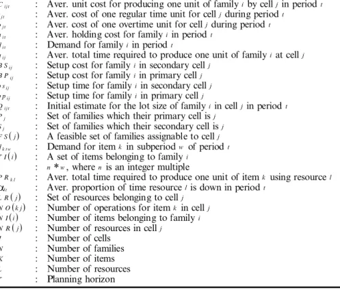
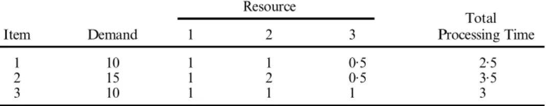
Our aim is to allocate production capacity among GT families and items by means of the proposed aggregate planning model. This can be achieved by solving a multi-period optimization problem which minimizes the summation of production, setup, inventory holding, and regular and overtime capacity costs subject to produc-tion and inventory balance constraints for families and items, and capacity feasibility constraints for GT cells and resources over the planning horizon. The objective function corresponds to the minimization of the variable cost of production. The set of the parameters and decision variables are given in tables 1 and 2, respectively. In the proposed cell loading approach we consider the capacity constraints at a more detailed level at the higher levels of the decision making hierarchy. As stated earlier, most of the hierarchical approaches in the literature either assume in® nite production capacity or deal with the capacity issues in an aggregated manner at the higher decision making levels, which might lead to an infeasible solution when we consider the detailed capacity constraints of bottleneck resources. Let’s look at the

following example of 3 items and 3 resources with the corresponding demand and processing times per item on each resource as shown in table 3. If we assume that the available capacity for each resource is 40 time units then total available capacity is 40

_*

3= 120 time units, and total required capacity is 2.5

_*

10+ 3.5

_*

15+ 3

_*

10 = 107.5 time units. If we only apply an aggregated capacity check then we conclude that there is enough capacity so we proceed on. Although we cannot meet total demand requirements by producing exactly the required quantities at the required period with zero inventories since Resource 2 is a bottleneck resource and 1

_*

10+ 2

_*

15+ 1

_*

10= 50

>

40.

An A/D scheme is applied to reduce the size of the problem, where the decom-position of the manufacturing system proceeds in three dimensions: by ¯ oor space

Cijt : Aver. unit cost for producing one unit of familyi by celljin periodt

rjt : Aver. cost of one regular time unit for celljduring periodt

ojt : Aver. cost of one overtime unit for cellj during periodt

hit : Aver. holding cost for familyiin periodt

dit : Demand for familyiin periodt

aij : Aver. total time required to produce one unit of familyiat cellj

B Sij : Setup cost for familyiin secondary cellj

B Pij : Setup cost for familyiin primary cellj

b sij : Setup time for familyiin secondary cellj

b pij : Setup time for familyiin primary cellj

Qijt : Initial estimate for the lot size of familyiin cellj in periodt

Pj : Set of families which their primary cell isj

Sj : Set of families which their secondary cell isj

F S(j) : A feasible set of families assignable to cellj dk tw : Demand for itemk in subperiodw of periodt

T I(i) : A set of items belonging to familyi

t : n*w, wheren is an integer multiple

P Rk l : Aver. total time required to produce one unit of itemk using resourcel

a lt : Aver. proportion of time resourcelis down in periodt

L R(j) : Set of resources belonging to cellj N O(k j) : Number of operations for itemk in cellj N I(i) : Number of items belonging to familyi N R(j) : Number of resources in cellj

J : Number of cells N : Number of families K : Number of items L : Number of resources T : Planning horizon Table 1. Parameters.

Xijt : Number of units of familyiproduced by cellj in periodt

I Fit : Inventory of familyiat the end of periodt

Ojt : Overtime used by celljin periodt

Rjt : Regular time used by celljin periodt

Zk jt w : Number of units of itemk produced by celljin subperiodw of periodt

Ik t w : Inventory of itemk at the end of subperiodw of periodt

O Rlt : Overtime used by resourcelin periodt

R Rlt : Regular time used by resourcel in periodt Table 2. Decision variables.

(or resource-based

)

, by product, and by time horizon. In the ¯ oor space decomposi-tion, the manufacturing system is divided into a set of GT cells where each cell is designed to produce a GT family or families. In the product-based decomposition, similar items are grouped into GT families, based on their designs or processes, or both. Throughout this research a GT family is de® ned as a set of items that require similar machinery, tooling, machine operations, jigs and ® xtures. Both GT cell for-mation and the prerequisite product family determinations are assumed to have been done a priori to this planning activity, but their impact on the performance of the results are tested in § 4. In the time scale decomposition, the levels of the decision hierarchy di€ er by complexity, scope and time horizon in that higher levels deal with longer range and more aggregated issues, and lower levels deal with short term and more speci® c issues. The linkage between the di€ erent levels is achieved through a feedback mechanism and a set of Lagrange multipliers as discussed in the next section. Our time scale decomposition corresponds to the shop and cell levels of the control structure developed for the automated manufacturing research facility at the National Institute of Standards and Technology in the USA, which decomposes the manufacturing functions into ® ve levels: facility, shop, cell, workstation, and equipment as discussed by Jackson and Jones (1987

)

.

A mathematical formulation of the problem is as follows: Minimize

å

T t=1

å

J j=1

(

iÎ

å

FS(j) Cijt

´

Xijt+

å

iÎ Sj (BSij/Qijt)

´

Xijt+

å

iÎ Pj (BPij/Qijt)

´

Xijt + ojt

´

Ojt+ rjt

´

Rjt

)

+

å

T t=1

å

N i=1 hit

´

IFit subject to

•

production and inventory balance equations for each family:

å

_j=1J Xijt+ IFi,t-1

-

IFit= dit, for i= 1

,

. . .

,

N and t= 1

,

. . .

,

T (1)

•

capacity restrictions for each cell:

å

iÎ FS(j) aij

´

Xijt+

å

iÎ Sj (bsij/Qijt)

´

Xijt+

å

iÎ Pj (bpij/Qijt)

´

Xijt

-

Ojt = Rjt for j= 1

,

. . .

,

J and t= 1

,

. . .

,

T (2) Resource

Item Demand 1 2 3 Processing Time

1 10 1 1 0.5 2.5

2 15 1 2 0.5 3.5

3 10 1 1 1 3

Table 3. Aggregate capacity planning problem.

Total

0

£

Ojt

£

(Upper limit

)

"

j and t (3)

0

£

Rjt

£

(Upper limit

)

"

j and t (4)

•

production and inventory balance equations for each item:

å

_j=1J Zkjtw+ Ikt,w-1

-

Iktw= dktw

"

k

Î

TI(i)

,

w and t (5)

•

inventory consistency equations:

å

kÎ TI(i)

å

n w=1

Iktw

-

IFit= 0

"

i and t (6)

•

capacity restrictions for each resource:

å

iÎ FS(j)kÎ

å

TI(i) PRkl

å

n w=1 Zkjtw

(

)

-

ORlt= RRlt

"

l

Î

L R(j)

,

j and t (7)

0

£

ORlt

£

(Upper Limit

)

"

l and t (8)

0

£

RRlt

£

(Upper limit

)

´

( 1

-

a

lt)

"

l and t (9)

•

resource consistency relations:

å

lÎ L R(j) ORlt

-

Ojt= 0

"

j and t (10)

å

lÎ L R(j) RRlt

-

Rjt= 0

"

j and t (11)

•

non-negativity restrictions:

Xijt

,

IFit

,

Ojt

,

Rjt

,

Zkjtw

,

Iktw

,

ORlt and RRlt

³

0

"

i

,

j

,

k

,

l

,

t and w. (12)

The constraint sets (1

)

and (5

)

are the inventory balance constraints for families and items, respectively, in which both the amount of inventory left in stock at the end of each period and the demand in each period are supplied by the amount of production in each period and the amount of inventory carried over from the pre-vious period. No backordering is allowed. Moreover, a deterministic, but time-vary-ing, demand for every item in every time period is assumed. Constraint (6

)

, which represents the inventory consistency equations, links the item inventories to the inventory of the associated family. This constraint requires that the inventory for a family equal to the sum of the inventories of the items contained in the family. As a result, individual items are mapped into their corresponding families. Given that

å

n

w=1

å

kÎ TI(i)dktw= dit, it can be shown that the constraint set, which includes

all the resource, production and inventory constraints, implies that

å

n

w=1

å

kÎ TI(i)Zkjtw = Xijt for all i, j and t; that is, for each time period total

family production equals the sum of the production quantities for its items. Constraints (2

)

and (7

)

are the capacity feasibility constraints for GT cells and resources. Upper limits on regular and overtime usages are also de® ned by con-straints (3

)

, (4

)

, (8

)

and (9

)

. For the computational analysis, the upper limits on the overtime are set to 25% of the upper limits on the amount of regular time available. Constraints (10

)

and (11

)

link the available time for each GT cell to the

resources comprising that cell. An important assumption concerns the de® nition of the capacity, which depends on the time scale. Long-term capacity is a statistical average of actual short-term capacity. The available resource times are de® ned in terms of proportion of time down, such as if a resource is down 10% of the time, and this will be deducted from its available capacity as shown in constraint (9

)

. As a result, the production quantities are determined such that they are much more likely to be within the current capacity of the system as prescribed by chance constrained programming in Charnes and Cooper (1959

)

.

Implicit in constraint (2

)

is the possibility that each GT family can have more than one feasible cell for its production. A feasible cell is de® ned as a cell in which a family can be processed entirely within that cell considering feasibility requirements. A more detailed discussion on the formation of primary and secondary cells can be found in Akturk and Balkose (1996

)

. It is assumed that the primary cell of a family is capable of producing the family at the lowest possible cost. Secondary cells are the ones in which the manufacture of the family is possible at a higher cost, due to both increased setup and material handling costs, assuming that all cells are initially tooled for their primary families. An additional cost is incurred when other than the primary families need to be produced at that cell. Therefore, the setup costs and setup times for the families in their secondary cells are assumed greater than the setup costs and setup times in the primary cells. The parameter, Qijt, is an initial

estimate for lot size allowing the cell resource constraints to approximately account for the total setup time which is directly proportional to the number of setups required to meet the desired production quantities at each cell. Also, the de® nition of primary and secondary cells for each family allows the production management system to react to the variations in the families’ total demand. For example, during a very low demand period, one cell may be completely shut down because of main-tenance and that cell’s families are assigned to some other cell.

At the cell loading level, there are three basic ways of responding to changes in demand: holding a relatively constant production rate and using inventory to satisfy demand peaks, using changes in level of production to follow demand closely, or combining these two strategies to meet demand. There are di€ erent ways to change the level of production, including overtime and assigning some of the items into their secondary cells with an additional production cost and time. Given a capacity limit, tradeo€ s can be made among the costs of inventory, overtime and secondary cells. To further illustrate the mathematical formulation of the cell loading problem, we consider a numerical example involving 4 GT families and 2 manufacturing cells such that P1=

{

Family 1

,

2

}

, P2=

{

Family 3

,

4

}

, S1=

{

Family 3

}

and

S2=

{

Family 1

}

, consequently FS(1) =

{

1

,

2

,

3

}

and FS(2) =

{

1

,

3

,

4

}

. The

plan-ning horizon consists of 4 periods. Furthermore, there are 20 items and 9 resources, and their corresponding families and cells, respectively, are as follows:

TI(1) =

{

Item 1

,

2

,

3

,

4

,

5

,

6

}

, TI(2) =

{

Item 7

,

8

,

9

,

10

,

11

}

, TI(3) =

{

Item 12

,

13

,

14

,

15

,

16

}

, TI(4)=

{

Item 17

,

18

,

19

,

20

}

, L R(1)=

{

Resource 1

,

2

,

3

,

4

,

5

}

, and

L R(2) =

{

Resource 6

,

7

,

8

,

9

}

. The cost parameters are C1,1,t = 0.75, C1,2,t= 1.49,

C2,1,t = 1.11, C3,1,t= 1.88, C3,2,t = 1.13, C4,2,t= 0.92, r1,t = 0.58, r2,t= 1.17,

ojt= 2

*

rjt, and hit=(1+ 0.05(t

-

1))

*

UN~

[

1.5

,

2.5

]

for every t

Î

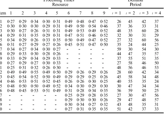
T . The

corre-sponding data for each item are given in table 4.

We have created two scenarios. In the ® rst scenario, RRlt

£

120 and ORlt

£

30

for every l and t. The optimal solution for the cell loading problem is summarized in table 5. In order to simplify the output, we only present the results for families and

cells. In this solution, all of the items are assigned to their primary cells, and both overtime and inventory options are utilized to absorb the demand changes. The objective function value is equal to 6654.6. In the second scenario, we decreased the available resource capacities in cell 1 to RRlt

£

80 and ORlt

£

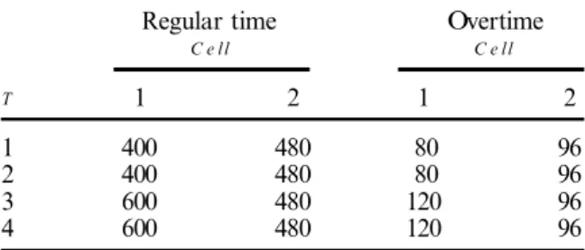
16 for the ® rst two

periods. The upper limits on the resource availabilities in each cell are given in table 6. In this case, some of the items of Family 1 are assigned to their secondary cells, i.e. Cell 2, in addition to the overtime and inventory options as shown in table 7. As a result of that the objective function value is increased to 6861.4.

3. S olution procedure

Linear programming (LP

)

is a convenient type of model to use at this level because of the wide availability of LP codes. LP also permits sensitivity and parametric

Processing Times Demand

Resource Period Item 1 2 3 4 5 6 7 8 9 t=1 t= 2 t=3 t =4 1 0.27 0.29 0.34 0.30 0.31 0.49 0.48 0.47 0.52 26 45 42 37 2 0.30 0.30 0.30 0.29 0.31 0.49 0.50 0.54 0.46 37 36 33 31 3 0.30 0.27 0.26 0.31 0.31 0.49 0.53 0.49 0.52 48 35 60 28 4 0.29 0.31 0.35 0.29 0.31 0.47 0.51 0.46 0.52 32 30 31 29 5 0.34 0.29 0.26 0.33 0.35 0.50 0.49 0.47 0.52 27 32 60 56 6 0.31 0.27 0.29 0.27 0.26 0.45 0.51 0.47 0.50 35 24 44 25 7 0.34 0.27 0.34 0.30 0.27

-

-

-

-

59 30 54 30 8 0.29 0.33 0.30 0.28 0.26

-

-

-

-

44 47 35 57 9 0.33 0.29 0.34 0.29 0.33

-

-

-

-

37 55 51 35 10 0.27 0.29 0.27 0.30 0.33

-

-

-

-

27 58 46 50 11 0.25 0.31 0.32 0.26 0.30

-

-

-

-

48 56 46 53 12 0.49 0.49 0.55 0.49 0.50 0.29 0.26 0.29 0.26 28 60 42 34 13 0.45 0.54 0.52 0.50 0.49 0.29 0.29 0.25 0.26 45 58 34 48 14 0.46 0.53 0.51 0.52 0.45 0.26 0.26 0.30 0.25 40 55 35 24 15 0.48 0.50 0.50 0.49 0.52 0.34 0.30 0.29 0.30 30 47 34 34 16 0.48 0.45 0.53 0.51 0.49 0.31 0.28 0.34 0.35 56 59 50 25 17

-

-

-

-

-

0.25 0.29 0.28 0.35 27 30 47 56 18

-

-

-

-

-

0.29 0.30 0.30 0.26 29 47 48 57 19

-

-

-

-

-

0.30 0.34 0.27 0.32 43 48 35 31 20

-

-

-

-

-

0.27 0.31 0.35 0.35 51 42 37 33

Table 4. Item data for numerical example.

Regular time Overtime Inventory Number of units produced

Cell Cell Family Family

1 2 3 4

T 1 2 1 2 1 2 3 4 cell 1 cell 1 cell 2 cell 2

1 514.2 386.4 0 0 0 19 0 0 205 234 199 150

2 545.0 479.6 0 13.25 37 0 0 0 239 227 279 167

3 544.0 401.3 0 0 0 0 0 0 233 232 195 165

4 504.7 379.9 0 0 0 0 0 0 206 225 165 177

Table 5. Optimal solution for scenario.

analysis to be performed quite easily and the information on dual values can be derived at little additional computational cost. It is also important to consider how such a production planning system would be implemented in practice. The planning horizon given by the mathematical model is posed as if all demand is known with certainty and all parameters are to be frozen over the planning horizon. Because of the uncertainties present in the planning process, a rolling horizon method with a lookahead mechanism similar to Maes and Van Wassenhowe (1986

)

is applied to solve this model in each period in order to deal with either ¯ uctuations or season-alities in demand or other inputs. The lookahead mechanism anticipates possible capacity shortages and considers the following tradeo€ s to minimize the variable production cost: building up su cient inventory in earlier periods by increasing production rates, or using overtime, or assigning families to their secondary cells with an additional cost of production, or a mixture of these alternatives. Baker (1977

)

describes, `the typical scenario of a rolling horizon procedure is as follows: solve the model and implement only the ® rst period’s decisions; for the following period, update the model to re¯ ect information collected in the interim, re-solve the model, and implement only the imminent decision pending subsequent model runs’. That is, the implementation of rolling horizons requires routinely updating or revis-ing plans takrevis-ing into consideration more reliable data as they become available. The rolling horizon procedure simply re¯ ects the continuity of the production planning and scheduling process into a non-® nite future.

The size of the problem is an important issue for LP applications, because the time required to ® nd an optimum solution increases with the number of constraints.

Regular time Overtime

C e ll C e ll T 1 2 1 2 1 400 480 80 96 2 400 480 80 96 3 600 480 120 96 4 600 480 120 96

Table 6. Upper limits on reesource availabilities for scenario 2

Regular time Overtime Inventory Number of units produced

Cell Cell Family Family

1 2 3 4

T 1 2 1 2 1 2 3 4 cell 1 cell 2 cell 1 cell 1 cell 2 cell 2

1 400 478.6 76.7 0.0 0 0 62 0 192 13 215

-

261 150

2 400 480 79.0 20.8 0 0 0 0 162 40 246

-

217 167

3 586.6 401.3 0 0 0 0 0 0 270

-

232

-

195 167

4 504.7 379.9 0 0 0 0 0 0 206

-

225

-

165 177

Table 7. Optimal solution for scenario 2.

On the other hand, recent advancements in microelectronics are making multipro-cessor systems more cost-e€ ective than a single promultipro-cessor. Distributing a task over a multiprocessor (or parallel

)

system can increase system throughput and speed up computation. Decomposition methods allow large scale models to be broken down into manageable sub-models, and then systematically reassembled. These methods show considerable promise for time critical decision support applications, especially when the methods have been adapted for and implemented on parallel computers. Decomposition methods can be ine cient on serial computers when compared to a monolithic approach, unless the subproblems have a special structure that may be exploited.

The optimization of decomposable problems comprised of a number of related subproblems is an important and frequently referred to topic in the literature with an early seminal discussion given by Geo€ rion (1970

)

. The two principal types of decomposition methods that have appeared in the literature are price directed decomposition and resource directed decomposition. In price directed decomposi-tion, the separation is accomplished by putting prices, or dual variables, on the joint constraints and placing them in the objective function. The price directed coordina-tion problem is concerned with calculating optimal prices on the shared resources to be used in the subproblems so that an optimal solution to the overall problem is achieved by optimizing separately each of the subproblems. In resource directed decomposition, each of the subproblems is given a portion of the shared resources. The resource directed coordination problem is concerned with e€ ecting an appor-tionment that permits the overall problem to be optimized by optimizing separately each of the subproblems. Both types of decomposition are aimed at decomposing the overall problem into, essentially, k separate optimization problems. Making a choice between price and resource directed decomposition is based on which approach leads to a set of subproblems with the most exploitable structure. A discussion on the di€ erent decomposition principles is given in detail in Geo€ rion (1970

)

and Shapiro (1993

)

.

The solution procedure proposed for the cell loading problem is an example of a price directed decomposition. It consists of formulating a Lagrangean relaxation of the initial model and solving this dual problem by an e cient, iterative solution procedure. For the problem given in the previous section, the joint constraints, or coupling constraints, which are inventory (6

)

, and resource consistency (10

)

and (11

)

equations, are dualized to obtain:

L(¸

,

¹1

,

¹2) = Minimize

å

T t=1

å

J j=1

(

iÎ

å

FS(j) Cijt

´

Xijt+

å

iÎ Sj (BSij/Qijt)

´

Xijt +

å

iÎ Pj (BPij/Qijt)

´

Xijt+ ojt

´

Ojt+ rjt

´

Rjt

)

+

å

T t=1

å

N i=1 hit

´

IFit+

å

n i=1

å

T t=1 ¸it

å

kÎ TI(i)

å

n w=1 Iktw

-

IFit

æ

è

ö

ø

+

å

J j=1

å

T t=1 ¹1_jt

å

lÎ L R(j) ORlt

-

Ojt

æ

è

ö

ø

+

å

J j=1

å

T t=1 ¹2_jt

å

lÎ L R(j) RRlt

-

Rjt

æ

è

ö

ø

subject to constraint sets 1, 2, 3, 4, 5, 7, 8 and 9. The dual problem to the original problem is:

(D) max

¸,¹1,¹2L

(¸

,

¹1

,

¹2)

Furthermore, the Lagrangean relaxation as given above may be separated into the following two subproblems:

•

family/cell aggregation subproblem (FCA

)

Minimize

å

T t=1

å

J j=1

(

iÎ

å

FS(j) Cijt

´

Xijt+

å

iÎ Sj (BSij/Qijt)

´

Xijt+

å

iÎ Pj (BPij/Qijt)

´

Xijt +(ojt

-

¹1jt)Ojt+(rjt

-

¹2jt)Rjt

)

+

å

T t=1

å

N i=1 (hit

-

¸it) IFit

subject to constraint sets 1, 2, 3 and 4.

•

Item/resource disaggregation subproblem for each t (IRDt

)

Minimize¸it

å

kÎ TI(i)

å

n w=1 Iktw

æ

è

ö

ø

+¹1jt

å

lÎ L R(j) ORlt

æ

è

ö

ø

+¹2jt

å

lÎ L R(j) RRlt

æ

è

ö

ø

subject to constraint sets 5, 7, 8 and 9.

The IRDt model is solved over a shorter horizon, t, with periods, w, allowing a

® ner resolution than period t used for the subproblem FCA. For instance, items might be scheduled weekly, while the production of families would be planned monthly. The linkage mechanism for these two subproblems is resource and inven-tory consistency relationships which are priced out by a set of Lagrange multipliers

¸,¹1and¹2, which re¯ ect the cost penalties at the item level due to the requirements

set at the family level. The determination of these multipliers provides a feedback process in the hierarchical framework. Furthermore, the separation of the mathe-matical formulation into the FCA and IRDt subproblems allows us to solve these

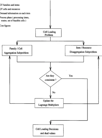
optimization problems in parallel as shown in ® gure 1.

The dual problem is to ® nd¸, ¹1 and¹2 to maximize the Lagrangean as stated

above. For a primal-dual approach to solving the Lagrangean, the Lagrangean is solved for a given¸,¹1and¹2, and based on this solution a new set of multipliers is

calculated. Recognizing that¸, ¹1and¹2 may be interpreted as the marginal cost of

having to provide additional increments of inventory, overtime and regular time in time period t, this iterative process continues until the inventory and resource con-sistency relationships are satis® ed within an e range of the best known feasible

solution. The revision of the multipliers depends upon the current degree of incon-sistency between the FCA and IRDt subproblems. A subgradient optimization

method, similar to Held et al. (1974

)

, is used to update the values of Lagrange multipliers. A validation of the subgradient optimization method can be found in Held et al. (1974

)

. The¸it values at step c are updated by the formula:

¸cit+1=¸cit+d c

å

kÎ TI(i)

å

n w=1 Iktw

-

IFit

æ

è

ö

ø

.

whered cis a positive scalar step size which is determined by the following formula:

d c= q c(Z

*

_-

_L(¸

_,

_¹1

,

¹2))

(

_kÎ

å

_TI(i)w

å

n₌₁Iktw

-

IFit

)

2.

In this formula, Z*is the objective function of the best known feasible solution to the original problem, which provides an upper bound on the dual problem, andq cis a

scalar between 0 and 2. A description of an upper bounding heuristic is given in the Appendix. The sequence of q c is determined by setting q 0, initially to 0.01 and

increasing by a factor of two whenever the Lagrangean dual has failed to increase in a speci® c number of iterations. Fisher (1985

)

has shown empirically that this rule

Figure 1. Flow-chart representation of the algorithm’s framework.

works well, although it is not guaranteed to satisfy the complementary slackness condition for convergence.

4. Computational analysis

The proposed cell loading algorithm and the matrix generator for the problem formulation are coded in the C language. An optimal solution is found by using the CPLEX optimization package on a Sparcstation 10 under SunOS 5.4. We wish to investigate to what degree the proposed approach is robust in the face of uncertainty and how sensitive it is to the assumptions we have made throughout this research with regard to machine-component groupings, GT cells and families, inclusion of new products to the existing families, and resource availabilities. There are a large number of variables which could have an e€ ect on the performance of the cell loading problem. Within the conceptual framework of the hierarchical procedure, an experimental design is developed with two objectives in mind. The ® rst objective is to generate a set of test problems to calculate the computation time to ® nd an optimal solution. The second objective is to explain the relationships between the variable production cost and the system parameters.

There are ® ve experimental factors that can a€ ect the e ciency of the proposed approach, which are listed in table 8. The initial estimation of lot sizes depends on the direct setup cost for each item, and plays an important role within the context of the trade-o€ s between inventory holding and overtime costs since it determines the number of setups required. The direct setup cost, to make the results of the research meaningful, must be compared to the inventory holding cost as a ratio, S/I, as suggested by Maes and Van Wassenhowe (1986

)

. The S/I ratios, factor A, are used to ® nd the initial lot size of family i in cell j in period t as

Qijt=

Ï

ê ê ê ê ê ê ê ê ê ê ê ê ê ê ê ê ê ê ê ê ê ê ê ê ê ê ê ê ê ê êê2

´

S/I ratio

´

dit for every i

Î

FS(j). The representative ranges for factor

B, the number of families, and factor D, the number of cells, are based on the studies done by Hyer and WemmerlÈov (1989

)

, and WemmerloÈv and Hyer (1989

)

on current practices seen in industry for GT and CM systems. In addition, an assignment of the items to the GT families is one of the objectives of the part-family and machine-cell formation problem. These assignments are done depending upon the similarities that exist between the items, and similarity coe cients are calculated using several criteria as discussed in Shafer and Rogers (1993

)

and O€ odile et al. (1994

)

. Factor E, the number of items in each family, re¯ ects the fact that the variability within each family could be di€ erent depending upon the threshold values used to form the GT families. A high threshold value means a low feature variability and a high similarity among the items in each family. Since the total number of items is a ® xed parameter for all runs, factor E is used to measure the impact of variability in each family by varying the size of the each family, and the processing time for each

Factors De® nition Low High

A S/I ratio 0.75 1.25

B Number of families 15 35

C Upper limits on resource availability No idle time 10% idle time

D Number of GT cells 5 10

E Set of items within each family Low variability High variability

Table 8. Experimental factors.

item k on resource l, PRkl, is based upon the degree of similarity in each family, as

can be seen in table 9. The levels of factor C specify the upper limits on resource availability where the low level corresponds to a congested shop ¯ oor, while the high level represents a 10% idle time. Since there are ® ve factors and two levels, our experiment is a 25 full-factorial design, which corresponds to thirty-two treatment combinations. The number of replications of each combination is taken as ® ve producing 160 di€ erent randomly generated runs.

Other variables in the system are treated as ® xed parameters and summarized in table 9, where UN~

[

a

,

b

]

represents a uniformly distributed random variable in interval

[

a

,

b

]

. All of the parameters’ values are constant throughout the planning horizon, except the inventory holding cost for family i in period t, hit, which increases

over time to approximately account for factors like in¯ ation and time value of money. Furthermore, there are some other parameters, such as dit and aij, that

assume ® xed parameter values. The e€ ective demand for each item in each subperiod of each period, dktw, is ® xed. Therefore, the demand for each family in a particular

period should be calculated by summing the demands of all of the items belonging to that family corresponding to that period; i.e.

dit =

å

n w=1kÎ

å

TI(i)

dktw

"

i

,

t

The processing time of each item at each feasible resource, PRkl, and the number of

operations for each item are ® xed. So, the average total time required to produce one unit of family i at cell j, aij, should be the product of the average processing time of

an item belonging to family i at cell j and the average number of operations required for an item k in family i. A mathematical expression is given below.

Parameters Set of values

Total number of items,K 250

Total number of resources,L 50

Number of periods,T 12

Number of subperiods per period 4

Cost of production,Cijt UN~[0.75, 1.25] if i

Î

Pj

UN~ [ 1.5, 2.0] ifi

Î

Sj

Cost of regular time,rj t UN~[1.25, 2.0]

Cost of overtime,ojt 2* rjt

Inventory holding cost,hit (1+0.05(t

-

1))*UN~

[

1.5

,

2.5

]

Setup cost for the families, BSij andB Pij 0.03*Cijt *dit

Processing times,P Rk l (1)Low variability UN~ [ 0.25, 0.35] if i

Î

Pj UN~ [ 0.45, 0.55] ifi

Î

Sj (2)High variability UN~ [0.2, 0.4] if i

Î

Pj UN~ [0.4, 0.6] ifi

Î

Sj Setup times (0.1_*aij) if i

Î

F S(j)

Number of operations per item UN~ [3, 5]

E€ ective demand,dk t w UN~ [6, 15]

Table 9. Fixed parameters.

aij=

(

_å

_{kÎ TI}(i)

å

lÎ L R(j) PRkl)(

å

kÎ TI(i) NO(kj))

NI(i)2

_´

_NR(j)

"

i

Î

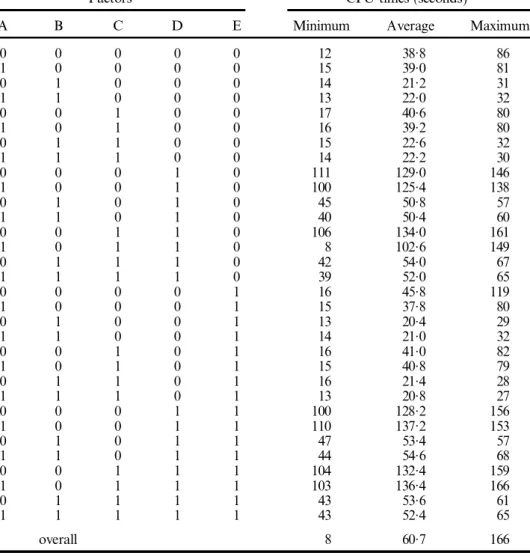
FS(j).

Table 10 summarizes the CPU times (in seconds

)

to ® nd the optimum solution for each run, along with the minimum, average, and maximum CPU times (based on ® ve random replications

)

for each factor combination. In this table, low and high levels for each factor are represented by 0 and 1, respectively. For all 160 problems reported in this table, the maximum CPU time was 166 s, whereas the average time was 60.7 s. The maximum CPU time was found for the factor combination of (1 0 1 1 1

)

. In other words, all the factors except the number of families were at their high levels. On the other hand, the minimum average computation time is found for the factor combination of (0 1 0 0 1

)

, where the S/I ratio, upper limit on the resource avail-ability and the number of GT cells were at their low levels. Furthermore, if we would like to use the Lagrangean relaxation procedure discussed in § 3 on a parallel

pro-Factors CPU times (seconds)

A B C D E Minimum Average Maximum

0 0 0 0 0 12 38.8 86 1 0 0 0 0 15 39.0 81 0 1 0 0 0 14 21.2 31 1 1 0 0 0 13 22.0 32 0 0 1 0 0 17 40.6 80 1 0 1 0 0 16 39.2 80 0 1 1 0 0 15 22.6 32 1 1 1 0 0 14 22.2 30 0 0 0 1 0 111 129.0 146 1 0 0 1 0 100 125.4 138 0 1 0 1 0 45 50.8 57 1 1 0 1 0 40 50.4 60 0 0 1 1 0 106 134.0 161 1 0 1 1 0 8 102.6 149 0 1 1 1 0 42 54.0 67 1 1 1 1 0 39 52.0 65 0 0 0 0 1 16 45.8 119 1 0 0 0 1 15 37.8 80 0 1 0 0 1 13 20.4 29 1 1 0 0 1 14 21.0 32 0 0 1 0 1 16 41.0 82 1 0 1 0 1 15 40.8 79 0 1 1 0 1 16 21.4 28 1 1 1 0 1 13 20.8 27 0 0 0 1 1 100 128.2 156 1 0 0 1 1 110 137.2 153 0 1 0 1 1 47 53.4 57 1 1 0 1 1 44 54.6 68 0 0 1 1 1 104 132.4 159 1 0 1 1 1 103 136.4 166 0 1 1 1 1 43 53.6 61 1 1 1 1 1 43 52.4 65 overall 8 60.7 166

Table 10. Results of the computational experiments.

cessor, then the Lagrange multipliers are updated by a subgradient optimization method, which requires a calculation of an upper bound for the cell loading problem. In table 11, we compare the average results of the upper bound with the average optimum solution for each replication along with the computation time to ® nd the optimum solution and the % deviations. The minimum % deviation was 0.000 006% for the factor combination of (1 0 1 1 0

)

, whereas the maximum one was 6.05% for the factor combination of (1 0 1 0 1

)

. As mentioned above, the average computation time to ® nd the optimum solution was 60.7 s, which indicated that within the scope of our experimental framework these problems can be solved optimally using a commercial optimization package on a serial processor without using a means of decomposition.

Finally, a two-way analysis of variance (ANOVA

)

test was applied to two per-formance measures, the optimum value of the total production cost and the compu-tation time, to test the equality of observed responses from the di€ erent treatment combinations of the chosen factors. The number of GT cells and families, factors D and B, respectively, were found to be signi® cant at the 0.1% signi® cance level on the computation time criterion, followed by the factor E, the number of items in each family, that was used to represent the variability of the items within each family. For the total production cost criterion, the factor D was the only signi® cant one at the 0.1% signi® cance level. The number of GT cells, factor D, is the most important output of classi® cation and coding systems (CCS

)

and cell formation techniques discussed in § 1. ANOVA tables indicated that the factor D has the most signi® cant e€ ect on both of the performance measures considered. Therefore, an interface between CCS and cell loading decisions becomes a critical issue in any GT based production planning approach. Unfortunately, most of the existing approaches do not consider parameters associated with the cell loading activities during the initial design stage.

Another important question is the sensitivity of cell loading decisions with respect to the inclusion of new products into the existing GT families. Our computa-tional experiments indicate that if there is more feature variability among the items in each family, there will, consequently, be more in-process inventories, which is not desirable. Therefore, if the feature variability of the items in each family is reduced then the in-process inventory levels will tend to be decreased. Welke and Overbeeke (1988

)

report their experiences at Deere & Co., and argue that GT families and cells are generally constructed and based on the products that are currently being man-ufactured. In order to maintain the existing GT cell formation valid for a long time,

Optimum

Replication Upper Bound Solution Comp. time % dev.

Rep. 1 210 773.7 208 101.8 73.88 1.33 Rep. 2 209 556.7 204 966.3 57.25 2.28 Rep. 3 234 940.4 230 446.8 53.81 1.95 Rep. 4 233 865.1 231 608.9 65.22 1.04 Rep. 5 237 990.6 233 384.2 53.13 2.11 Overall 225 425.3 221 701.6 60.66 1.68

Table 11. Comparison of computational results.

certain plans must be made so that new products can be designed to fully conform to the existing manufacturing cells, i.e. design for manufacturing. Therefore, the exist-ing GT database should be an in¯ uencexist-ing factor as to how the new parts will be designed and processed within a CM system.

5. Conclusions

In this research, an aggregate planning model of the cell loading problem for CM systems has been developed to minimize the variable production cost. The proposed approach has several advantages over models in the current literature on hierarchical planning and cell loading. First, the proposed approach allows more accurate por-trayal of the operation of CM systems by using the capacity constraints to assess the impact of the cell loading decisions on the lower levels. As a result, the production rates are determined such that they are much more likely to be within the current capacity of the system. Another advantage is the enhanced computational tractabil-ity which is achieved by incorporating and combining the advantages of a hierarch-ical planning, a CM shop con® guration, and decomposition principles including Lagrangean relaxation and its related pricing mechanism. An aggregation/disaggre-gation scheme with respect to products, resources, and time horizon is also included in the mathematical formulation. The determination of Lagrange multipliers, which re¯ ect the cost penalties at the item level due to requirements set at the family level, provides a feedback process within the cell loading problem to satisfy the inventory and resource consistency constraints. Furthermore, the ANOVA tables indicated that the number of GT cells and families had a signi® cant e€ ect both on the total production cost and the computation time to ® nd an optimum solution. Therefore, in future CCS, the feedback information from the cell loading level should provide a more signi® cant input to the GT part-family machine-cell formation in addition to the other commonly used factors, i.e. design and processing requirements.

Acknowledg ments

The authors would like to thank two anonymous referees for their helpful sug-gestions on improving the paper, and to the National Science Foundation for par-tially supporting this research under grant DMC-8605972.

Appendix: Calculation of the upper boun d

The overall aim of the upper bounding algorithm is to produce all the required items at their primary cells in the amounts that they are demanded in each time period. An algorithmic description of the proposed algorithm is given below.

Step 1. Equalize the production level of each item at its primary cell at a particular

period to its demand at that period such that Zkjtw = dktw

"

k

Î

TI(i) and i

Î

Pj.

Step 2. Calculate the regular time and overtime requirements for each of the

resources in each cell. Let

TRlt =

å

iÎ FS(j)kÎ

å

TI(i) 1.1

_*

PRkl

*

å

n w=1 Zkjtw

(

)

"

t

,

j and l

Î

L R(j).

If TRlt

£

ULlt then RRlt= TRlt and ORlt= 0. Otherwise, RRlt= ULlt and

ORlt = TRlt

-

ULlt, where ULlt is the upper limit on the availability of

regular time at resource l in period t.

Step 3. Equalize the amount of production for each item at its primary cell in a

particular period to the total demand for that family in that period such that

Xijt = dit=

å

kÎ TI(i)

å

n w=1

Zkjtw

"

t and i

Î

Pj.

Step 4. Calculate the regular time and overtime requirements at each cell. Let TCjt=

å

iÎ Pjaij

*

Xijt

"

j and t. If TCjt

£

ULjt then Rjt = TCjt and

Ojt= 0. Otherwise, Rjt= ULjt and Ojt= TCjt

-

ULjt, where ULjt is the

upper limit on the availability of regular time in cell j in period t.

Step 5. Calculate the upper bound as follows: UB=

å

T t=1

å

J j=1

å

iÎ Pj

(Cijt+ BPij/Qijt)

´

Xijt+ ojt

´

Ojt+ rjt

´

Rjt

æ

è

ö

ø

+

å

T t=1

å

N i=1 hit

´

IFit.

The upper bounding algorithm utilizes the just-in-time logic in which the overall goal is to produce exactly the required quantities at precisely at the required period with zero inventories. The upper bound on the total production cost, which is based on the local information in each period, will tend to be larger than the optimum cost for the overall planning horizon when there is a high variability in demand and resource availabilities in the planning horizon as shown in table 11.

References

Akturk, M. S., andBalkose, H. O.,1996, Part-machine grouping using a multi-objective cluster analysis. International Journal of Production Research,34(8), 2299± 2315. Baker, K. R.,1977, An experimental study of the e€ ectiveness of rolling schedules in

produc-tion planning. Decision Sciences,8(1), 19± 27.

Bitran, G. R., Haas, E. A., and Hax, A. C.,1981, Hierarchical production planning: A single stage system. Operations Research,29, 717-743.

Bitran, G. R., andTirupati, D.,1993, Hierarchical production planning. In Handbooks in

Operations Research and Management Science,4, S. C. Graves, A. H. G. Rinnooy Kan,

and P. H. Zipkin (eds)(New York: Elsevier Science).

Charnes, A., and Cooper, W. W.,1959, Chance constrained programming. Management

Science,6, 73± 79.

Fisher, M. L.,1985, An applications oriented guide to Lagrangean relaxation. Interfaces,15

(2), 10± 21.

Geoffrion, A. M.,1970, Primal resource-directive approaches for optimizing nonlinear decomposable problems. Operations Research,18(3), 373± 403.

Graves, S. C.,1982, Using Lagrangean techniques to solve hierarchical production planning problems. Management Science,28(3), 260± 275.

Gunasekaran, A., Goyal, S. K., Virtanen, I., and Yli-Olli, P.,1994, An investigation into the application of group technology in advanced manufacturing systems.

International Journal of Computer Integrated Manufacturing,7(4), 215± 228.

Ham, I., Hitomi, K., andYashida, T.,1985, Group Technology Applications to Production

Management (Boston, MA: Kluwer-Nijho€).

Hax, A. C., and Meal, H. C.,1975, Hierarchical integration of production planning and scheduling. In Studies in Management Science, Vol. 1, L ogistics, M. A. Geisler (ed)

(Amsterdam: North-Holland).

Held, M., Wolfe, P., and Crowder, H. P.,1974, Validation of subgradient optimization.

Mathematical Programming, 6, 62± 88.

Hyer, N. L., andWemmerloïv, U.,1989, Group technology in the US manufacturing indus-try: A survey of current practices. International Journal of Production Research,27(2),

1287± 1304.

Jackson, R. H. F., andJones, A. W. T.,1987, An architecture for decision making in the factory of the future. Interfaces,17(6), 15± 20.

Maes, J., andVan Wassenhowe, L. N.,1986, Multi item single level capacitated dynamic lotsizing heuristics: a computational comparison (Part II: Rolling horizon). IIE

Transactions, 18(2), 124± 129.

McKay, K. N., Safayeni, F. R., and Buz acott, J. A., 1995, A review of hierarchical production planning and its applicability for modern manufacturing. Production

Planning and Control, 6(5), 384± 394.

Morris, J. S., and Tersine R. J.,1989, A comparison of cell loading practices in group technology. Journal of Manufacturing and Operations Management,2, 299± 313. Morris, J. S., andTersine R. J.,1990, A simulation analysis of factors in¯ uencing

attrac-tiveness of group technology cellular layouts. Management Science,36(12), 1567± 1578. Offodile, O. F., Mehrez A., andGrz nar, J.,1994, Cellular manufacturing: A taxonomic

review framework. Journal of Manufacturing Systems,13(3), 196± 220.

Shafer, S. M., andCharnes, J. M.,1995, A simulation analyses of factors in¯ uencing loading practices in cellular manufacturing. International Journal of Production Research,33(1),

279± 290.

Shafer, S. M., and Rogers, D. F., 1993, Similarity and distance measures for cellular manufacturing. Part II. An extension and comparison. International Journal of

Production Research, 31(6), 1315± 1326.

Shapiro, J. F.,1993, Mathematical programming models and methods for production plan-ning and scheduling. In Handbooks in Operations Research and Management Sciences, Vol. 4, S. C. Graves, A. H. G. Rinnooy Kan and P. H. Zipkin (eds)(New York: Elsevier Science).

Welke, H. A., and Overbeeke, J.,1988, Cellular manufacturing: A good technique for implementing just-in-time and total quality control. Industrial Engineering, 20, 11, 36±

41.

Wemmerloïv, U., andHyer, N. L.,1989, Cellular manufacturing in US industry: a survey of users. International Journal of Production Research, 27(9), 1511± 1530.