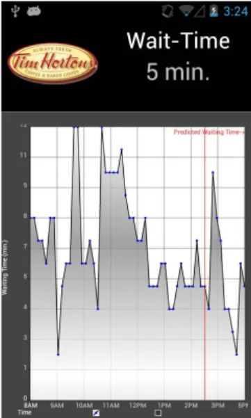
LineKing: Crowdsourced line wait-time estimation using smartphones
Tam metin
Şekil


Benzer Belgeler
When the spread between the interbank rate and depreciation rate of the local currency is taken as a policy tool, the empirical evidence suggests that the Turkish Central Bank
Methods: Patients who had recieved anakinra with a diagnosis of recur- rent pericarditis either idiopathic or secondary to FMF followed in our autoinflammatory disease center
Perceived usefulness and ease of use of the online shopping has reduced post purchase dissonance of the customers. Also, these dimensions are very strong and playing
Mehdi Bashiri, a third-year student at Istanbul Aydin University Dental Faculty, who received many medals from the most prestigious competitions in the world with his 21
The Effect Of Social Media Use To The Time Spent With Family Members, International Journal Of Eurasia Social Sciences, Vol: 9, Issue: 31, pp.. While these new
The performance of the ALE under different parameters such as the step size, filter length, and SNR has been studied extensively by simulations and experiments when
Hence, by variation of the wave function, we are able to represent the minimum tunneling time min (E) in terms of the transmission probability of the barrier and its set of
Blood samples were taken from the arterial line adding different discard volumes to the dead space.. Group names were given according to
