AN OBJECT RECOGNITION FRAMEWORK
USING CONTEXTUAL INTERACTIONS
AMONG OBJECTS
a thesis
submitted to the department of computer engineering
and the institute of engineering and science
of bilkent university
in partial fulfillment of the requirements
for the degree of
master of science
By
Fırat Kalaycılar
August, 2009
I certify that I have read this thesis and that in my opinion it is fully adequate, in scope and in quality, as a thesis for the degree of Master of Science.
Assist. Prof. Dr. Selim Aksoy(Advisor)
I certify that I have read this thesis and that in my opinion it is fully adequate, in scope and in quality, as a thesis for the degree of Master of Science.
Prof. Dr. Fato¸s T¨unay Yarman-Vural
I certify that I have read this thesis and that in my opinion it is fully adequate, in scope and in quality, as a thesis for the degree of Master of Science.
Assist. Prof. Dr. Pınar Duygulu-S¸ahin
Approved for the Institute of Engineering and Science:
Prof. Dr. Mehmet B. Baray Director of the Institute
ABSTRACT
AN OBJECT RECOGNITION FRAMEWORK USING
CONTEXTUAL INTERACTIONS AMONG OBJECTS
Fırat Kalaycılar
M.S. in Computer Engineering Supervisor: Assist. Prof. Dr. Selim Aksoy
August, 2009
Object recognition is one of the fundamental tasks in computer vision. The main endeavor in object recognition research is to devise techniques that make computers understand what they see as precise as human beings. The state of the art recognition methods utilize low-level image features (color, texture, etc.), interest points/regions, filter responses, etc. to find and identify objects in the scene. Although these work well for specific object classes, the results are not satisfactory enough to accept these techniques as universal solutions. Thus, the current trend is to make use of the context embedded in the scene. Context defines the rules for object - object and object - scene interactions. A scene configuration generated by some object recognizers can sometimes be inconsistent with the scene context. For example, observing a car in a kitchen is not likely in terms of the kitchen context. In this case, knowledge of kitchen can be used to correct this inconsistent recognition.
Motivated by the benefits of contextual information, we introduce an object recognition framework that utilizes contextual interactions between individually detected objects to improve the overall recognition performance. Our first con-tribution arises in the object detector design. We define three methods for object detection. Two of these methods, shape based and pixel classification based ob-ject detection, mainly use the techniques presented in the literature. However, we also describe another method called surface orientation based object detec-tion. The goal of this novel detection technique is to find objects whose shape, color and texture features are not discriminative while their surface orientations (horizontality or verticality) are consistent across different instances. Wall, table top, and road are typical examples for such objects. The second contribution is a probabilistic contextual interaction model for objects based on their spatial relationships. In order to represent the spatial relationships between objects,
iv
we propose three features that encode the relative position/location, scale and orientation of a given object pair. Using these features and our object inter-action likelihood model, we achieve to encode the semantic, spatial, and pose context of a scene concurrently. Our third main contribution is a contextual agreement maximization framework that assigns final labels to the detected ob-jects by maximizing a scene probability function that is defined jointly using both the individual object labels and their pairwise contextual interactions. The most consistent scene configuration is obtained by solving the maximization problem using linear optimization.
We performed experiments on the LabelMe [27] and Bilkent data sets by both utilizing and not utilizing the scene type (indoor or outdoor) information. While the average F2 score increased from 0.09 to 0.20 without the scene type assumption, it increased from 0.17 to 0.25 when the scene type is known on the LabelMe dataset. The results are similar for the experiments performed on the Bilkent data set. F2 score increased from 0.16 to 0.36 when the scene type information is not available and it increased from 0.31 to 0.44 when this additional information is used. It is clear that the incorporation of the contextual interactions improves the overall recognition performance.
¨
OZET
NESNELER ARASINDAK˙I BA ˘
GLAMSAL
ETK˙ILES
¸ ˙IMLER˙I KULLANAN B˙IR NESNE TANIMA
C
¸ ERC
¸ EVES˙I
Fırat Kalaycılar
Bilgisayar M¨uhendisli˘gi, Y¨uksek Lisans Tez Y¨oneticisi: Yard. Do¸c. Dr. Selim Aksoy
A˘gustos, 2009
Nesne tanıma, bilgisayarlı g¨orme alanının en temel problemlerinden biridir. Bilgisayarlar g¨ord¨uklerini insanlar gibi anlayabilsin diye teknikler geli¸stirmek nesne tanıma ara¸stırmalarındaki ana u˘gra¸stır. Bir sahnedeki nesneleri bul-mak ve tanımlayabilmek i¸cin en ¸cok kullanılan y¨ontemlerde, alt-d¨uzey g¨or¨unt¨u ¨
oznitelikleri (renk, doku, vb.), ilgi noktaları/b¨olgeleri, s¨uzge¸c tepkileri, vb. ¨
ozelliklerden yararlanılmaktadır. Bunlar belirli nesne sınıfları i¸cin d¨uzg¨un ¸calı¸ssa da, genel bir ¸c¨oz¨um olmaktan uzaktırlar. Bu y¨uzden, sahne ba˘glamını kullanmak g¨uncel bir e˘gilim halini almı¸stır. Ba˘glam nesneler arası ve nesne - sahne arası ili¸skilerin kurallarını belirlemektedir. Nesne tanıyıcıların ortaya ¸cıkardı˘gı sahne d¨uzenle¸simleri bazı durumlarda sahne ba˘glamıyla ¨ort¨u¸smemektedir. ¨Orne˘gin, bir mutfak ortamında araba g¨or¨ulmesi mutfak ba˘glamı a¸cısından pek olası de˘gildir. Bu durumda, mekanın bir mutfak oldu˘gunu bilmek bu t¨ur ¸celi¸skili tanımlamaları engellemekte kullanılabilir.
Ba˘glamsal bilginin getirdi˘gi faydaları hesaba katarak, bu tezde, nesne tanıma ba¸sarımını arttırmak i¸cin tek tek sezilmi¸s nesneler arasındaki ba˘glamsal et-kile¸simlerden yararlanan bir nesne tanıma ¸cer¸cevesi anlatılmaktadır. ˙Ilk katkımız nesne sezicilerin tasarımında g¨or¨ulmektedir. C¸ er¸cevemizde ¨u¸c farklı nesne sezim y¨ontemi tanımlanmı¸stır. Bunlardan ikisi, ¸sekil bazlı ve piksel sınıflandırması bazlı nesne sezicilerdir ve tasarımlarında genel olarak varolan y¨ontemlerden yarar-lanılmaktadır. Bunlardan ba¸ska, y¨uzey do˘grultusu bazlı nesne sezici isimli ¨u¸c¨unc¨u bir y¨ontem geli¸stirilmi¸stir. Bu yeni nesne sezim y¨ontemindeki ana ama¸c, ¸sekil, renk ve doku ¨ozellikleri ayırt edici olmasa da y¨uzey do˘grultuları (diklik ya da yataylık durumları) tutarlı olan nesnelerin sezilebilmesini sa˘glamaktır. Duvar,
vi
masa ¨ust¨u, yol, vb. nesneler bu gruba dahil edilmektedir. ˙Ikinci katkımız, nes-neler arasındaki uzamsal ili¸skilere dayanan ba˘glamsal etkile¸sim modelidir. Nes-neler arasındaki uzamsal ili¸skileri g¨ostermek i¸cin g¨oreli konum, ¨ol¸cek ve do˘grultu bilgilerini i¸ceren ¨u¸c tane ¨oznitelik tanımlanmı¸stır. Bu ¨oznitelikleri ve nesne etkile¸sim olurlu˘gu modelini kullanarak sahnenin anlamsal, uzamsal ve duru¸s ba˘glamları aynı anda ifade edilebilmektedir. ¨U¸c¨unc¨u ana katkımız, bireysel nesne etiketlerine ve nesne ikilileri arasındaki etkile¸simlere ba˘glı olan sahne olasılık fonksiyonunun enb¨uy¨ut¨ulerek, nesnelerin en son etiketlerinin atanmasıdır. En tutarlı sahne d¨uzenle¸simini bulmak i¸cin bu enb¨uy¨utme problemi, do˘grusal eni-yileme kullanılarak ¸c¨oz¨ulm¨u¸st¨ur.
LabelMe [27] ve Bilkent veri k¨umelerinde, hem sahne t¨ur¨un¨u (i¸c mekan ya da dı¸s mekan) hesaba katarak hem de katmayarak deneyler ger¸cekle¸stirilmi¸stir. LabelMe veri k¨umesinde sahne t¨ur¨u bilgisi kullanılmadı˘gında F2 ba¸sarı ¨ol¸c¨ut¨u 0.09’dan 0.20’ye y¨ukselmi¸stir. Sahne t¨ur¨u bilgisinden yararlanıldı˘gında F2 ¨ol¸c¨ut¨u 0.17’den 0.25 de˘gerine ula¸smı¸stır. Benzer ba¸sarım artı¸sları Bilkent veri k¨umesinde ger¸cekle¸stirilen deneylerde de g¨or¨ulm¨u¸st¨ur. Sahne t¨ur¨u hesaba katılmadı˘gında F2 ¨
ol¸c¨ut¨u 0.16’dan 0.36’ya y¨ukselirken, sahne t¨ur¨u dikkate alındı˘gında ¨ol¸c¨ut, 0.31 de˘gerinden 0.44 de˘gerine y¨ukselmi¸stir. Bu deneyler sonucunda, ba˘glamsal et-kile¸simlerin nesne tanıma ba¸sarımına olumlu bir etkisi oldu˘gu g¨osterilmi¸stir.
Acknowledgement
I would like to express my deep thanks to my advisor, Selim Aksoy, for his guidance and support throughout this work. It has been a valuable experience for me to work with him and get benefit from his vision and knowledge in every step of my research.
I am very thankful to Fato¸s T¨unay Yarman-Vural for inspiring me to choose computer vision as my research topic. If I had not met her at METU, I might have missed the chance to work on computer vision which now holds a great interest for me. In addition, I would like to thank her for the suggestions on improving this work.
I also would like to render thanks to Pınar Duygulu-S¸ahin for reviewing this thesis and providing useful feedback about the work presented here.
Certainly, I am grateful to my whole family for always being by my side. Without their endless support and caring, completion of this thesis would not be possible.
Aslı, Bahadır, C¸ aglar, Daniya, G¨okhan, Nazlı, Onur, Sare, Selen, Sıtar, Zeki and all other people I met at Bilkent made the last two years of my life very special and unforgettable. I cannot deny that their nice friendship and moral support helped me much in hard times.
Besides, I would like to express my pleasure on being part of Bilkent University and RETINA Group where I could always feel warmth and sincerity.
Finally, I would like to thank T ¨UB˙ITAK B˙IDEB (The Scientific and Techno-logical Research Council of Turkey) for their financial support.
To my family . . .
Contents
1 Introduction 1
1.1 Overview and Related Work . . . 1
1.2 Summary of Contributions . . . 8
1.3 Organization of the Thesis . . . 9
2 Object Detectors 11 2.1 Shape Based Object Detectors . . . 13
2.2 Pixel Classification Based Object Detectors . . . 17
2.3 Surface Orientation Based Object Detectors . . . 20
3 Interactions Between Scene Components 23 3.1 Spatial Relationship Features . . . 24
3.1.1 Oriented Overlaps Feature . . . 26
3.1.2 Oriented End Points Feature . . . 29
3.1.3 Horizontality Feature . . . 33
3.2 Object Interaction Likelihood . . . 34 ix
CONTENTS x
3.2.1 Spatial Relationship Feature Based Interaction Likelihood 35
3.2.2 Co-occurrence Based Interaction Likelihood . . . 39
4 Contextual Agreement Maximization 41 4.1 Scene Probability Function (SPF) . . . 41
4.2 Maximization of SPF . . . 43
4.3 Extendibility of the Model . . . 45
5 Experiments and Evaluation 48 5.1 Data Sets . . . 48
5.2 Object Detectors . . . 51
5.3 Experiments on the LabelMe Data Set . . . 52
5.4 Experiments on the Bilkent Data Set . . . 55
5.5 Results . . . 56
List of Figures
1.1 Example of object (coffee machine) - scene (kitchen) interaction [33]. 4 1.2 Similar object relationships in the 3D world can appear in many
different configurations in 2D images. . . 6
1.3 Overview of the contextual object recognition framework. . . 7
2.1 Sample detection mask. . . 12
2.2 Boosting based detection examples. . . 15
2.3 HOG based detection examples. . . 16
2.4 Pixel classification based object detection examples. . . 19
2.5 Surface orientation based detection examples. . . 22
3.1 Projection of an object onto the line with orientation θ. Blue re-gion: object to be projected, red line: orientation of projection, blue line segment: projected object. . . 25
LIST OF FIGURES xii
3.2 The computation of ρi,ref,θj. Here, the reference object, oref, is
shown as a blue region. The object whose oriented overlaps fea-ture is being computed, oi, is shown as a red-cyan region. The red
portion of oi is composed of the pixels whose projections are
val-ues in the [Zlref,θj, Zhref,θj] interval (the blue line segment). Thus, ρi,ref,θj is calculated as (number of oi’s red pixels)/(total number
of oi’s pixels). . . 27
3.3 Oriented overlaps feature space. While x-axis shows values of ρi,ref,0, y-axis corresponds to ρi,ref,90. Features are extracted for
the red object (oi) with respect to the green object (oref). See text
for more details. . . 28 3.4 An example computation of Ei,ref,θ. Here, the reference object,
oref, is shown as a blue region. The object whose oriented end
points feature is being computed, oi, is shown as a green region.
After the projection and normalization steps, the end points of the objects take the values shown in the figure. Thus, Ei,ref,θ is
computed as (−1.69, 0.28). . . 30 3.5 Oriented end points feature space for θ = 0. While x-axis shows
values of Γ(Zli,0), y-axis corresponds to Γ(Zhi,0). Features are ex-tracted for the red object (oi) with respect to the green object
(oref). See text for more details. . . 31
3.6 Oriented end points feature space for θ = 90. While x-axis shows values of Γ(Zl
i,90), y-axis corresponds to Γ(Zhi,90). Features are
ex-tracted for the red object (oi) with respect to the green object
(oref). See text for more details. . . 32
3.7 Example smoothed histograms extracted from the LabelMe data set. . . 37
LIST OF FIGURES xiii
5.2 Sample images from the Bilkent data set. . . 50 5.3 Average overall performance measurements for 5-fold cross
valida-tion applied on the LabelMe data set. The scene type assumpvalida-tion was not used. The settings are sorted in ascending order of the measure used. . . 57 5.4 Average overall performance measurements for 5-fold cross
valida-tion applied on the LabelMe data set under the scene type assump-tion. The settings are sorted in ascending order of the measure used. 58 5.5 Overall performance measurements for the experiments performed
on the Bilkent data set. The scene type assumption was not used. The settings are sorted in ascending order of the measure used. . . 59 5.6 Overall performance measurements for the experiments performed
on the Bilkent data set under the scene type assumption. The settings are sorted in ascending order of the measure used. . . 60 5.7 Sample final label assignments using the max, max/u, co and
OE90H (the best performing feature set) settings for an image from
the LabelMe data set. . . 67 5.8 Sample final label assignments using the max, max/u, co and
OE90H (the best performing feature set) settings for an image from
the LabelMe data set. . . 68 5.9 Sample final label assignments using the max, max/u, co and E0
(the best performing feature set) settings for an image from the Bilkent data set. . . 69 5.10 Sample final label assignments using the max, max/u, co and E0
(the best performing feature set) settings for an image from the Bilkent data set. . . 70
List of Tables
3.1 Properties of the spatial relationship feature histograms. . . 36
5.1 The groundtruth object counts in the LabelMe subset with 1975 images. . . 52 5.2 The groundtruth object counts in each LabelMe validation and
training data. Column V.i shows the number of the groundtruth objects for each class of interest (shown in the Class column) for the i’th validation data. Column T.i shows the number of the groundtruth objects for each class of interest for the i’th training data. . . 53 5.3 Experimental settings and their codes. . . 54 5.4 Categorization of 14 classes as indoor or outdoor object. . . 55 5.5 The groundtruth object counts in the Bilkent data set with 154
images. . . 55 5.6 Average F2 scores for each object class used in the experiments on
the LabelMe data set. These experiments were performed without using the scene type information. The italic values are the lowest of their rows and the bold ones are the highest. . . 64
LIST OF TABLES xv
5.7 Average F2 scores for each object class used in the experiments on the LabelMe data set. These experiments were performed using the scene type information. The italic values are the lowest of their rows and the bold ones are the highest. . . 64 5.8 F2 scores for each object class used in the experiments on the
Bilkent data set. These experiments were performed without using the scene type information. The italic values are the lowest of their rows and the bold ones are the highest. . . 65 5.9 F2 scores for each object class used in the experiments on the
Bilkent data set. These experiments were performed using the scene type information. The italic values are the lowest of their rows and the bold ones are the highest. . . 65
Chapter 1
Introduction
1.1
Overview and Related Work
Object recognition is one of the fundamental tasks in computer vision. It is defined as the identification of objects that are present in the scene. For a human being, recognition of objects is a straightforward action. This ability works well for the identification of objects in both videos and still images. The success in this task is not affected drastically even when the scene properties alter. For example, human vision system is nearly invariant to the changes in illumination conditions. Therefore, recognizing an object in a darker scene is not very much different than doing this in a brighter environment as long as the level of illumination is reasonable. Similarly, the occlusion of objects does not influence the recognition performance in a serious way. When the background clutter is considered, again human beings are good at disguishing an object from a complex background. Likewise, the different poses or visual diversity of objects do not have a significant effect on the recognition quality of the human vision system.
However, when a computer is programmed to mimic this seemingly simple ability of recognizing objects, unfortunately, the results are usually not satisfac-tory. Factors like illumination, occlusion conditions, background clutter, variety in pose and appearance are important challenges for computer vision. Thus, for
CHAPTER 1. INTRODUCTION 2
decades, vision scientists have been trying to develop algorithms to make com-puters understand what they see as precise as human beings.
There are different lines of research for the object recognition task. One of them is to decide if a member of an object class is present or absent in a given image regardless of its location. In [5, 8, 19], examples of this approach are described. The methods work well for images that contains a single object of interest and a relatively simple background. In this approach, first of all, some features (color, texture, etc.) and/or interest points (SIFT [21], Harris interest points [22] and etc.) are extracted. Then, decision on the existence of the object is made using the features and interest points.
The second line of research includes region-based methods that use segmen-tation to determine the boundaries of each object, and identify the objects by classifying these segments. An example work using this approach is explained in [3]. Although this method seems intuitive, it is often not possible to have a perfect segmentation. The most of the segmentation algorithms work well for scenes where objects have definite texture and color features. However, most of the objects are composed of parts with different properties so algorithms often segment these objects into several useless parts. To avoid this problem, multiple segmentation approaches have been used [13, 24, 26]. The idea behind multi-ple segmentations is that using different segmentation algorithms or running the same algorithms with different parameters may yield different segmentations of the image. Using the sets of pixels that are grouped into the same segments for different settings as consistency information, these methods try to decide on the most stable segmentation and use it for object recognition. Unfortunately, this approach usually works well when the number of objects in the scene is small.
The third line of research is direct detection where the input image is divided into overlapping tiles, and for each tile, the classifier decides if there is an object of a particular class or not [11, 28]. Alternatively, the detectors can make use of feature responses to determine the probable location of a target object [32]. After deciding on the tiles or the locations of target objects, detectors report the bounding boxes and the associated probabilities of existence. Another direct
CHAPTER 1. INTRODUCTION 3
detection method is part-based object recognition. In this method, first of all, discriminative parts of an object are detected. Then, using the individual parts and the part-based object model (relationship between the parts), the entire object can be captured. Example work using part-based object recognition can be found in [9, 10, 12].
None of these object recognition methods provides a universal methodology to solve the object recognition problem. The reason is that they do not make use of any high level information. They analyze the low level image features, filter responses, interest points, segmentations, etc. They do not take the structure and the constraints of the scene into account during the analysis. Actually, there is a rich source of high level information called context that can be used to enhance the recognition quality. Context refers to the rules and constraints of the object-object and object-scene interactions. Human vision and computer vision researchers [2, 15, 23] acknowledge that these contextual rules and constraints are useful while recognizing an object.
The literature on the visual perception [23] shows that context has influences at different levels. The semantic context represents the meaningfulness of the co-occurrences of particular objects. While table and chair have higher tendency to be found in the same scene, observing a car and a keyboard in the same environment is not likely. The spatial context puts constraints on the expected positions and locations of the objects. For instance, when a person sees an object flying in the sky, he knows that it is likely to be a bird or an airplane. The reason is that his cognitive system is aware that the probability of observing a flying tree, building, car, etc. is significantly low. In addition, the pose context defines the tendencies in the relative poses of the objects with respect to each other. For instance, we, human beings, anticipate that a car is oriented meaningfully on the road while driving.
Figure 1.1 shows an example emphasizing the importance of the contextual interactions [33] for human vision systems. When the whole scene is not visible, it is sometimes impossible to recognize the object of interest. But, recognition becomes easier when we see an object in the context of the scene it belongs to.
CHAPTER 1. INTRODUCTION 4
(a) Object (coffee machine) without scene con-text.
(b) Object (coffee machine) inside the scene (kitchen) context.
Figure 1.1: Example of object (coffee machine) - scene (kitchen) interaction [33]. In Figure 1.1(a), only the object of interest is shown. By just looking at that image, it is very hard to determine the type of the object. But, when it is known that it is a kitchen scene, it can be easily understood that it is a coffee machine as shown in Figure 1.1(b).
Motivated by the benefits of context for human visual perception, computer vision researchers devise techniques in which this rich information is incorporated into the entire recognition process. In [31], Torralba introduced a framework that models the relationship between the context and objects using the correlation between the statistics of the low-level features extracted from the whole scene and individual objects. In another work, Torralba et al. [33] proposed a context-based vision system in which global features are used in the scene prediction. The contextual information originating from that scene provides prior information for the local detectors. The main drawback of these approaches is that the scene context is modeled in terms of low-level features that may vary from image to image.
Besides the methods that deal with the correlations between low-level features, more intuitive models also exist. In [26], context in the scene is modeled in
CHAPTER 1. INTRODUCTION 5
terms of the co-occurrence likelihoods of objects (semantic context). An image is segmented into stable regions, and for each region, the class labels are sorted from the most to the least likely. By the help of the contextual model, the method manages to disambiguate each region and assigns a final class label. The main drawback of this method is its dependency on the quality of the image segmentations. The most of the natural scenes are composed of many objects of interest and a cluttered background. The state of the art algorithms often cannot segment such natural scene images meaningfully. Thus, this method can work best for the images with relatively simpler scene configurations that are appropriate for the segmentation algorithms.
There are also several methods that make use of the spatial context besides the semantic context. In [13], in addition to co-occurrences, the relative location information (spatial relationships) is also considered as contextual information. [25] also uses co-occurrences, location and relative scale as contextual interactions. The common aspect of these studies is the use of the conditional random field (CRF) framework for incorporation of the contextual information. Note that only a few number of objects as variables can be handled using CRF due to its computational complexity.
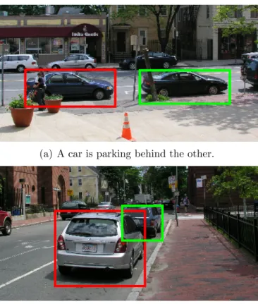
Use of pairwise relations between region/object as spatial context is common [4, 14, 18, 20, 29]. Incorporation of region/object spatial relationships such as above, below, right, left, surrounding, near, etc, into the decision process has been shown to improve the recognition performance in satellite image analysis [1]. However, the models that extract such relationships from a 2D image taken from a top view of the Earth may not be valid for generic views in natural scenes. Since these relationships are not invariant to changes in perspective projection, an actual spatial relationship defined in the real 3D world can be perceived very differently in the image space. Figure 1.2 shows such a setting. In both of the images, the car with the red marker is parked behind the car with the green marker. However, when the 2D spatial relationships of the cars are interpreted, they seem to have different relative positions. Therefore, naming the observed 2D relationships as above, below, etc. does not always make sense in generic views. In [17], we proposed a method that probabilistically infers the real world
CHAPTER 1. INTRODUCTION 6
(a) A car is parking behind the other.
(b) The same relationship from a different angle of view.
Figure 1.2: Similar object relationships in the 3D world can appear in many different configurations in 2D images.
CHAPTER 1. INTRODUCTION 7
Figure 1.3: Overview of the contextual object recognition framework. relationships (defined in 3D space) between objects and use them as spatial con-text. Although the results are promising, the scalability of the context model is problematic due to issues with training real world relationship models.
In this work, we introduce a contextual object recognition framework where the main goal is the determination of the best scene configuration for a still image of a natural indoor/outdoor scene with a complex background and many objects of interest. For this purpose, first, all object detectors are run on the input image. This procedure yields the initial object detections with the class mem-bership probabilities. Then, the contextual interactions among these candidate objects are estimated. Three new spatial relationship features that encode the relative position/location, scale and orientation are extracted for each object pair and used to compute object - object contextual interaction likelihoods. These likelihoods measure the meaningfulness of the interactions (relative position, lo-cation and pose) between the objects. Finally, our framework finds the best scene configuration by maximizing the contextual agreement between the object class labels and their contextual interactions encoded in a novel scene probability function. In our framework, finding the best scene configuration corresponds to
CHAPTER 1. INTRODUCTION 8
the elimination of the objects that are inconsistent with the scene context and the disambiguation of the multiple class labels possible for a single object. The overview of the framework is shown in Figure 1.3.
1.2
Summary of Contributions
Our contextual object recognition framework has three main parts: object de-tection, spatial relationship feature extraction, and contextual agreement maxi-mization. We have contributions for each of these parts. First, we define three methods for object detection. Two of these methods, shape based and pixel classification based object detection, mainly use the techniques presented in the literature. However, we also describe another method called surface orientation based object detection. The goal of that detection technique is to find objects whose shape, color and texture features are not discriminative. Wall, table top, and road are typical examples for such objects. In order to recognize the instances of these object classes, we designed a novel object detector that makes use of the surface orientations. Details are given in Section 2.3.
Another contribution of this work is about spatial relationship features that are the measures of object-object contextual interactions. We define three novel features that encode the relative position, location, scale and orientation ex-tracted from a given object pair. The oriented overlaps feature is the numerical representation of the overlaps observed in the projections of the objects in various orientations. Note that the overlap ratio without orientation is widely used to represent the object relationships. Since an overlap ratio without orientation is a scalar value, it lacks the direction information. On the other hand, our oriented overlaps feature contains rough information regarding the direction based on the orientations. By this way, it can encode the relative position of two objects. The second feature, oriented end points, is designed to represent the relative location of the objects in different orientations. It compares the end points of the objects in the projection space generated by projecting the objects to an orientation of interest. Note that both oriented overlaps and oriented end points are normalized
CHAPTER 1. INTRODUCTION 9
features so that scaling the objects does not change the feature values. Finally, horizontality feature captures the relative horizontality of two objects as a cue about their support relationship. When these features are used in the same prob-abilistic model, inference about the likelihood of the object interactions can be made more robustly. More information about our features and their relation to object interactions are explained in Chapter 3.
The most important contribution is made in the contextual agreement maxi-mization part of our framework. This part combines individual detections (output of the detectors) and the spatial relationships between them to obtain the best scene configuration (best choices for object class labels). For this purpose, we define a novel scene probability function whose maximization results in the con-figuration we seek. This function is defined jointly using individual object class labels and their pairwise spatial relationship features. In addition, it can easily be decomposed into computable probabilistic terms (object detection confidences and object interaction likelihoods). The values of the terms come from object de-tector outputs and the probabilistic contextual interactions models based on our spatial relationship features. Finally, our scene probability function can be easily extended so that its maximization can also lead to additional information about the scene configuration besides object class labels. Such additional information regarding the scene is the type of the relationships (on, under, beside, attached, etc.) between the objects. Complete description of this contextual agreement maximization framework is presented in Chapter 4.
1.3
Organization of the Thesis
The rest of the thesis is organized as follows. In the following chapters, details regarding our contextual object recognition framework are given. Chapter 2 deals with object detector designs we use to obtain initial objects. Next, in Chapter 3, spatial relationship features and object interaction likelihood models are explained. Chapter 4 shows how initial objects and their interactions are used together to reach the best scene configuration. Our data sets and experimental
CHAPTER 1. INTRODUCTION 10
results are presented in Chapter 5. Finally, conclusions together with future work are given in Chapter 6.
Chapter 2
Object Detectors
The first step for building the contextual scene model is the detection of the individual scene elements. In this chapter, important details regarding object detection are discussed.
Object detection is the localization and classification of objects found in the scene. Since each object class carries different characteristics, there is no perfect solution which works for every class. In other words, a universal object detector does not exist. This fact leads to the idea of designing different type of detec-tors for different types of objects. For example, some objects such as cars have distinctive shape properties while their color and texture features demonstrate diversity. Thus, designing a car detector that depends on color features does not make sense. It is better to make a detector that utilizes the shape information to recognize a car. On the other hand, for the grass class, considering shape features is not meaningful. This time, a color based detector may work better because grass tends to appear green. Hence, it is clear that the characteristics of a particular class must be taken into account during detector design.
Although there are differences in the design of detectors, their outputs should be compatible so that they can be handled identically by our framework. This can be achieved by the following requirements. Firstly, the detectors used in our framework must report the object they found as a binary image mask associated
CHAPTER 2. OBJECT DETECTORS 12
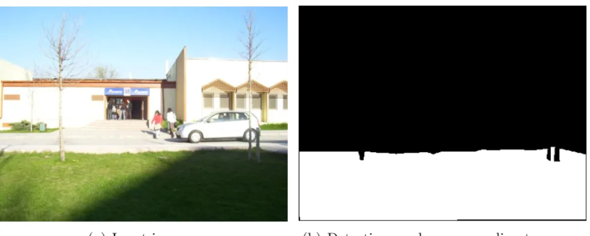
(a) Input image. (b) Detection mask corresponding to grass. Figure 2.1: Sample detection mask.
with a detection confidence score. A sample detection mask is shown in Figure 2.1. Secondly, the confidence scores must be values between 0 and 1, so they can be interpreted as class membership probabilities.
To represent these probabilities, we use the notation P (Xi = c|Di). Here, Xi
is the variable for the object class label and Di is the detector type. Therefore,
P (Xi = c|Di) is the probability of assigning class label c to the i’th object that
is detected by a detector of type Di. Here, detector type, Di, has an
impor-tant role. According to the value of Di, the domain of the object class label
variable, Xi, is determined. Let Di be an object detector that can detect
ob-jects of classes c1, c2, . . . , ck. In this case, the domain of Xi is defined as the set
Ci = {c1, c2, . . . , ck, unknown}. Here, unknown is also crucial because it
corre-sponds to the case of not being able to call an object a member of the set of classes detectable by Di. The unknown label will be used to reject a detection if
it is not compatible with contextual agreement in the scene in Chapter 4. These definitions lead to a final requirement of total probability as
X
u∈Ci
P (Xi = u|Di) = 1. (2.1)
This requirement can be used to compute the probability of Xi being unknown
as
P (Xi = unknown|Di) = 1 −
X
u∈Ci0
CHAPTER 2. OBJECT DETECTORS 13
where Ci0 = Ci− {unknown}.
An example regarding the requirements can be given as follows. Assume that the i’th object is detected by a f lower detector which can recognize the classes rose and tulip. In this case, Di = f lower and Ci = {rose, tulip, unknown}.
This detector must report the following 3 probabilities beside the detection mask corresponding to the i’th object:
1. P (Xi = rose|Di = f lower) = prose,
2. P (Xi = tulip|Di = f lower) = ptulip,
3. P (Xi = unknown|Di = f lower) = 1 − prose− ptulip.
After discussing the detector requirements of our framework, explanations about specific detector designs are given in the rest of this chapter. Although any kind of object detector satisfying the requirements about the mask and the score can be integrated into our framework, we handle three types of detectors in this work. Detectors regarding object classes with discriminative shape prop-erties are described in Section 2.1. Then, in the Section 2.2, pixel classification based approach is presented. Finally, an object detection approach using surface orientations is explained in Section 2.3.
2.1
Shape Based Object Detectors
The details of shape based object detectors are explained in this section. These detectors are useful in finding objects whose color and texture features demon-strate changes across different instances while shape remains nearly unchanged. Objects like car, person and window can be put in this group. In order to deal with such objects, we use two different approaches in our framework:
1. Object detection with boosting [32],
CHAPTER 2. OBJECT DETECTORS 14
The boosting-based detector [32] uses combination of several weak detectors to build a strong detector. Each weak detector performs template matching using normalized cross correlation between the input image and a patch extracted from the training samples. Since patch - object center relationships are available in the training samples, using the correlation output, weak detector votes for the object center. Consequently, weighted combinations of these votes are computed and used to fit bounding boxes on candidate objects. Besides, detection confi-dence scores (class membership probabilities) are reported based on the votes. Original version of this detector works only in a single scale of the image. In order to increase the applicability of the detector, we implemented a multi-scale version using Gaussian pyramids. Note that this is a single class object detector. Thus, a separate detector for each object class is learned using training examples represented using bounding boxes of sample objects.
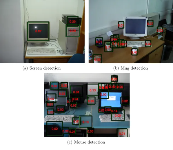
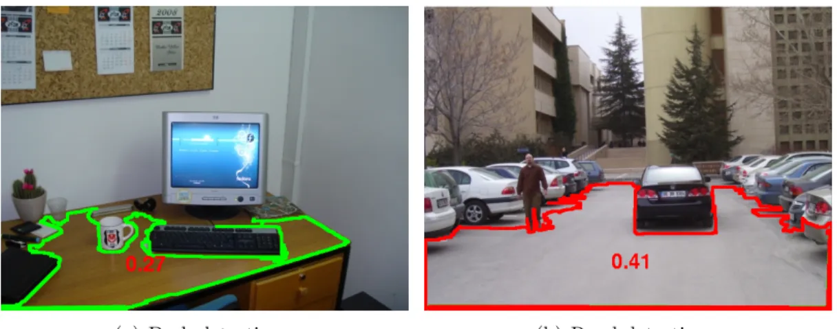
Sample boosting-based detections are shown in Figure 2.2. It is clear that in addition to locating a target object successfully, the detector also reports many false alarms. For objects like mouse that usually looks like a small blob, the num-ber of false alarms can actually be very high. We will show that our framework is good at reducing the false alarm rate by eliminating the detections that are contextually inconsistent. Therefore, we prefer to use these simple detectors that usually do not miss a target object at the expense of several false matches.
The other method we use is HOG based detection [7]. In this method, a sliding window approach is used to detect objects. The image tile under the window is classified and assigned a detection confidence score. During classifica-tion, first of all, HOG features are extracted by dividing the tile into small cells and computing 1D histogram of edge orientations or gradient directions for each cell. To obtain the HOG descriptor of a tile, histograms obtained from the cells are combined. Finally, this descriptor is used in classification of the current tile under the detection window. If a tile is found to be a target object, then it will be reported as a bounding box associated with a confidence score. Note that for better detection outputs, this detector is also run in multiple scales of the input image. Figure 2.3 shows sample detections performed by HOG based detectors.
CHAPTER 2. OBJECT DETECTORS 15
(a) Screen detection (b) Mug detection
(c) Mouse detection
CHAPTER 2. OBJECT DETECTORS 16
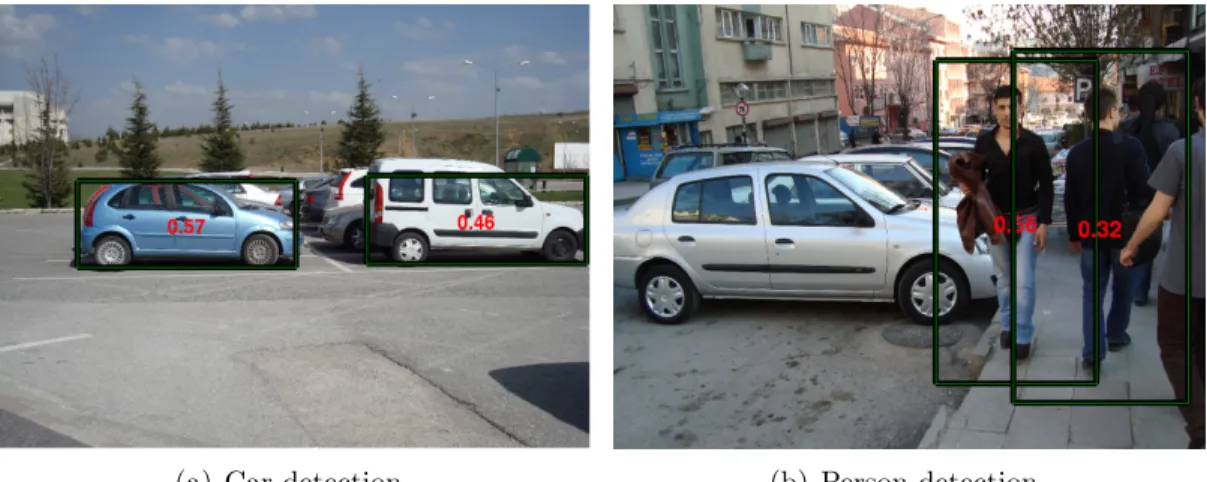
(a) Car detection (b) Person detection Figure 2.3: HOG based detection examples.
In contrast to high false alarm rates of boosting based detectors, HOG based detectors do not tend to report false detections. Although this seems like an advantage, the possibility of missing a target object is higher. Nevertheless, for specific object classes like car and person, we observed that the output of HOG based detectors are more meaningful than the outputs of the boosting based detectors.
Although there are differences in these two shape based detection algorithms, their outputs are identical: bounding boxes and scores. In order to make the detectors compatible with our framework, the bounding boxes are represented as binary image masks.
Another similarity between two approaches is that both detectors work for the single class case. Thus, for the i’th object, the set Ci (possible values of Xi) is
{c, unknown} where c is the particular object class. Then, probabilities reported by the detector should be P (Xi = c|Di = c) and P (Xi = unknown|Di = c).
Using (2.2), P (Xi = unknown|Di = c) is calculated as
P (Xi = unknown|Di = c) = 1 − P (Xi = c|Di = c). (2.3)
For example, consider the leftmost car shown in Figure 2.3(a). In this case, P (Xi = car|Di = car) = 0.57, so P (Xi = unknown|Di = car) must be equal to
CHAPTER 2. OBJECT DETECTORS 17
2.2
Pixel Classification Based Object Detectors
After explaining shape based detection methods, details about pixel classification based approach are given in this section. These detectors are useful in detect-ing objects whose pixel level features (e.g. color, texture) are discriminative for identification. Example classes having this property are grass, soil, sky, etc. In an image, regions corresponding to such objects do not tend to demonstrate a constant shape. Thus, shape based detectors are not good at finding these ob-jects. Instead, in this case, a bottom-up approach where objects are detected by grouping pixels with similar features is used.
At the heart of this method lies pixel classification. So, first of all, a pixel level feature must be defined. For example, sky is made up of blue and white pixels. Thus, choosing RGB as the pixel level feature is intuitive. Secondly, a classifier must be trained based on the chosen feature. This classifier should output a probability of being a pixel of a given object class. In sky detection case, this classifier is expected to report high probabilities when RGB values of a blue or white pixel is given. In order to create such classifiers, in our framework, we use one-class classification using the mixture of Gaussians (MoG) distribution as explained in [30]. It utilizes expectation-maximization algorithm to estimate the mixture weights, means and covariances.
The posterior probability of being a target pixel, P (wT|y), is computed as
P (wT|y) = p(y|wT)P (wT) p(y|wT)P (wT) + p(y|wO)P (wO) = p(y|wT) × 0.5 p(y|wT) × 0.5 + p(y|wO) × 0.5 = p(y|wT) p(y|wT) + p(y|wO) (2.4)
where y is a pixel level feature, wT represents the target class, wO is the case
of being an outlier (non-target) pixel. Then, p(y|wT) is the MoG distribution
learned using examples and p(y|wO) is the uniform distribution assumed for the
outlier pixels. Finally, P (wT) and P (wO) are the prior probabilities for target and
CHAPTER 2. OBJECT DETECTORS 18
be 0.5.
We have explained the training and usage of the pixel level classifiers. Re-call that our main goal is object detection. For this purpose, firstly, features corresponding to each pixel of the given image are extracted. Using these fea-tures and (2.4), each pixel is assigned a probability of being a target object class pixel. Then, pixels with probabilities under a certain threshold are labeled as background. Afterwards, connected components among the remaining forground pixels are extracted. Connected components (regions) with number of pixels less than a threshold are also labeled as background. Then, holes (background pixels) inside each region are filled. These final regions correspond to the image masks, in other words, target object detections. Recall that our framework also requires detection confidence scores. In order to obtain them, posterior probabilities of each pixel of the detected region are averaged and used as confidence scores (class membership probabilities) as P (Xi = c|Di = c) = 1 Mi Mi X j=1 P (c|yj). (2.5)
Here, Mi is the number of pixels in the object (region) and P (c|yj) is the posterior
probability of the j’th pixel of the region. Then, P (Xi = unknown|Di = c) can
be computed as
P (Xi = unknown|Di = c) = 1 − P (Xi = c|Di = c). (2.6)
Although this detector seems to be a single class detector, it can easily be extended to detect multiple classes. Consider the classes grass and tree. When RGB pixel level features of both classes are taken into account, they are not easily distinguishable. In this case, it is better to create a vegetation detector. Let vegetation detector work as a single class pixel classification based object detector. Then, we have the following outputs: P (Xi = vegetation|Di = vegetation),
P (Xi = unknown|Di = vegetation), and the image masks corresponding to
CHAPTER 2. OBJECT DETECTORS 19
(a) Sky detection. (b) Vegetation detection. Figure 2.4: Pixel classification based object detection examples. can be computed as
P (Xi = grass|Di) = P (Xi = vegetation, Xi = grass|Di)
= P (Xi = grass|Xi = vegetation, Di)P (Xi = vegetation|Di)
= P (Xi = grass|Xi = vegetation)P (Xi = vegetation|Di).
(2.7) Note that every grass is also a vegetation object. Thus, event of {Xi = grass} is
identical to the event of {Xi = vegetation ∩ Xi = grass}.
Similarly, P (Xi = tree|Di = vegetation) is calculated as
P (Xi = tree|Di) = P (Xi = tree|Xi = vegetation)P (Xi = vegetation|Di).
(2.8) Probabilities, P (Xi = grass|Xi = vegetation) and P (Xi = tree|Xi =
vegetation), are estimated using a training set with manual object labels as P (Xi = grass|Xi = vegetation) =
#(vegetation objects labeled as grass) #(vegetation objects)
(2.9) and
P (Xi = tree|Xi = vegetation) =
#(vegetation objects labeled as tree)
#(vegetation objects) , (2.10) respectively.
CHAPTER 2. OBJECT DETECTORS 20
In multiclass version, computation of P (Xi = unknown|Di = c) is still
per-formed using (2.6).
Sample pixel based object detection outputs are shown in Figure 2.4.
2.3
Surface Orientation Based Object Detectors
We have discussed the cases where objects have discriminative features like spe-cific shape, color and texture. However, there are also object classes which do not demonstrate a pattern in terms of these features. Instances of such classes usu-ally appear in arbitrary but uniform color and texture. For example, wall, table top, floor and ceiling share this property. Consider a circular wooden table and a rectangular plastic table. They seem completely different, so classifying them into same class using specific values of their color, texture or shape features does not make sense. Objects demonstrating this property are called surface objects in our framework.
Hoiem [16] developed a method for recovering the surface layout from a single still image. The method labels the regions of an image with geometric classes like support and vertical. Support regions refer to the objects that are approximately parallel to the ground (eg. road, table tops). Vertical image areas correspond to the objects such as walls, trees, pedestrians and buildings. We use this method to obtain confidence maps for the geometric classes horizontal (0 degree) and vertical (90 degrees) relative to the ground plane.
Detection of surface objects begins with finding associated image regions. In order to do so, we group the individual pixels into few partitions by applying k-means clustering to the verticality and horizontality confidences of pixels. For k-means clustering, each pixel’s horizontality and verticality confidence are con-catenated and used as feature vector. After clustering, connected components are extracted using pixels assigned to same group. Components with number of pixels less than a threshold are labeled as background. Remaining ones are kept as image masks showing detected surface objects.
CHAPTER 2. OBJECT DETECTORS 21
Second step in the detection is the determination of class membership prob-abilities of the detected objects. For this purpose, again we use the verticality and horizontality confidence maps. First of all, the horizontality and vertical-ity probabilities for each detected surface object are computed by averaging the values in the corresponding regions of the confidence maps. We denote the hor-izontality and verticality probabilities as P (Gi = horizontal |Di = surface) and
P (Gi = vertical |Di = surface), respectively, where Gi represents the geometric
class label and Di represents the type of the detector. The probability of a surface
not being horizontal or vertical is computed as
P (Gi = unknown|Di = surface) = 1 − P (Gi = horizontal |Di = surface)
− P (Gi = vertical |Di = surface).
(2.11)
The horizontal and vertical surfaces can be further divided into categories such as road, table, etc. for horizontal, and wall, building, etc. for vertical. The i’th object’s probability of being a surface object of type c can be computed as
P (Xi = c|Di = surface) = X Gi P (Xi = c, Gi|Di = surface) =X Gi P (Xi = c|Gi)P (Gi|Di = surface). (2.12)
Note that P (Xi = c|Gi = horizontal ) = 0 if c is not a horizontal surface type,
P (Xi = c|Gi = vertical ) = 0 if c is not a vertical surface type, and P (Xi =
unknown|Gi = unknown) is always equal to 1. Then probabilities for horizontal
objects are computed as P (Xi = ch|Di = surface)
= P (Xi = ch|Gi = horizontal )
P (Gi = horizontal |Di = surface) (2.13)
and the probabilities for vertical objects are computed as P (Xi = cv|Di = surface)
= P (Xi = cv|Gi = vertical )
CHAPTER 2. OBJECT DETECTORS 22
(a) Desk detection. (b) Road detection. Figure 2.5: Surface orientation based detection examples.
where P (Xi = ch|Gi = horizontal ) and P (Xi = cv|Gi = vertical ) are estimated
from the percentage of the number of horizontal surface objects labeled as ch
among all horizontal surface objects, and the percentage of the number of verti-cal surface objects labeled as cv among all vertical surface objects, respectively.
Finally, the possibility of not being able to label a surface object is modeled by the probability
P (Xi = unknown|Di = surface)
=X
Gi
P (Xi = unknown|Gi)P (Gi|Di = surface)
= P (Xi = unknown|Gi = unknown)P (Gi = unknown|Di = surface)
= P (Gi = unknown|Di = surface).
(2.15)
Chapter 3
Interactions Between Scene
Components
Contextual interactions observed in a scene must be incorporated into the de-cision process about that scene to achieve a better detection performance. A candidate interaction is the co-occurrence of the objects. Learning this contex-tual information is relatively easy when the data set contains an adequate number of groundtruth class label assignments. However, co-occurrences alone may not be sufficient to encode the whole context in the scene. For example, cars and buildings tend to co-occur, but it is not usual to observe a building located under a car. Suppose these objects are accidentally detected in the scene. Since they are consistent according to the co-occurrence likelihood, the system will favor such unreasonable configuration.
Therefore, a more sophisticated system should consider the relative posi-tions/locations, scales and orientations observed among the objects. This cor-responds to the use of spatial realtionships. If a system is aware of the most likely spatial relationships between the objects, it can handle unlikely situations with a higher precision. Algorithms that can model topological (set relationships, adjacency), distance-based (near, far) and relative position-based (above, below,
CHAPTER 3. INTERACTIONS BETWEEN SCENE COMPONENTS 24
right, left) relationships have been successfully applied to satellite image analy-sis for improving the classification accuracy [1]. However, relationships that are defined in the 2D image space are not always applicable to generic scene analysis because object relationships in the 3D world can appear in many different con-figurations in a 2D image. Example images for these concon-figurations are shown in Figure 1.2. In these images, the car with the red marker is parked behind the car with the green marker. However, when the 2D spatial relationships of the cars are interpreted, they seem to have different relative positions. Hence, naming the spatial relationships by just analyzing the relative positions is problematic.
Although both ways of handling context have some disadvantages, they can be combined into a more powerful approach. In our proposed method, co-occurence likelihood’s robustness to the wrong estimations of the spatial relationship types and the strength of relative position/location, scale and orientation are handled in the same probabilistic model. For this purpose, three different spatial relationship features are introduced and explained in Section 3.1. Then, we mention how we use these features to estimate object interaction likelihoods in Section 3.2.1. Since we have chosen co-occurrence likelihoods as a baseline approach to be compared with our proposed model during experiments (Chapter 5), we also explain how co-occurrence probabilities can be utilized as interaction likelihoods in Section 3.2.2.
3.1
Spatial Relationship Features
A single spatial relationship feature is not sufficient to describe the observed relationship between objects. Therefore, we use multiple features to encode the interactions. By this way, we can analyze the pairwise interactions from different perspectives and take advantage of different measures.
Feature values are calculated using the binary image masks corresponding to the objects. Since features used in our framework are relative, during feature extraction for an object pair, one of them is chosen as the reference object.
CHAPTER 3. INTERACTIONS BETWEEN SCENE COMPONENTS 25
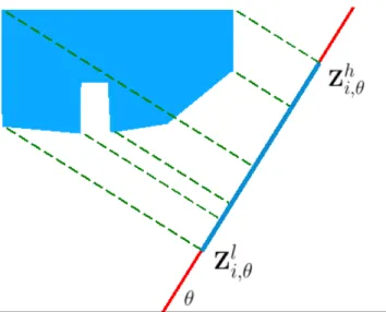
Figure 3.1: Projection of an object onto the line with orientation θ. Blue region: object to be projected, red line: orientation of projection, blue line segment: projected object.
Throughout this section, suppose that spatial relationship features are extracted for object oi with respect to reference object oref.
Let Pi be the set of pixels constituting the object oi and Zi be the 2 × Mi
matrix whose columns are the (x, y)-coordinates of oi’s pixels (foreground pixels
in the binary image mask) where Mi = |Pi|. Then,
Zi =
"
xi,1 xi,2 xi,3 . . . xi,Mi
yi,1 yi,2 yi,3 . . . yi,Mi
#
. (3.1)
Some of the features we will introduce require projections of the objects. Let Aθ be the transformation matrix which projects the objects onto the line with
orientation θ relative to the horizontal axis as Aθ =
h
cos θ sin θ i
. (3.2)
Then, Zi,θ is the 1 × Mi vector containing pixel coordinates in the projected space
as
CHAPTER 3. INTERACTIONS BETWEEN SCENE COMPONENTS 26
An example projection is given in Figure 3.1. When an object is projected on a line, the image region corresponding to that object is converted to a line segment. For some features, end points of this line segment are required. Lower and higher end points are denoted by Zl
i,θ and Zhi,θ, respectively as
Zli,θ = min {Zi,θ} (3.4)
Zhi,θ = max {Zi,θ}. (3.5)
Details of our spatial relationship features are explained in the following sub-sections.
3.1.1
Oriented Overlaps Feature
Overlap ratios of two regions are widely used features. An example of its usage can be seen in [13]. It is simply calculated by dividing the number of pixels in the overlapping area by the number of pixels in one of the objects. However, this simple feature does not capture the relative location of the participating regions. Thus, it is not sufficient to encode the observed relationship. To overcome this issue, overlap features are mostly used with relative centroid positions. Since centroid of an object with arbitrary shape is not always representative enough to describe the location of the entire object, this combined feature does not work as expected. In addition, the units of overlap ratio and centroid differences are not compatible (while overlap ratio is unitless, centroid feature is measured in pixels). Therefore, the feature space generated by the combination of these features is not meaningful.
Here, we introduce an overlap based feature called oriented overlaps. It en-codes the relative overlap and position in a unified representation. This feature is extracted as follows. First of all, some orientations of interest are selected. Let the set of these orientations be Θ = {θ1, θ2, . . . , θ|Θ|}. Then, for each element
of Θ, Zlref,θj and Zhref,θj are computed, where 1 < j < |Θ|. Recall that these represent the lower and higher end points of the line segment corresponding to the object oref in the projection space, respectively. Let the set Pi,ref,θj be the
CHAPTER 3. INTERACTIONS BETWEEN SCENE COMPONENTS 27
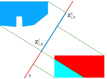
Figure 3.2: The computation of ρi,ref,θj. Here, the reference object, oref, is shown
as a blue region. The object whose oriented overlaps feature is being computed, oi, is shown as a red-cyan region. The red portion of oi is composed of the
pixels whose projections are values in the [Zlref,θj, Zhref,θj] interval (the blue line segment). Thus, ρi,ref,θj is calculated as (number of oi’s red pixels)/(total number
of oi’s pixels).
subset of oi’s pixels whose projections are values in the [Zlref,θj, Z
h
ref,θj] interval.
Then, the overlap ratio, ρi,ref,θj, observed in orientation θj is calculated as
ρi,ref,θj =
|Pi,ref,θj|
Mi
. (3.6)
Illustration corresponding to the computation of ρi,ref,θj is shown in Figure
3.2.
The oriented overlaps feature vector, Oi,ref, is formed by concatenating the
features for all orientations as Oi,ref =
h
ρi,ref,θ1 ρi,ref,θ2 ρi,ref,θ3 . . . ρi,ref,θ|Θ|
i
. (3.7)
In our framework, to keep the feature space simple enough, we chose Θ as the set {0, 90}. Although information coming from other orientations is also important, in order to avoid high dimensionality problems, we preferred 0 and 90 degree orientations.
CHAPTER 3. INTERACTIONS BETWEEN SCENE COMPONENTS 28
Figure 3.3: Oriented overlaps feature space. While x-axis shows values of ρi,ref,0,
y-axis corresponds to ρi,ref,90. Features are extracted for the red object (oi) with
CHAPTER 3. INTERACTIONS BETWEEN SCENE COMPONENTS 29
are the features extracted using object pairs found in one of the data sets (a subset of LabelMe [27]) we use in the experiments. The double-headed arrows show how the relationship between the red (oi) and green (oref) boxes change as
the feature values vary in the specified direction. Note that the range of feature values is [0, 1] for both ρi,ref,0 and ρi,ref,90.
Consider the boxes shown in group A. Using any of the four red boxes in feature extraction with the green box (the reference object) results in the same feature vector, (0, 0). As ρi,ref,0 (x-axis) increases, the positions of the red boxes
change as shown in the transitions A → H, H → G, C → D and D → E. Similarly, as ρi,ref,90 (y-axis) value increases, the positions change as shown in
the transitions A → B, B → C, G → F and F → E.
Note that although there are usually more than one possible relative position for a single oriented overlaps feature vector, the relationship observed in each position is similar regardless of the direction.
3.1.2
Oriented End Points Feature
Although the oriented overlaps feature is informative about the relative positions, it cannot distinguish the spatial relationships in which direction is important. For example, a mouse can be found either on the left or right of a keyboard. It is clear that direction of the relationship is not significant in the keyboard and mouse case, so the oriented overlaps feature is sufficient to encode the relationship between them. However, the situation is different for the grass and sky classes. In a natural scene, the sky is expected to appear above the grass. But, if the oriented overlaps feature is used, observing sky below the grass will be encoded similarly. The reason is that the oriented overlaps feature encodes only the amount of overlap (a scalar value, i.e. no direction information) in different orientations.
In order to distinguish the relationships in which direction is also important besides the orientation, we define another feature called oriented end points. Ex-traction of this feature is as follows. First of all, an orientation of interest, θ,
CHAPTER 3. INTERACTIONS BETWEEN SCENE COMPONENTS 30
Figure 3.4: An example computation of Ei,ref,θ. Here, the reference object, oref,
is shown as a blue region. The object whose oriented end points feature is being computed, oi, is shown as a green region. After the projection and normalization
steps, the end points of the objects take the values shown in the figure. Thus, Ei,ref,θ is computed as (−1.69, 0.28).
is selected. Then values, Zl
i,θ, Zhi,θ, Zlref,θ and Zhref,θ, are calculated. Recall that
these values are the end points of the line segments representing the objects in the space of projection.
This feature is expected to encode the relative positions of the line segments. For this purpose, a transformation function, Γ, that normalizes the reference object’s line segment is defined as
Γ(z) = 2z − Z l ref,θ − Zhref,θ Zh ref,θ − Zlref,θ (3.8)
where Γ(Zlref,θ) = −1.00 and Γ(Zhref,θ) = 1.00. Using the same transformation function, oriented end points feature, Ei,ref,θ, is constructed as
Ei,ref,θ = h Γ(Zl i,θ) Γ(Zhi,θ) i . (3.9)
Since this is a normalized feature, it encodes both the relative position and the relative scale in the same representation.
CHAPTER 3. INTERACTIONS BETWEEN SCENE COMPONENTS 31
Figure 3.5: Oriented end points feature space for θ = 0. While x-axis shows values of Γ(Zli,0), y-axis corresponds to Γ(Zhi,0). Features are extracted for the red object (oi) with respect to the green object (oref). See text for more details.
CHAPTER 3. INTERACTIONS BETWEEN SCENE COMPONENTS 32
Figure 3.6: Oriented end points feature space for θ = 90. While x-axis shows values of Γ(Zl
i,90), y-axis corresponds to Γ(Zhi,90). Features are extracted for the
CHAPTER 3. INTERACTIONS BETWEEN SCENE COMPONENTS 33
In our framework, we extract oriented end points features for orientations 0 and 90. Therefore, there are two feature vectors, Ei,ref,0 and Ei,ref,90, to be
extracted for each object pair.
Figure 3.5 shows the feature space for oriented end points feature where θ = 0. Blue dots are the features extracted using object pairs found in the subset of LabelMe images. The double-headed arrows show how the relationship between the red (oi) and green (oref) boxes change as the feature values vary in the
specified direction. Note that Γ(Zl
i,0) ≤ Γ(Zhi,0) and the range of feature values is
(−∞, +∞) for both Γ(Zl
i,0) and Γ(Zhi,0).
As the Γ(Zl
i,0) (x-axis) increases, the size of the red object decreases as shown
in transitions C → D and D → E. On the other hand, when Γ(Zh
i,0) (y-axis)
increases, the size of the object increases as shown in transitions A → B and B → C. Note that besides changes in size, the position of the red object also varies in those transitions. The diagonal transitions like A → F and F → E affect only the position of the red object. On the contrary, the transition F → C changes the size instead of the position.
The feature space of oriented end points where θ = 90 is available in Figure 3.6. This figure can be similarly interpreted as the feature space shown in Figure 3.5.
3.1.3
Horizontality Feature
We have explained two spatial relationship features that try to encode relative position and scale observed between objects. Both features are extracted using the observations from the 2D image space. However, objects are found in a 3D environment in real world. Therefore, in order to encode a relationship, infor-mation coming from 3D space is also useful. The horizontality feature is defined for this purpose. This feature measures the relative horizontality confidence of oi
with respect to oref. Recall the Hoiem’s technique [16] to find surface layout from
CHAPTER 3. INTERACTIONS BETWEEN SCENE COMPONENTS 34
Section 2.3. In order to extract the horizontality feature, the horizontality confi-dence for oi and oref are computed by averaging the values in the corresponding
regions of the horizontality confidence map. Let Hi and Href be the confidence
values of the objects. The scalar horizontality feature, Hi,ref, is simply calculated
as
Hi,ref = Hi− Href. (3.10)
There is no need to compute a verticality feature, because there is a high correlation between horizontality and verticality. In [16], for each image, confi-dence maps for three main classes are extracted: support, vertical, and sky, where the sum of three confidence values for a pixel is equal to 1. Therefore, relative verticality is equal to
Vi− Vref = (1 − Hi− Skyi) − (1 − Href − Skyref)
= −(Hi− Href) − (Skyi− Skyref)
= −Hi,ref − (Skyi− Skyref).
(3.11)
For objects other than sky, (Skyi− Skyref) ' 0, so relative verticality is
approx-imately equal to −Hi,ref. Therefore, using horizontality feature is sufficient.
Feature space for Hi,ref is simple. It takes values from −1 to 1 inclusively. As
the value approaches to −1, verticality of oi increases. Conversely, values close
to 1 shows that object is more horizontal. For example, Hscreen,desk is expected
to have a value closer to −1.
3.2
Object Interaction Likelihood
The meaningfulness of the interactions (co-occurrence, relative position, loca-tion and pose) between objects can be measured in terms of interacloca-tion likeli-hoods that are computed with respect to the training examples. It is denoted as p(Si,j|Xi, Xj). This is the probability of observing Si,j, the interaction between
CHAPTER 3. INTERACTIONS BETWEEN SCENE COMPONENTS 35
We focus on how the spatial relationship features and the co-occurrence prob-abilities are utilized to represent the object interactions in Sections 3.2.1 and 3.2.2, respectively.
3.2.1
Spatial
Relationship
Feature
Based
Interaction
Likelihood
In our proposed method, we use the spatial relationship features to estimate how likely a particular interaction between two objects is by learning probabilistic models for each object class pair using these features. Then, for a new object pair, likelihood of the interaction is computed using the associated model. The value of p(Si,j|Xi, Xj) is calculated as
p(Si,j|Xi, Xj) =
Y
ωi,j∈Ωi,j
p(ωi,j|Xi, Xj) (3.12)
where Ωi,j is the set of spatial relationship features extracted for the (oi, oj) pair.
In the full probabilistic model, Ωi,j is taken as the set {Oi,j, Ei,j,0, Ei,j,90, Hi,j}.
Then, p(Si,j|Xi, Xj) is computed as
p(Si,j|Xi, Xj) = p(Oi,j|Xi, Xj)p(Ei,j,0|Xi, Xj)p(Ei,j,90|Xi, Xj)p(Hi,j|Xi, Xj).
(3.13) Note that using full model is not mandatory. Any subset of the full set can be used to estimate interaction likelihoods.
Individual p(ωi,j|Xi, Xj)’s are calculated as smoothed histogram estimates.
For this purpose, from a training set where individual objects are manually la-beled, we collect feature vectors for each object class pair like (screen, desk ), (sky, building), (keyboard, keyboard ), (grass, road ), etc. Since our feature vectors are extracted with respect to a reference object, we also collect features for (desk, screen), (building, sky) and (road, grass) pairs. This means that we extract two feature vectors for each object class pair due to possible asymmetry in the cor-responding relations. Then, we estimate the object pair conditional density of
CHAPTER 3. INTERACTIONS BETWEEN SCENE COMPONENTS 36
Table 3.1: Properties of the spatial relationship feature histograms.
Feature #Bins Range Gaussian Kernel
Oriented overlaps 20 × 20 ρi,ref,0 ∈ [0, 1] 3 × 3
ρi,ref,90∈ [0, 1] σ = 0.75
Oriented end points 20 × 20 Γ(Zl
i,0) ∈ [−50, 50] 3 × 3
(θ = 0) Γ(Zh
i,0) ∈ [−50, 50] σ = 0.75
Oriented end points 20 × 20 Γ(Zl
i,90) ∈ [−50, 50] 3 × 3
(θ = 90) Γ(Zhi,90) ∈ [−50, 50] σ = 0.75
Horizontality 1 × 20 Hi,ref ∈ [−1, 1] 1 × 3
σ = 0.75
these features, pω
u,v(ωi,j), using the non-parametric histogram estimate as
pωu,v(ωi,j) = kω u,v(ωi,j) nω u,vVu,vω (3.14) where kωu,v(ωi,j) is the value in the histogram bin where ωi,j falls in, nωu,v is the
sum of the values in all bins and Vω
u,v is the bin volume. Note that the histogram
estimates of (building, sky) and (sky, building) pairs are not the same. The original histograms may not be appropriate for the estimation of pω
u,v(ωi,j)
values due to zero frequency problem and sharp changes in the adjacent bins. Thus, we assume a uniform prior by incrementing each histogram bin by one in order to avoid zero frequency problem observed due to zero counts in the his-tograms. Moreover, we avoid sharp changes in the adjacent bins by smoothing the histogram using a Gaussian kernel. Consequently, we obtain the final smoothed histograms that are used to calculate the interaction likelihood for a new object pair. Table 3.1 summarizes the properties of the histograms for oriented overlaps, oriented end points and horizontality features. Note that although the range of oriented end points feature values is (−∞, +∞), we limit the range of these val-ues to [−50, 50] in the histograms. The reason is that feature vectors out of this range are not observed very frequently and the number of bins does not need to be significantly increased for such rare cases. Thus, any value less than −50 is mapped to −50 and any value greater than 50 is replaced by 50.
![Figure 1.1: Example of object (coffee machine) - scene (kitchen) interaction [33].](https://thumb-eu.123doks.com/thumbv2/9libnet/5915907.122673/19.918.306.786.174.473/figure-example-object-coffee-machine-scene-kitchen-interaction.webp)