2012 IEEE INTERNATIONAL WORKSHOP ON MACHINE LEARNING FOR SIGNAL PROCESSING, SEPT. 23–26, 2012, SANTANDER, SPAIN
EXTRACTION OF SPARSE SPATIAL FILTERS USING OSCILLATING SEARCH
Ibrahim Onaran
1,2, N. Firat Ince
1,3, Aviva Abosch
1, A. Enis Cetin
21
Department of Neurosurgery, University of Minnesota, Minneapolis, MN 55455 USA
2Department of Electrical Engineering, Bilkent University, Ankara, Turkey
3
Department of Electrical and Computer Engineering,
University of Minnesota, Minneapolis, MN 55455 USA
ABSTRACT
Common Spatial Pattern algorithm (CSP) is widely used in Brain Machine Interface (BMI) technology to extract features from dense electrode recordings by using their weighted lin-ear combination. However, the CSP algorithm, is sensitive to variations in channel placement and can easily overfit to the data when the number of training trials is insufficient. Construction of sparse spatial projections where a small sub-set of channels is used in feature extraction, can increase the stability and generalization capability of the CSP method. The existingℓ0 norm based sub-optimal greedy channel re-duction methods are either too complex such as Backward Elimination (BE) which provided best classification accura-cies or have lower accuracy rates such as Recursive Weight Elimination (RWE) and Forward Selection (FS) with reduced complexity. In this paper, we apply the Oscillating Search (OS) method which fuses all these greedy search techniques to sparsify the CSP filters. We applied this new technique on EEG dataset IVa of BCI competition III. Our results indicate that the OS method provides the lowest classification error rates with low cardinality levels where the complexity of the OS is around 20 times lower than the BE.
Index Terms— Brain Machine Interface,
Electroen-cephalogram (EEG), Sparse Filter, Oscillating Search
1. INTRODUCTION
BMI research seeks to develop technologies that enable pa-tients to communicate with their environment solely through the use of brain signals. Recent advances in electrode design and recording technology allow for recording of neural data from large numbers of electrodes. These large electrode ar-rays are used to sample a greater brain region, or to obtain more detailed information from a smaller portion of the brain using a dense setup. The increased number of recording chan-nels demands greater computational power and has the po-tential to introduce irrelevant or highly-correlated channels. The CSP algorithm is a widely used method to decrease the computational complexity of the classification algorithms as
well as to decrease the correlation between channels and im-prove the signal-to-noise ratio (SNR) of multichannel record-ings from both noninvasive and invasive modalities [1, 2].
The CSP method is a useful tool to solve the problems re-lated to the number of channels by linearly combining chan-nels into a few virtual chanchan-nels. The CSP method forms new virtual channels by maximizing the Rayleigh Quotient (RQ) of the spatial covariance matrices. This procedure creates a variance imbalance between the classes of interest. The RQ is defined as
𝑅(𝑤) = 𝑤𝑤𝑇𝑇𝐵𝑤𝐴𝑤 (1) where𝐴 and 𝐵 are the spatial covariance matrices of two dif-ferent classes and𝑤 is the spatial filter or the virtual channel. Although useful, the CSP method has also some disadvan-tages. The most common problem of the CSP method is that it generally overfits the data when the number of trials is limited and when the signal is recorded from a large number of chan-nels. Moreover, the chance of recording corrupted or noisy signal is increased with the number of recording channels. Since all channels are used in spatial projections of CSP, the classification accuracy may be reduced in situations in which electrode location varies slightly between different recording sessions. This requires nearly identical electrode spatial loca-tion over time, which is difficult to realize [3].
To address the drawbacks of the traditional CSP method, various sparse spatial filter methods are used by researchers [4–8]. These methods attempted to compute sparse CSP (sCSP) filters by converting CSP into a quadratically con-strained quadratic optimization problem withℓ1 penalty [5] or used anℓ1/ℓ2 norm based regularization parameter with the traditional CSP method [4, 6]. The authors of [4, 5] have reported a slight decrease or no change in the classification accuracy while decreasing the number of channels signif-icantly. Recently, in [7] a quasi ℓ0 norm based criterion was used for obtaining the sparse solution, which resulted in an improved classification accuracy. Since ℓ0 norm is non-convex, combinatorial and NP-hard, they implemented greedy solutions such as forward selection (FS) and backward elimination (BE) to decrease the computational complexity. 978-1-4673-1026-0/12/$31.00 c⃝2012 IEEE
It was shown that the less myopic BE method out-performs the FS method with a dramatically higher computational cost. In [8] recursive weight elimination is proposed which has lower complexity and comparable classification accuracy with BE with higher cardinality, which is the number of non-zero entries in the sparse spatial filter. In [9] CSP patches (CSPP) is employed to fuse Laplacian filters and the CSP method. In this method, the CSP filters are calculated on
predefined channel groups. The results obtained from CSPP
filters are compared to the results obtained from Laplacian, traditional CSP and regularized CSP filters. They report that CSPP method outperforms other methods in case of only a very few calibration data is available. The main disadvan-tage of this method is that we need to know the predefined channels before applying CSP method. In [10], Support Vector Channel Selection (SVCS) adapts the Recursive Fea-ture Elimination (RFE) and Support Vector Machine (SVM) classifier for the purpose of selecting EEG channels. They extract features from each channel and eliminate a channel that has features resulting minimum score at each step. They showed that the number of channels can be reduced signifi-cantly without increasing classification error and the resulting channels agree with the underlying cortical activity patterns of the mental task. Unlike SVCS, OS eliminates the channels on sample space according to the coherent activity of the channels. Therefore, OS is significantly different from the method described in [10].
In this paper, we fuse all the greedy techniques to obtain sparse filters yielding low classification error rates with re-duced computational complexity. In this scheme, we used the oscillating search, a subset selection technique from a large set of features [11, 12]. Unlike the BE, FS or RWE, the OS does not operate in a fixed direction. We show that using the OS method one can extract sparse filters at low cardinalities with lower complexity and error rates. The rest of the paper is organized as follows. In the following section, we describe the greedy search algorithms and their relations with the new OS algorithm. Next, we apply our method on the BCI com-petition III EEG dataset IVa [13, 14] involving imaginary foot and hand movements. We also compare our method to stan-dard CSP and other greedy search algorithms such as BE, FS and RWE. Finally, we discuss our results and provide future directions.
2. MATERIAL AND METHODS 2.1. Standard CSP Method
In the CSP framework, the spatial filters are a weighted linear combination of recording channels, which are tuned to pro-duce spatial projections maximizing the variance of one class and minimizing the other. The spatial projection is computed using
𝑋𝐶𝑆𝑃 = 𝑊𝑇𝑋 (2) where the columns of𝑊 are the vectors representing each spatial projection and𝑋 is the multichannel ECoG data.
Since RQ (1) does not depend on the magnitude of 𝑤, maximizing the RQ is identical to the following optimization problem. maximize 𝑤 𝑤 𝑇𝐴𝑤 subject to 𝑤𝑇𝐵𝑤 = 1. (3) After writing this optimization problem in the Lagrange form and taking the derivative with respect to𝑤, we obtain the identical problem in the form of𝐴𝑤 = 𝜇𝐵𝑤 which is the Generalized Eigenvalue Decomposition (GED). The solutions of this equation are the joint eigenvectors of𝐴 and 𝐵 and 𝜇 is the associated eigenvalue of a particular eigenvector.
2.2. Sparse CSP Methods
The drawbacks of the CSP method that are described earlier prompted us to find a way to sparsify the spatial filter to in-crease the classification accuracy and the generalization ca-pability of the method. We assumed that the discriminatory information is embedded in a few channels where the ber of these channels is much smaller than the actual num-ber of all recording channels. So the discrimination can be obtained with a sparse spatial projection, which uses only in-formative channels. In this scheme assume that the data was recorded from𝐾 channels. The spatial projections 𝑤 has only
𝑘 nonzero entries, 𝑐𝑎𝑟𝑑(𝑤) = 𝑘 and 𝑘 ≪ 𝐾. We are
inter-ested in obtaining a sparse spatial projection using OS, BE, RWE and FS.
The FS and BE are described in detail in [15]. It is known that finding a sparse solution usingℓ0norm is combinatorial and NP-hard. Therefore they suggested greedy search meth-ods to sparsify the CSP filter. The methmeth-ods are described be-low.
The covariance matrices𝐴 and 𝐵 can be computed using the training data and assuming the sparse solution𝑤 where most of the entries in𝑤 are zero, is given. That means 𝑤 satisfy the following optimization equation.
arg max 𝑤
𝑤𝑇𝐴𝑤
𝑤𝑇𝐵𝑤 s.t.∥𝑤∥0= 𝑘. (4) It is observed that the sparse vector𝑤 selects the column and rows of the matrices𝐴 and 𝐵, so the Equation 4 can be rewritten as, arg max 𝑤𝑘 𝑤𝑇 𝑘𝐴𝑘𝑤𝑘 𝑤𝑇 𝑘𝐵𝑘𝑤𝑘 s.t.∥𝑤𝑘∥0= 𝑘. (5)
where𝐴𝑘and𝐵𝑘are the matrices that have only the rows and columns those correspond to the nonzero entries of the sparse
solution𝑤 and 𝑤𝑘has only nonzero entries of the sparse so-lution𝑤. That means the reduced matrices 𝐴𝑘and𝐵𝑘are the
𝑘 × 𝑘 submatrices of the original covariance matrices. The
problem here is which sub-matrix should be selected. Search-ing all possible submatrices is infeasible and involvesℓ0norm optimization problem. FS or BE can be used to obtain subop-timal solutions of this original problem.
2.2.1. Forward Search
The FS starts with an empty set of channels. It solves the CSP problem for all individual channels that are not in the current channel set and adds the channel that has resulted maximum variance increase to the current set. The procedure continues with other cardinality levels sequentially until the required cardinality level is reached. FS solves𝐾 − 𝐶 CSP problems for(𝐶 + 1) × (𝐶 + 1) matrices where 𝐾 is the total number of channels and𝐶 is the number of elements in the current set. In each step we increase number of channels by adding a channel to the current set until we reach the desired cardinal-ity𝑘. So the computational complexity would be increased with the desired cardinality𝑘. This algorithm depends on 𝐾 linearly for a particular𝑘, so increasing the number of chan-nels does not affect the complexity of the algorithm as much as BE. However the results indicate that the accuracy of this method is less than the BE.
2.2.2. Backward Elimination
The BE starts with all channels and it removes the channels in the set one by one and solves the CSP for each channel in the set. The channel that has resulted maximum variance de-crease is eliminated. The procedure continues for the remain-ing channels in the set until we reach the desired cardinality. The BE method in the first step searches𝐾 − 1 separate sub-matrices and solves GED problem for each of them to find a sparse solution whose cardinality is𝐾 − 1. Hence, a GED is solved𝐾 − 1 times on 𝐾 − 1 × 𝐾 − 1 matrices. In each step the size of the submatrices become one less and that is also equal to the number of separate GED solutions that is performed at each step. As a result, until the desired cardi-nality is reached the total number of separate GED solutions dominates the computational complexity. The computational complexity is even higher when𝐾 is large and the desired cardinality is small. Since the number of CSP computations and the size of the matrices those involve in CSP solution both depend on𝐾, the effect of 𝐾 is much apparent when 𝐾 is increased for BE method.
2.2.3. Recursive Weight Elimination
The RWE approach is recently introduced by [8], motivated by the work of [16] which employed a recursive feature elim-ination in an SVM framework.
The RWE starts with all channels and it removes the chan-nels in the set one by one and solves the GED problem for each channel in the set. The difference between the RWE and the BE is the elimination strategy. The BE solves the GED for each submatrix by removing a channel at a time from the fullset and eliminates the channel which provided the mini-mum drop in RQ. On the other hand RWE solves GED using all channels in the current set and finds the entry in the spatial filter that has the minimum absolute amplitude. The corre-sponding channel is removed from the set. The procedure continues for the remaining channels in the set until we reach the desired cardinality. Therefore, a GED is solved only once on𝐶 × 𝐶 matrix in each step where 𝐶 is the current car-dinality level of sparse matrix 𝑤 in the current step. As a result, the computational complexity of RWE is dramatically low and decreases in each step.
2.2.4. Oscillating Search
The oscillating search (OS) approach is motivated by the work of [11, 12]. They used OS method to select a subset of features from a large set in a computationally efficient manner. In this scheme the OS uses an upswing and a down swing procedure, by running forward addition and backward elimination, steps to modify an initial (given) set of features based on a cost criterion. The initial set is either selected randomly or using a method that requires low computational power.
Here, with the same spirit, we used OS to extract a sparse spatial filter solutions by fusing FS, BE and RWE methods. Assume that we are searching for a sparse filter with cardinal-ity𝑘. In order to select the initial set, we used RWE method, which is dramatically faster than BE and more accurate than FS with comparable computational complexity. After obtain-ing the initial set of𝑘 channels, we executed the up and down swing steps to modify it. We used the RQ as a criterion to assess the effectiveness of each identified subset. During the upswing procedure, simply, we added channels using FS to increase the number of channels. Then used the BE method to remove channels to return back to the desired cardinality
𝑘. In the downswing phase, we first eliminated channels with
BE method and then increased them back with FS to reach cardinality𝑘. Here, the swing size, 𝑠, which is the number of channels to add or eliminate is a free parameter that needs to be set during the search procedure. If𝑠 is too small the algo-rithm might get easily stuck to the initially selected set. On the other hand, a large𝑠 can increase the complexity of the search dramatically. Here, for the cardinality levels𝑘 <= 5 we set𝑠 = 𝑘−1 during the downswing procedure. For higher cardinalities we set𝑠 = 5. For the upswing the 𝑠 = 8. We limited the number of downswing/upswing operations to 50 in order to avoid the infinite loop.
The algorithm is summarized below, here𝑘 is desired car-dinality level,𝐾 is total number of channels, 𝑠 swing size and
𝐿 is the number of loops that we should continue downswing
or upswing phases.
Step 1. (Initialization) Select𝑘 channels using using RWE to
initialize the channel set. Also set𝑠 to 1 and 𝐿 to 0.
Step 2. (Downswing) Eliminate and add𝑠 channels and
in-crease 𝐿 by one, if 𝐿 is 50 than set 𝑠 to 1 and go to step 4. Repeat this step if the channel set is changed, otherwise proceed to step 3.
Step 3. (Channel set was not changed in step 2) Increase the
swing size (𝑠) by one, if 𝑠 < 𝑘 and 𝑠 < 4 go to step 2 otherwise set𝑠 to 1 and go to step 4.
Step 4. (UpSwing) Add and eliminate 𝑠 channels and
in-crease𝐿 by one, if 𝐿 is 50 than go to step 6. Repeat this step if the channel set is changed, otherwise go to step 5.
Step 5. (Channel set was not changed in step 4) Increase the
swing size (𝑠) by one, if 𝑠 ≤ 𝐾 − 𝑘 and 𝑠 < 10 go to step 4 otherwise go to step 6.
Step 6. (End of OS) We completed the OS and we have a
new set channels.
In order to find multiple sparse filters using the OS tech-nique, we deflated the covariance matrices with sparse vec-tors using the Schur complement deflation method described in [17].
2.3. The Dataset
The performance of the oscillating search is evaluated on the BCI competition III dataset IVa [13] dataset. The dataset con-tains EEG signals that is recorded from five subjects aa, al, av, aw, ay while the subjects asked to imagine either foot or right index finger movements. The data recorded from 118 different electrodes at a sampling rate of 1 kHz. The recorded signal was bandpass filtered in the range of 8-30 Hz. One sec-ond data following the cue was used to compare the methods. There were 140 trials available for each subject and class.
The EEG signal was transformed into six spatial filters by taking first and last three eigenvectors for each CSP methods. After computing the spatial filter outputs, we calculated the energy of the signal and converted it to log scale and used them as input features to a linear discriminant analysis (LDA) classifier [18] which is a parameter free decision function.
We compared the OS to the standard CSP, to the ℓ0 norm based BE and FS methods of [7] and RWE method of [7]. We studied the classification accuracy as a func-tion of cardinality. With the purpose of finding optimum
sparsity level for the classification, we computed several
sparse solutions, with decreasing number of cardinality on the training data. We computed the sparse filters with
𝑘 ∈ {96, 64, 48, 32, 16, 10, 7, 5, 2}. For each cardinality level
2 5 10 16 24 32 48 64 96 118 0 0.2 0.4 0.6 0.8 1 Cardinality Normalized RQ Normalized∂RQ ∂SL (a) 2 5 10 16 24 32 48 64 96 118 0 0.2 0.4 0.6 0.8 1 Cardinality Normalized RQ Normalized∂RQ ∂SL (b) 2 5 10 16 24 32 48 64 96 118 0 0.2 0.4 0.6 0.8 1 Cardinality Normalized RQ Normalized∂RQ ∂SL (c) 2 5 10 16 24 32 48 64 96 118 0 0.2 0.4 0.6 0.8 1 Cardinality Normalized RQ Normalized∂RQ ∂SL (d)
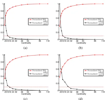
Fig. 1. The average IRQ of all subjects versus cardinality (a)
OS, (b) BE, (c) RWE and (d) FS. The red line is the 10 percent threshold that determines the optimum cardinality to be used in the test data. The optimum cardinality levels for OS, BE, RWE and FS methods are 10, 10, 16 and 24 respectively.
we computed the corresponding RQ value. We studied the RQ curve and determined the optimal cardinality where its value suddenly dropped indicating we started to lose infor-mative channels.
The EEG dataset contains 140 trials per class and subject. We used a 4-fold cross validation technique. We divided the data into 4 folds where each of the folds contains 35 trials per class. We used each fold for extracting the spatial filter and training the classifier. The learned system is tested on the rest of the data. The results obtained from four folds are averaged to obtain the final accuracy of the interested method.
3. RESULTS
In order to determine the optimal cardinality level to be used on the test data, the RQ values related to each cardinality level were computed on the training data, scaled to their maximum value and averaged over subjects. In the following step, we computed the slope of the RQ curve and normalized it to its maximum value to get an idea about the relative change in the RQ.
We depicted the change in RQ values for each cardinality as shown in Fig. 1. As expected, decreasing the cardinality of the spatial projection resulted to a decrease in the RQ value. To determine the optimum cardinality to be used in classifica-tion on the test data, we selected the cardinality that is closest to 10% of the maximum relative change (dashed lines in Fig.
2 5710 16 24 32 48 64 96 118 5 10 15 20 25 30 Cardinality Classification Error(%) Oscillating Search Backward Elimination Recursive Weight Elimination Forward Selection
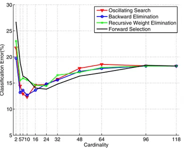
Fig. 2. The classification error curves of all methods versus
the cardinality. The last data point corresponds to the results obtained from standard CSP which uses all channels. 1). For BE and OS methods, the cardinality value was found to be 10 and for the FS and RWE methods, it was found to be 16 and 24, respectively. These indices perfectly corresponded to the elbow of the RQ curve, which indicates loss of infor-mative channels. In Table 1, we provided the classification re-sults and selected cardinalities for the EEG data set using each method. In order to give a sense of the change in error rate versus the cardinality, we provided the related classification error curves in Fig. 2. Although the minimum classification error was obtained at cardinality 24 for the RWE method, we noticed that we identified the optimum cardinality as 16 on the training data.
On all subjects we studied, we observed that the sparse spatial filter methods consistently outperformed the CSP method. We noted that the minimum error rate was obtained with OS method. Both OS and BE methods used cardinal-ity of 10 to achieve the minimum error rate. For the RWE method the optimum cardinality was 16 where for the FS method it was highest, 24. As expected the full CSP solution did not perform as good as the other sparse methods and
Table 1. EEG dataset classification error rates (%) for each
subject using LDA classifier
Cardinality aa al av aw ay Avg OS 10 21.1 3.57 22.3 7.68 6.96 12.3 BE 10 21.1 3.21 24.3 8.57 6.25 12.7 RWE 16 22.1 3.39 28.8 8.93 9.64 14.6 FS 24 20.2 3.21 29.3 8.75 7.68 13.8 CSP 118 27.9 5.54 34.3 10.9 12.7 18.2 aa al av aw ay Hand CSP F oot CSP Hand OS F oot OS
-0 +Fig. 3. The OS and CSP filters for hand and foot movement
imagination.
likely overfitted the training data. The OS method improved the classification error rate with an error difference of 5.9%. We obtained comparable results using the OS and BE meth-ods (p-value= 0.5, paired t-test) and comparable number of channels (p-value= 0.52).
Fig. 3 illustrates the distribution of the spatial filters ob-tained using the OS and CSP algorithms for each subject. We observed that the OS filter coefficients are localized on the left hemisphere and the central area except subject aa for foot filters, which is in accordance with the cortical regions related to right hand and the foot movement generation.
2 57 10 16 24 32 48 64 96 0 5 10 15 20 25 30 Cardinality Seconds Oscillating Search Backward Elimination Recursive Weight Elimination Forward Selection
Fig. 4. The average elapsed time to estimate a spatial filter vs.
the cardinality.
In order to compare the computational complexity of the methods, we measured the elapsed time for the
extrac-tion of a spatial filter from EEG data with cardinalities of
𝑘 ∈ {96, 64, 48, 32, 16, 10, 7, 5, 2}. The training was
per-formed on a regular desktop computer with 3 GB of RAM and equipped with a CPU running at 2.66 GHz. The elapsed time per filter computation decreased for the BE and RWE method and increased for the OS and FS method with the cardinality as shown in Fig. 4. The OS started with the computational time comparable to the FS and RWE at the beginning while it had the better results than them. OS was 20 times faster than the BE and better results than the BE at cardinality 10.
4. CONCLUSION
Recording systems containing large numbers of channels cause the CSP algorithm to overfit training data and to de-crease its generalization capability. To tackle with this prob-lem, we adapted the oscillating search method which fuses recently introduced greedy sparse filter selection methods such as BE, FS and RWE. We applied these sparse spatial fil-ter extraction methods, as well as traditional CSP, to the EEG data IVa of BCI competition IV that involves either right hand or foot imagined movements recorded from 5 subjects over 118 channels. We observed that the OS is more accurate than all other methods and reaches the minimum classification error by using sparse filters with cardinality as low as 10. Similar classification accuracies were obtained with the BE method with the same cardinality level. However, the average filter extraction time of the OS method is 20-times faster than the BE, making OS a more feasible technique in real-life applications which require rapid training stages.
5. REFERENCES
[1] B. Blankertz, R. Tomioka, S. Lemm, M. Kawanabe, and K.-R. M¨uller, “Optimizing spatial filters for robust EEG single-trial analysis,” Signal Processing Magazine,
IEEE, vol. 25, no. 1, pp. 41 –56, 2008.
[2] Nuri F. Ince, Rahul Gupta, Sami Arica, Ahmed H. Tew-fik, James Ashe, and Giuseppe Pellizzer, “High ac-curacy decoding of movement target direction in non-human primates based on common spatial patterns of local field potentials,” PLoS ONE, vol. 5, no. 12, pp. e14384, December 2010.
[3] H. Ramoser, J. M¨uller-Gerking, and G. Pfurtscheller, “Optimal spatial filtering of single trial EEG during imagined hand movement,” IEEE Transactions on
Re-habilitation Engineering, vol. 8, no. 4, pp. 441–446,
De-cember 2000.
[4] J. Farquhar, N. J. Hill, T. N. Lal, and B. Schlkopf, “Reg-ularised CSP for sensor selection in BCI,” in In
Proceed-ings of the 3rd International Brain-Computer Interface Workshop and Training Course, 2006.
[5] Xinyi Yong, R.K. Ward, and G.E. Birch, “Sparse spa-tial filter optimization for EEG channel reduction in brain-computer interface,” in Acoustics, Speech and
Sig-nal Processing, 2008. ICASSP 2008. IEEE InternatioSig-nal Conference on, April 2008, pp. 417 –420.
[6] M. Arvaneh, Cuntai Guan, Kai Keng Ang, and Chai Quek, “Optimizing the channel selection and classifi-cation accuracy in EEG-based BCI,” Biomedical
Engi-neering, IEEE Transactions on, vol. 58, no. 6, pp. 1865
–1873, June 2011.
[7] F. Goksu, N.F. Ince, and A.H. Tewfik, “Sparse com-mon spatial patterns in brain computer interface ap-plications,” in Acoustics, Speech and Signal
Process-ing (ICASSP), 2011 IEEE International Conference on,
May 2011, pp. 533 –536.
[8] Fikri Goksu, Firat Ince, and Ibrahim Onaran, “Sparse common spatial patterns with recursive weight elimi-nation,” in Signals, Systems and Computers
(ASILO-MAR), 2011 Conference Record of the Forty Fifth Asilo-mar Conference on, November 2011, pp. 117 –121.
[9] K-R Mueller B. Blankertz C. Sannelli, C. Vidaurre, “CSP patches: an ensemble of optimized spatial filters. an evaluation study.,” Journal of Neural Engineering, vol. 8(2):025012, pp. 7pp, 2011.
[10] T.N. Lal, M. Schroder, T. Hinterberger, J. Weston, M. Bogdan, N. Birbaumer, and B. Scholkopf, “Sup-port vector channel selection in bci,” Biomedical
Engi-neering, IEEE Transactions on, vol. 51, no. 6, pp. 1003
–1010, June 2004.
[11] P. Somol, J. Novovicov´a, J. Grim, and P. Pudil, “Dy-namic oscillating search algorithm for feature selec-tion,” in Pattern Recognition, 2008. ICPR 2008. 19th
International Conference on. IEEE, 2008, pp. 1–4.
[12] P. Somol and P. Pudil, “Oscillating search algorithms for feature selection,” in Pattern Recognition, 2000.
Proceedings. 15th International Conference on. IEEE,
2000, vol. 2, pp. 406–409.
[13] Guido Dornhege, Benjamin Blankertz, Gabriel Cu-rio, and Klaus-Robert M¨uller, “BCI competion iii, dataset iva,” 2005, http://www.bbci.de/ competition/iii/desc_IVa.html.
[14] B. Blankertz, K.-R. M¨uller, D.J. Krusienski, G. Schalk, J.R. Wolpaw, A. Schlogl, G. Pfurtscheller, Jd.R. Mill´an, M. Schr¨oder, and N. Birbaumer, “The BCI competition III: validating alternative approaches to actual BCI prob-lems,” Neural Systems and Rehabilitation Engineering,
IEEE Transactions on, vol. 14, no. 2, pp. 153 –159, June
2006.
[15] Baback Moghaddam, Yair Weiss, and Shai Avidan, “Generalized spectral bounds for sparse lda,” in
Pro-ceedings of the 23rd international conference on Ma-chine learning, New York, NY, USA, 2006, ICML ’06,
pp. 641–648, ACM.
[16] Isabelle Guyon, Jason Weston, Stephen Barnhill, and Vladimir Vapnik, “Gene selection for cancer classifica-tion using support vector machines,” Machine Learning, vol. 46, no. 1-3, pp. 389–422, 2002.
[17] Lester Mackey, “Deflation methods for sparse PCA,” in Advances in Neural Information Processing Systems
21, D. Koller, D. Schuurmans, Y. Bengio, and L. Bottou,
Eds., pp. 1017–1024. 2009.
[18] Richard O. Duda, Peter E. Hart, and David G. Stork, Pattern Classification (2nd Edition), Wiley-Interscience, 2000.