DOI: 10.1002/nbm.4228
R E S E A R C H A R T I C L E
Factorized sensitivity estimation for artifact suppression in
phase-cycled bSSFP MRI
Erdem Bıyık
1,2,3Kübra Keskin
3,4Salman UH Dar
3,4Aykut Koç
2,3,4Tolga Çukur
3,4,51Department of Electrical Engineering,
Stanford University, CA, USA
2Intelligent Data Analytics Research Program
Department, Aselsan Research Center, Ankara, Turkey
3Department of Electrical and Electronics
Engineering, Bilkent University, Ankara, Turkey
4National Magnetic Resonance Research
Center (UMRAM), Bilkent University, Ankara, Turkey
5Neuroscience Program at Sabuncu Brain
Research Center, Bilkent University, Ankara, Turkey
Correspondence
Tolga Çukur, Ph.D., Department of Electrical and Electronics Engineering, Room 304, Bilkent University, Ankara, TR-06800. Email: [email protected]
Funding information
Bilim Akademisi, Grant/Award Number: BAGEP 2017; European Molecular Biology Organization, Grant/Award Number: IG 3028; Türkiye Bilimler Akademisi, Grant/Award Number: GEBIP 2015; Türkiye Bilimsel ve Teknolojik Ara¸stirma Kurumu, Grant/Award Number: 117E171
Objective: Balanced steady-state free precession (bSSFP) imaging suffers from banding artifacts
in the presence of magnetic field inhomogeneity. The purpose of this study is to identify an efficient strategy to reconstruct banding-free bSSFP images from multi-coil multi-acquisition datasets.
Method: Previous techniques either assume that a naïve coil-combination is performed a priori
resulting in suboptimal artifact suppression, or that artifact suppression is performed for each coil separately at the expense of significant computational burden. Here we propose a tailored method that factorizes the estimation of coil and bSSFP sensitivity profiles for improved accuracy and/or speed.
Results: In vivo experiments show that the proposed method outperforms naïve coil-combination
and coil-by-coil processing in terms of both reconstruction quality and time.
Conclusion: The proposed method enables computationally efficient artifact suppression for
phase-cycled bSSFP imaging with modern coil arrays. Rapid imaging applications can efficiently benefit from the improved robustness of bSSFP imaging against field inhomogeneity.
KEYWORDS
balanced SSFP, banding artifact, artifact suppression, coil combination, sensitivity estimation, joint reconstruction
1
INTRODUCTION
Balanced SSFP is a rapid imaging sequence with broad use in many applications including angiography,1,2musculoskeletal imaging,3,4cardiac
imaging,5-7cell tracking,8,9interventional imaging,10,11and functional imaging.12,13However, its elevated sensitivity to magnetic field
inhomo-geneity causes signal voids in acquired images known as banding artifacts. This undesirable sensitivity can be alleviated by pulse sequence designs that modify off-resonance profiles,14-16 advanced field shimming procedures,17 or multi-acquisition phase-cycled bSSFP imaging.18
Multiple-acquisition bSSFP has remained a common choice since it demonstrates improved reliability against field inhomogeneity18,19and it can
additionally offer fat-water separation.20-22
In multi-acquisition bSSFP, several images with spatially nonoverlapping artifacts are jointly processed to yield an artifact-suppressed image. A common approach for suppression is to use heuristic combinations of voxel intensities such as maximum-intensity (MI), complex-sum (CS) and sum-of-squares (SOS).18,23,24For improved performance, more sophisticated combinations were later proposed including nonlinear averaging,25
Erdem Bıyık and Kübra Keskin contributed equally to this work.
Abbreviations: bSSFP, balanced steady state free precession; CCP, coil-by-coil processing; CS, complex-sum; CSF, Cerebrospinal fluid;
ESM, elliptical signal model; FBS, factorized banding suppression; MI, maximum-intensity; SOS, sum-of-squares; MRI, magnetic resonance imaging; PSNR, peak signal-to-noise ratio; ROI, region of interest; SBC, sensitivity based combination; TE, echo time; TR, repetition time.
NMR in Biomedicine. 2020;33:e4228. wileyonlinelibrary.com/journal/nbm © 2020 John Wiley & Sons, Ltd. 1 of 14
partial complex summation,26and p-norm.27These heuristic combinations are typically used when a limited number of acquisitions (N< 4) are
available.
Alternatively, the bSSFP signal model can be leveraged to estimate a banding-suppressed image. A structured method is LORE-GN that estimates tissue parameters by solving a nonlinear least-squares problem.28,29Although LORE-GN can work with down to N= 3, nonlinear
optimization can yield instability in high-signal regions. Later studies showed that the bSSFP signal follows an elliptical model across acquisitions, and proposed geometric and algebraic methods to estimate the ellipse parameters.30,31 Despite the improved stability, methods based on
the elliptical signal model require at least N ≥ 4for reliable performance. This requirement is equally valid for recent techniques based on dictionary-based estimation32and multilayer perceptron-based (MLP) learning.33We also note several studies with the purpose of decreasing
data acquisition time and/or the required number of phase-cycles for elliptical signal model34-36; however reliable banding suppression with N< 4
remains a challenging task.
Previous artifact suppression methods primarily focused on data combination across the acquisition dimension. In naïve coil-combination, coil sensitivites are estimated on images with banding artifacts and coil combination is then performed independently for each acquisition, leading to suboptimal artifact suppression. Meanwhile, computational burden can be elevated for coil-by-coil processing that performs acquisition combination on each coil separately, and for joint processing that performs simultaneous acquisition-coil combination. Here we propose an improved method based on factorized combination across the coil and acquisition dimensions. To prevent bias in coil sensitivity estimates due to bSSFP profiles,37the proposed method first performs a phase-preserving acquisition combination. Coil sensitivities are then estimated from
the combined data via an eigen-decomposition approach,38and used to linearly combine multi-coil multi-acquisition data across coils. Lastly, a
banding-suppressed image is obtained using an acquisition combination tailored to N. Comprehensive experiments are presented to demonstrate the computational efficiency and reliability of the proposed method in artifact suppression compared to previous techniques.
2
THEORY
In this paper, we consider the joint encoding model for multi-coil, multi-acquisition bSSFP images used in Ref.37The joint encoding model casts
the bSSFP image captured by the dthcoil element in the nthphase-cycled acquisition as:
Sn,d(r) = Pn(r)Cd(r)So(r) (1)
where r is the spatial location. Pndenotes the bSSFP sensitivity profile of the nthacquisition39; and Cddenotes the coil sensitivity profile of the d th coil element. Sodenotes a target bSSFP image, with no spatial modulations due to coil or bSSFP sensitivity profiles (i.e., center of the passband contrast assumed across the entire field-of-view). In theory, Socan be inferred given multi-acquisition multi-coil data Sn,d.
Methods that aim to suppress banding artifacts in bSSFP images essentially try to estimate So(r)given Sn,d(r). The widely adopted practice for multi-coil datasets is to first perform coil combination with estimated sensitivities40:
̂Cn,d(r) = ⟨Sn,d
(r)⟩ √∑D
i=1|⟨Sn,i(r)⟩|2
(2)
where⟨⟩denotes a low-spatial-frequency image reconstructed from central k-space data assuming that coil sensitivities vary smoothly, the total number of coils is D and number of phase-cycled acquisitions is N. Based on estimated coil sensitivities, the SNR-optimal coil combination for each acquisition is:
Sc n(r) = D ∑ d=1 Sn,d(r) ̂C∗ n,d(r) ∑D i=1| ̂Cn,i(r)|2 (3) where∗denotes the complex-conjugate operation.
The performance of coil combination depends on the accuracy of the denominator in Equation (2). However, the SOS combination in the denominator can show signal inhomogeneity that leaks onto final bSSFP images. Furthermore, naïve coil-sensitivity estimation does not consider spatial modulations due to bSSFP profiles, so naïve estimates are typically biased. Despite these limitations, the standard approach is to process coil-combined datasets (Sc
n(r)) to suppress banding artifacts. In the following subsections, we first summarize previous artifact suppression techniques including intensity-, sensitivity- and model-based methods. We then introduce the proposed method.
2.1
Intensity-Based Combination
A popular approach for artifact suppression in multi-acquisition bSSFP imaging is to perform voxel-wise combination of image intensity across acquisitions. Intensity-based methods do not take into account the underlying bSSFP signal model, hence they can yield suboptimal performance. However, these methods work even for relatively small number of acquisitions (N ≥ 2), and they offer efficient computation. Among common intensity-based methods are MI, SOS, P-norm, and CS. MI enhances artifact suppression, SOS yields near-optimal SNR, and P-norm offers a desirable trade-off between the two (here we use p= 4for the P-norm). Unlike these phase-insensitive methods, CS retains image phase at the expense of signal cancellations.
Other heuristic combination techniques are modifications of the above-mentioned methods. We refer to Ref.25for nonlinear averaging and to
Ref.26for partial complex summation methods, both of which reduce to MI for N= 2. For brevity, we do not report these techniques in this study.
2.2
Sensitivity-Based Combination (SBC)
An alternative to intensity-based combination is a weighted combination of multiple acquisitions where the weights are proportional to the bSSFP sensitivity profiles. In sensitivity-based combination, data-driven estimates of bSSFP profiles are obtained from phase-cycled bSSFP images without explicit use of analytical signal equations.22Here the ESPIRiT method was used for estimation with the assumption that bSSFP
sensitivites show gradual spatial variation.38These estimates,̂P
n(r), are then used for combination:
̂So(r) = N ∑ n=1 Sc n(r) ̂P∗n(r) ∑N i=1|̂Pi(r)|2 (4)
In principle, a combination can also be performed using joint sensitivity profiles across coil and acquisition dimensions, Jn,d(r) =Pn(r)Cd(r):
̂So(r) = N ∑ n=1 D ∑ d=1 Sn,d(r)̂J∗ n,d(r) ∑N i=1 ∑D j=1|̂Ji,j(r)|2 (5)
Regardless of whether SBC is performed on coil-combined images or jointly across coils and acquisitions, residual inhomogeneities can bias sensitivity estimates and result in suboptimal artifact suppression.
2.3
Combination Based on the Elliptical Signal Model (ESM)
In contrast to SBC, model-based combination leverages an explicit analytical model of the bSSFP signal. Here we specifically consider the elliptical signal model (ESM).30To estimate a banding-suppressed image, ESM starts by observing the analytical signal model:
Sc
n(r) = M(r)
1 − A(r)e−j(𝜙(r)+Δ𝜙n)
1 − B(r) cos(𝜙(r) + Δ𝜙n)
(6)
where M, A, and B are independent of𝜙(r) +𝛥𝜙n, and only depend on sequence and tissue parameters;𝜙(r)is phase accrued in a TR due to field inhomogeneity; and𝛥𝜙nis the phase increment of nthphase-cycle.
GivenSc
nat N distinct increments for a voxel, ESM attempts an inverse problem to estimate the banding-free component of the bSSFP signal. Specifically, ESM leverages the elliptical distribution of phase-cycled bSSFP signals in the complex plane.30To estimate the banding-free
signal, the first pass solution is to identify the ellipse's cross-point and the second-pass solution is to do a weighted combination across a spatial neighborhood of voxels. For single-coil or coil-combined acquisitions, ESM typically outperforms intensity- and sensitivity-based combinations when N = 4 phase-cycled acquisitions are available. However, the best strategy for performing ESM on multi-coil acquisitions remains unclear.
The original paper proposed ESM as a method for N= 4. Higher number of phase-cycles are also used in both research32,33,37,41,42 and
practice.43,44In this paper, we simply extend ESM to N= 8in the following way. We perform ESM combination over all feasible subsets of 4
phase-cycles and then take the average of the resulting images for denoising. A feasible set of 4 phase-cycles means there are two pairs, and within each pair phase-cycles have a phase difference of𝜋.
3
METHODS
3.1
Factorized Banding Suppression
Previous approaches for banding suppression in multi-coil datasets commonly perform a coil-combination on each acquisition independently. This naïve coil combination requires estimation of coil sensitivities from a set of images that carry additional spatial modulation from bSSFP profiles. Thus sensitivity estimates can be biased, resulting in suboptimal artifact suppression. While individual coils can instead be processed separately, substantial computational burden is introduced.
To achieve reliable and computationally efficient artifact suppression, here we propose a new method, factorized banding suppression (FBS) that initially performs a complex-summation across acquisitions to suppress modulations due to bSSFP profiles in multi-coil images:
Sa d(r) = N ∑ n=1 Sn,d(r) (7)
Here the complex-sum combination is preferred since it retains phase information such that subsequent acquisition combination can be performed on complex data. The intermediate multi-coil acquisition-combined images,Sa
d, are then used to estimate a shared set of coil sensitivities for all acquisitions.
Since sensitivity estimates based on Equation (2) can yield residual signal inhomogeneity, FBS employs a reference-free estimation approach based on the eigenvalue formulation cast by the ESPIRiT method.38 Given stacked multi-coil acquisition-combined images
Sa(r) = [Sa 1(r) S a 2(r) … S a D(r)], a self-consistency constraint 45is imposed: [ −1 c ] rS a(r) = Sa(r) (8)
whereis the Fourier operator, andcis a convolution operator estimated from central k-space data and expressed as a positive semidefinite matrix.38 In this formulation, Sa is an eigenvector of
−1
c with the eigenvalue 1. Since Sa(r) = [So(r)C1(r)So(r)C2(r) …So(r)CD(r)], the coil sensitivities are also eigenvectors at spatial locations:
[ −1
c
]
rC(r) = C(r) (9)
where C(r) = [C1(r)C2(r) …CD(r)]and So(r)≠ 0. Solution of Equation (9) thereby yields explicit estimates of coil sensitivities.
Once a consistent set of coil sensitivities, ̂Cd, are obtained from acquisition-combined data, the original multi-coil multi-acquisition data are optimally combined: Sc n(r) = D ∑ d=1 Sn,d(r) ̂C∗ d(r) ∑D i=1| ̂Ci(r)|2 (10) whereSc
n(r)denotes the coil-combined image for the nthacquisition. The final step is to perform acquisition combination onScnto obtain a banding-suppressed reconstruction̂So.
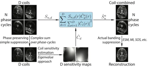
FBS factorizes the estimation of ̂So into two subproblems where enhanced coil sensitivity estimates are obtained following an initial phase-preserving acquisition combination, and then artifact suppression is achieved on the resultant coil-combined acquisitions (Figure 1). Since it requires a single CS combination over N acquisitions, coil-sensitivity estimation for D coils, and a final acquisition combination over N images, FBS offers improved computational efficiency compared to coil-by-coil processing.
Here we implemented several variants of FBS based on intensity-, sensitivity- and model-based combinations. For N< 4, all variants were compared except ESM that is inapplicable. Since we observed FBS-MI to outperform alternatives in this case, for N ≥ 4comparisons were restricted to FBS-MI and FBS-ESM. For FBS-SBC, bSSFP sensitivity profiles were estimated using a self-consistency formulation analogous to estimation of coil sensitivities.39,46Once estimated, these sensitives were used to combine acquisitions as in Equation (4).
3.2
Alternative Methods
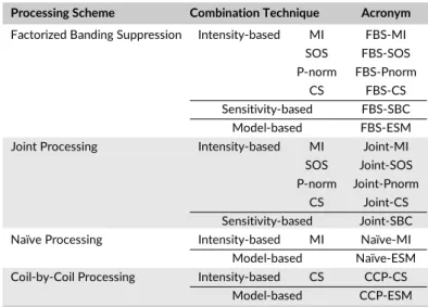
Three alternative approaches to FBS were considered: joint combination across coils and acquisitions, naïve coil combination followed by acquisition combination, and coil-by-coil processing. The full list of banding suppression methods tested here is given in Table 1 with their acronyms for convenience.
3.2.1 Joint Processing
Combination was performed simultaneously across the coil and acquisition dimensions. Intensity- and sensitivity-based combinations were implemented. For intensity-based combination, variants based on MI, SOS, p-norm and CS were used (i.e., Joint-MI, Joint-SOS etc.), where a joint combination was performed over coils and acquisitions. For sensitivity-based combination, joint sensitivity profiles across coils and acquisitions
FIGURE 1 Flowchart of the proposed factorized-banding-suppression (FBS) method for multi-coil multi-acquisitions bSSFP datasets. To prevent bias in coil sensitivity estimation, FBS first performs a phase-preserving acquisition combination. An eigenvalue formulation is cast to estimate a consistent set of coil sensitivities from these acquisition-combined multi-coil data. The original multi-coil multi-acquision data are then optimally combined across the coil dimension based on the estimated sensitivities. Finally, banding artifacts are effectively suppressed by combining multiple acquisitions using a method tailored to the number of acquisitions (e.g., maximum-intensity for N< 4, elliptical signal modeling for N ≥ 4)
Processing Scheme Combination Technique Acronym Factorized Banding Suppression Intensity-based MI FBS-MI
SOS FBS-SOS P-norm FBS-Pnorm
CS FBS-CS
Sensitivity-based FBS-SBC Model-based FBS-ESM Joint Processing Intensity-based MI Joint-MI
SOS Joint-SOS P-norm Joint-Pnorm
CS Joint-CS Sensitivity-based Joint-SBC Naïve Processing Intensity-based MI Naïve-MI Model-based Naïve-ESM Coil-by-Coil Processing Intensity-based CS CCP-CS
Model-based CCP-ESM
TABLE 1 List of Banding Suppression Methods in this Study
were initially estimated via ESPIRiT as described in Ref.37After estimation of joint sensitivities (̂J
n,d), we used the optimal linear combination described in Equation (5) to obtain a banding-suppressed imagêSo(Joint-SBC). Note that ESM does not explicitly consider the coil dimension, so no variants were considered based on model-based combination.
3.2.2 Naïve Processing
Coil combination was performed based on coil sensitivities estimated for each acquisition independently, and an acquisition combination followed. Here we estimated coil sensitivities following the procedure described in Equation (9) to obtain coil-combined imagesSc
nas in Equation (10). Several variants were implemented that combined acquisitions based on intensity-, sensitivity- and model-based methods. It was observed that Naïve-MI outperforms other variants at N= 2, thus for N ≥ 4only Naïve-MI and Naïve-ESM were tested. Note that sensitivity estimation can be computationally demanding for large N and D due to the size of the eigenvalue problem in Equation (9).
3.2.3 Coil-by-Coil Processing (CCP)
Multi-acquisition data for each coil were first processed to suppress banding artifacts. The resulting coil imageŝSa
dwere then combined as in Equation (3). Note that acquisition combination methods that discard phase information would prevent accurate estimation of coil sensitivities in the subsequent step. Thus, only two variants CCP-CS and CCP-ESM (for N ≥ 4) were considered. CCP requires acquisition combination to be repeated D times on N acquisitions, resulting in added computational burden compared to FBS.
4
SIMULATIONS
Simulation-based analyses were performed to identify optimal parameters in ESPIRiT for accurate estimation of coil and bSSFP sensitivity profiles. ESPIRiT observes that correlations across k-space samples are encoded in the null space of a matrix formed from calibration data, and that sensitivity profiles can be estimated as the main eigenvector of a reconstruction operator obtained from this null space.38 The null
space is computed via singular value decomposition of the calibration matrix. To improve sensitivity, a threshold (𝜎2
cut-off) with respect to the
maximum singular value is applied to mask out components with small singular values. As such, estimation of coil and bSSFP sensitivity profiles involves selection of three parameters in ESPIRiT: the calibration region size, the kernel size and the cut-off value. Here, three types of profile estimation was performed: coil sensitivities, bSSFP sensitivities, and joint coil-bSSFP sensitivities. Parameter selection was performed for each type separately.
Parameters were selected based on reconstructions of a simulated two-dimensional (2D) brain phantom. Simulations were performed at 0.5 mm isotropic resolution,60◦flip angleΔ𝜙 = 2𝜋[0∶1∶(N−1)]N with N= 8, and TR/TE=10.0∕5.0ms where TE is the echo time. Bivariate Gaussian noise was added to simulated images to achieve an acquisition SNR of 20 for CSF tissue, where SNR was taken as the ratio of signal intensity to standard deviation of noise. A main-field inhomogeneity yielding0±62Hz (mean±std across volume) off-resonance, and an array of D= 8
coils arranged in a circular configuration were assumed.47Tissue parameters were adapted from Ref.37:3000∕1000ms for CSF,1200∕250ms
for blood,1000∕80ms for white matter,1300∕110ms for gray matter,1400∕30ms for muscle, and370∕130ms for fat.
For coil-sensitivity estimation, the following parameter values were examined: calibration region size∈ [6.6%, 12.8%](indicating the area of the calibration region in proportion with the area of the entire k-space grid), kernel size∈ [5, 13](in units of number of k-space samples), and
𝜎2
cut-off∈ [10
−3, 1). A banding-free bSSFP image (i.e., with center of the passband contrast across the FOV) was simulated and multiplied with
known coil sensitivities for D= 8. Coil-sensitivities were estimated from multi-coil phantom images via ESPIRiT; and a coil-combined bSSFP image was obtained using the sensitivity estimates. Ideally, the coil-combined bSSFP image should be identical to the original banding-free bSSFP
image. Thus, reconstruction quality was taken as peak signal-to-noise ratio (PSNR) between the reconstructed and original bSSFP images. PSNR was calculated in dB as follows:
PSNR = 10log10 1 1 R ∑R r=1(|̂So(r)| − |Sref(r)|)2 (11)
where the denominator denotes mean-squared error between the reconstructed (̂So(r)) and reference (Sref(r)) images, R denotes the number of voxels, and the maximum signal intensity is assumed to be 1. The results across the tested range of parameters are shown in Figure 2A.
For bSSFP and joint coil-bSSFP sensitivity estimations, the following parameter values were examined: calibration region size∈ [16%, 68%], kernel size∈ [9, 37], and𝜎2
cut-off∈ [0.001, 0.256]. Multi-coil phase-cycled bSSFP images were simulated for D= 8, N= 8. Sensitivity estimates
were again obtained via ESPIRiT, and then used to combine multi-coil bSSFP images. Reliability of the sensitivity estimates was assessed by calculating the level of residual banding artifacts in the combined image. The artifact level was taken as the standard deviation of the signal magnitude over an ideally homogeneous region of interest (ROI). Since measurementswere over-sensitive to noise in gray and white matter, artifact levels in CSF ROIs (𝜎csf) were considered for parameter selection. The results across the tested range of parameters are shown in Fig. 2B,C.
The selected parameters for each type of profile were thereafter used in estimations of the same type, regardless of the reconstruction method.
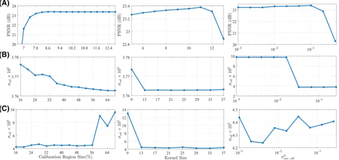
FIGURE 2 Coil and bSSFP sensitivity profiles are estimated using central k-space data based on three parameters: the calibration region size, the kernel size and the cut-off value for eigenvalues. All parameters were selected to optimize the quality of coil- and acquisition-combinations during reconstructions of a numerical brain phantom. Reconstruction quality was measured as peak signal-to-noise ratio (PSNR) between the reconstruction and an ideal reference image. Level of residual banding artifacts was measured as the standard deviation of signal intensity across an ideally uniform region of CSF tissue (𝜎csf). A, Measurements for coil combination as in Equation (3). A relative calibration region size of9%,
kernel size of 11 and𝜎2
cut-off= 0.1yield optimal performance for coil combination. B, Measurements for acquisition combination as in
Equation (4). A calibration region size of64%, kernel size of 13 and𝜎2
cut-off= 0.032yield optimal performance for acquisition combination.
C, Measurements for joint combination across coils and acquisitions as in Equation (5). A calibration region size of20%, kernel size of 33 and
𝜎2
cut-off= 0.004yield optimal performance for joint combination. Note that, for all cases, near-optimal performance is attained for a broad range
of values across the optimum values listed above
FIGURE 3 Phase-cycled bSSFP acquisitions of a homogeneous phantom were performed with D=32 (Dataset #1). A, Individual acquisitions are displayed after combination across the coil dimension. B, Acquisitions with N∈{4,8} were reconstructed using the ESM-variants of Naïve, CCP and FBS methods.
5
EXPERIMENTS
Four different datasets were prepared in order to demonstrate the performance and computational efficiency of FBS framework. All acquisitions were performed on a 3T whole-body scanner (Siemens Magnetom Trio, Ankara, Turkey) with gradients (a maximum strength of 45 mT/m and a maximum slew rate of 200 T/m/s). A 3D Cartesian bSSFP sequence was prescribed with a flip angle of30◦, a field-of-view of 218 mm, elliptical scanning, and N= 8separate acquisitions with𝛥𝜙spanning[0, 2𝜋)in equispaced intervals. Standard volumetric shimming was performed. Prior to each phase-cycled acquisition, a start-up segment with 10 dummy TRs was used to dampen transient signal oscillations. Acquisitions for each phantom or subject were collected sequentially without delay. Scan time per slice was 16.5 seconds for all datasets. A low readout bandwidth was used to increase acquisition SNR. The imaging protocols were approved by the local ethics committee at Bilkent University, and all participants gave written informed consent. The details that differ among datasets are summarized below:
• Dataset #1: bSSFP acquisitions of a homogeneous phantom with T1∕T2 ≈ 2were performed using a 32-channel head coil (D= 32) with a TR/TE of 8.08 ms/4.04 ms, a resolution of0.85 × 0.85 × 0.85mm3, a readout bandwidth of 201 Hz/pixel. (Please see Figure 3 for individual
phase-cycled bSSFP images of the phantom, and for reconstructions with various combination methods.)
• Dataset #2: In vivo bSSFP acquisitions of the brain from seven subjects were performed using a 12-channel head coil with a TR/TE of 8.08
ms/4.04 ms, a resolution of0.85×0.85×0.85mm3, a readout bandwidth of 199 Hz/pixel. The stock bSSFP sequences used in the experiments
performed automatic hardware compression to D= 4channels.
• Dataset #3: In vivo bSSFP acquisitions of the knee from a single subject were performed using a 15-channel knee coil (D= 15) with a TR/TE of 8.08 ms/4.04 ms, a resolution of0.85 × 0.85 × 0.85mm3, a readout bandwidth of 199 Hz/pixel.
• Dataset #4: In vivo bSSFP acquisitions of the brain from three subjects were performed using a 32-channel head coil (D= 32) with a TR/TE of 8.04 ms/4.02 ms, a resolution of0.85 × 0.85 × 3mm3, a readout bandwidth of 201 Hz/pixel.
In this work, we estimated coil sensitivities using an optimal linear combination, as formulated in Equation (2), following procedures in Ref.40A
reference image was obtained by performing FBS-ESM on bSSFP data acquired at N= 8(observed to yield the best artifact suppression here). To improve reliability against outliers, we performed remapping of voxel intensity values prior to PSNR measurements. The intensity values were first linearly transformed to map the1th− 99thpercentile to [0 1]. Values in [99 100]% were saturated to 1, and values in [0 1]% were set to 0.
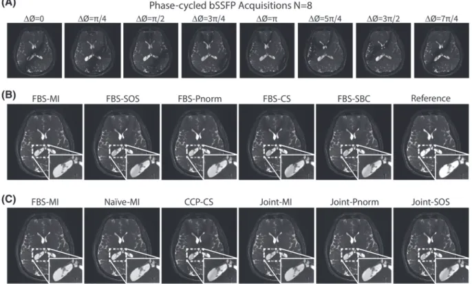
FIGURE 4 In vivo bSSFP acquisitions of the brain withD = 4, N = 2were reconstructed (Dataset #2). (a) Individual acquisitions are displayed after combination across the coil dimension. (b) Several variants of FBS were examined including intensity-based (MI, SOS, Pnorm, CS) and sensitivity-based (SBC) acquisition combination. A reference image obtained via FBS-ESM withN = 8is also shown. Residual banding artifacts are clearly visible in FBS-SOS, FBS-CS and FBS-SBC. In contrast, FBS-MI yields enhanced suppression with no visible artifacts, and PBS-Pnorm performs closely. (c) FBS-MI was compared against the alternative Naive, CCP and Joint methods. FBS-MI achieves superior artifact suppression with reconstruction that closely resemble the reference image. While Naïve-MI performs similarly, FBS-MI is computationally more efficient than Naïve-MI(see Table 4).
TABLE 2 PSNR,𝜎csf,𝜎gmand𝜎wmatN = 2 PSNR (dB) 𝜎csf 𝜎gm 𝜎wm FBS MI 25.1 ± 0.4 0.057 ± 0.009 0.024±0.001 0.015±0.001 SOS 25.2 ± 0.4 0.082 ± 0.014 0.026±0.002 0.023±0.001 P-norm 25.3 ± 0.4 0.066 ± 0.011 0.023±0.001 0.016±0.001 CS 24.5 ± 0.4 0.083 ± 0.014 0.032±0.002 0.028±0.002 SBC 25.0 ± 0.4 0.081 ± 0.014 0.026±0.002 0.023±0.002 Joint MI 24.5 ± 0.3 0.065 ± 0.010 0.027±0.001 0.016±0.001 SOS 25.0 ± 0.4 0.082 ± 0.014 0.026±0.002 0.023±0.001 P-norm 25.1 ± 0.4 0.070 ± 0.012 0.023±0.001 0.017±0.001 CS 19.0 ± 0.3 0.136 ± 0.020 0.051±0.006 0.033±0.003 SBC 25.0 ± 0.4 0.081 ± 0.014 0.026±0.002 0.023±0.002 Note. Measurements are reported as mean±se subjects.
TABLE 3 PSNR atN = 2, 4andD = 4, 32 PSNR (dB) D=4 N=2 Naïve-MI 25.0 ± 0.4 Joint-P-norm 25.1 ± 0.4 CCP-CS 24.5 ± 0.4 FBS-MI 25.1 ± 0.4 N=4 Naïve-ESM 26.7 ± 1.2 Joint-SOS 28.4 ± 0.5 CCP-ESM 31.0 ± 0.9 FBS-ESM 31.0 ± 0.9 D=32 N=2 Naïve-MI 26.3 ± 0.5 Joint-P-norm 26.3 ± 0.4 CCP-CS 26.1 ± 0.5 FBS-MI 27.9 ± 0.7 N=4 Naïve-ESM 27.8 ± 2.0 Joint-SOS 29.5 ± 0.3 CCP-ESM 36.0 ± 0.8 FBS-ESM 38.3 ± 0.3
Note. Measurements are reported as mean±se subjects at N = 2, 4 and D = 4, 32. Note that model-based combination (ESM) is not applicable at N = 2, so MI, CS and P-norm variants are considered instead. PSNR values were measured only for N = 2 and N = 4; because N = 8 was used for reference images.
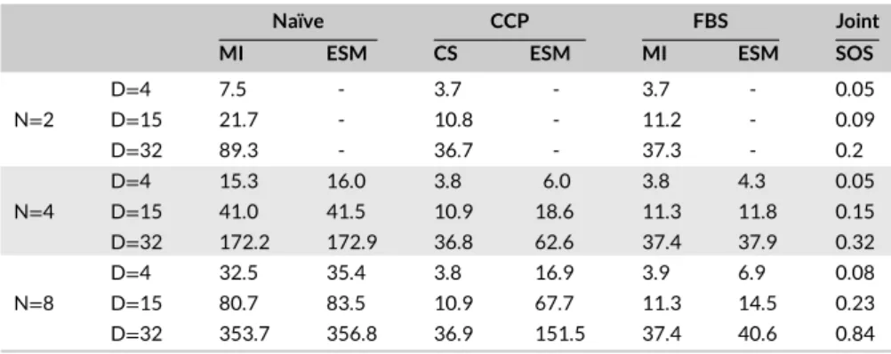
TABLE 4 Reconstruction Times (seconds)
of Naïve, CCP, FBS, and Joint Methods Naïve CCP FBS Joint
MI ESM CS ESM MI ESM SOS
D=4 7.5 - 3.7 - 3.7 - 0.05 N=2 D=15 21.7 - 10.8 - 11.2 - 0.09 D=32 89.3 - 36.7 - 37.3 - 0.2 D=4 15.3 16.0 3.8 6.0 3.8 4.3 0.05 N=4 D=15 41.0 41.5 10.9 18.6 11.3 11.8 0.15 D=32 172.2 172.9 36.8 62.6 37.4 37.9 0.32 D=4 32.5 35.4 3.8 16.9 3.9 6.9 0.08 N=8 D=15 80.7 83.5 10.9 67.7 11.3 14.5 0.23 D=32 353.7 356.8 36.9 151.5 37.4 40.6 0.84
Note. Average reconstruction times are reported for a single cross section at varying number of acquisitions N and number of coils D. Note that model-based combination (ESM) is not applicable at N = 2, so MI and CS variants are considered instead.
Reconstruction quality was then taken as PSNR between the reconstruction and the reference. The level of residual banding artifacts was taken as𝜎csfmeasured in the same cross-sections. Note that,𝜎csfanalysis was not performed on Dataset #4 as CSF region may contain signal variations
other than banding artifacts due to its thicker slices. The level of residual banding artifacts was also assessed for Gray Matter (𝜎gm) and White
Matter (𝜎wm). On average, the selected ROIs contained 379 62 voxels for CSF, 320 24 voxels for Gray Matter and 310 10 voxels for WhiteMatter
(mean se across subjects). Measurements were averaged across two central cross-sections within each subject. Significant differences among reconstructions were assessed with non-parametric Wilcoxon signed-rank tests.
Performance of combination methods were compared on Dataset #2 at N= 2. Reconstructions were obtained using the FBS, Joint, Naïve and CCP methods. For N= 4, 8; reconstructions were obtained using the ESM variants of the Naïve, CCP and FBS methods, and SOS variant of
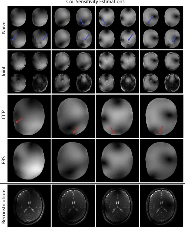
FIGURE 5 Coil sensitivities were estimated during Naïve, Joint, CCP and FBS reconstructions. Representative sensitivity maps for four of the coils are shown in Dataset #4 (D= 32) with N= 4, along with corresponding reconstructions for the same set of coils. The images displayed at the bottom row are individual-coil images that were combined across acquisitions obtained via the CCP method. Note that since sensitivity estimates are independently obtained for each phase-cycled acquisition in the Naïve method, it produces four separate estimates of a given coils sensitivity. Residual banding artifacts are clearly visible in the Naive method (marked with blue arrows), and residual tissue information leaks into the Joint method. In contrast, CCP and FBS are relatively immune to these issues. Close inspection further reveals that FBS yields smoother coil sensitivity estimates without abrupt transitions compared to CCP (marked with red arrows), especially near peripheral regions of the brain Joint method. We used Dataset #3 to demonstrate the performance of FBS in knee imaging; Dataset #2 and #4 to demonstrate the performance in brain imaging. Other than reconstructions, coil sensitivity map estimations were also produced within each method. Effects of different combination methods on coil sensitivity maps were demonstrated by using Dataset #4 for N= 4.
To assess computational efficiency, reconstructions of all datasets were performed using FBS, Naïve, CCP, and Joint methods. All cross-sections within volumetric datasets were reconstructed. Average computation times were recorded for varying number of acquisitions (N= 2, 4, 8) and number of coil elements (D= 4: the 12-channel head coil, D= 15: the 15-channel knee coil, D= 32, the 32-channel head coil). All analyses were executed in MATLAB (MathWorks, MA) on a workstation with Intel®Core™i7-6850 K CPU, 96 GB RAM.
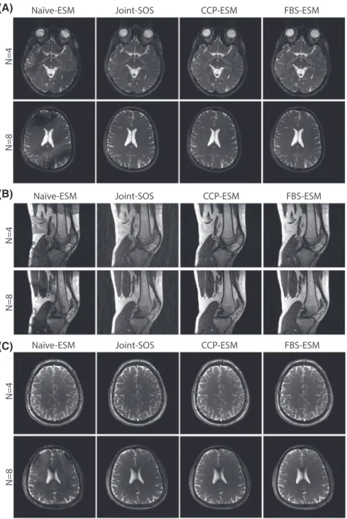
FIGURE 6 (a) In vivo bSSFP acquisitions of the brain were performed with
D = 4 (Dataset#2)(b) In vivo bSSFP acquisitions of the knee were performed withD = 15 (Dataset#3). (c) In vivo bSSFP acquisitions of the brain were performed withD = 32 (Dataset#4). In both cases, phase-cycled acquisitions withN = (4, 8) were reconstructed using the ESM variants of Naïve, CCP and FBS methods, and the SOS variant of Joint method. Representative reconstructions of separate cross-sections are shown. Biases in coil sensitivity estimates lead to substantial residual banding in
Naïve-ESM images; and Joint-SOS images show increased inhomogeneity in tissue signals. Meanwhile, FBS-ESM yields high-quality reconstructions. CCP-ESM performs similarly to FBS-ESM, yet FBS-ESM is significantly more efficient in terms of reconstruction time (see Table 4)
(A)
(B)
(C)
6
RESULTS
6.1
Analyses for N = 2
The proposed factorized banding suppression (FBS) method was first demonstrated for N < 4. In vivo bSSFP acquisitions of the brain for
N= 2and D= 4were reconstructed using the FBS, Joint, Naïve and CCP methods. Representative reconstructions from intensity-based and sensitivity-based variants of FBS are shown in Figure 4B. FBS-MI yields visibly superior artifact suppression compared to other variants, with FBS-Pnorm performing the second best. Reconstructions from Joint-MI, Joint-Pnorm, Joint-SOS, Naïve-MI and CCP-CS for the same dataset are displayed in Figure 4C. FBS-MI outperforms both Joint-SOS and CCP-CS methods, and it offers similar visual quality to Naïve-MI, Joint-MI and Joint-Pnorm reconstructions.
Quantitative comparisons of the FBS and Joint methods at N= 2are listed in Table 2 in terms of PSNR,𝜎csf,𝜎gmand𝜎wm. FBS yields better
results compared to the Joint method in terms of PSNR (p< 0.05) and𝜎csf(p< 0.05). For all variants, FBS produces 1.3 dB higher PSNR, 0.016
lower𝜎csf, 0.004 lower𝜎gm, and 0.002 lower𝜎wmthan the Joint method on average. This result indicates that FBS does not suffer from any
performance loss compared to joint processing of multi-coil, multi-acquisition datasets. Further comparisons focused on the best-performing variants of FBS, Naïve, Joint and CCP methods. PSNR measurements for FBS-MI againstNaïve-MI, Joint-Pnorm and CCP-CS are given in Table
3 forN = 2. Overall, FBS-MI yields significantly higher PSNR than all alternative methods(p< 0 ∶ 05), except Naïve-MI and Joint-Pnorm that perform similarly whenD = 4. For higher D, FBS-MI is significantly better than both Naïve-MI and Joint-Pnorm(p> 0.05), as indicated in Table 3. Also note that, even atN = 2andD = 4, FBS-MI is more computationally efficient than the Naïve method that requires separate coil sensitivity estimations for each acquisitions (see Table 4).
6.2
Analyses for N = 4 and N = 8
To examine potential biases in coil sensitivity estimation, coil sensitivity maps were obtained during Naïve, Joint, CCP and FBS reconstructions. Representative sensitivity map estimations are displayed in Figure 5 for D= 32and N= 4. Naïve suffers from clearly visible residual banding artifacts in sensitivity maps; Joint shows residual tissue information in sensitivity maps; and CCP yields some intensity shading near the peripheral regions of the brain. In contrast, FBS produces smoother and less biased coil sensitivity maps.
In vivo bSSFP acquisitions of the brain for N= 4, 8and D= 4, 32, and the knee for N= 4, 8and D= 15were reconstructed using Naïve-ESM, CCP-ESM, Joint-SOS and FBS-ESM. Representative reconstructions are displayed in Figure 6A for the brain(D = 4), in Figure 6B for the knee, and in Figure 6c for the brain(D = 32). For both anatomies, FBS achieves visually superior reconstruction quality compared to the Naïve and Joint methods, while FBS and CCP perform similarly.
These observations are confirmed with quantitative assessments of PSNR reported in Table 3 for the brain data. FBS-ESM and CCP-ESM yield higher performance than both Naïve-ESM and Joint-SOS atN = 4. As expected, the degraded performance of Naïve-ESM implies that biases in coil sensitivity estimates due to bSSFP profiles hamper the application of a model-based combination across acquisitions. Meanwhile, FBS yields similar reconstruction to CCP for (D= 4). Note that with the coils were readily hardware compressed to few channels, so the accuracy of coil sensitivity estimation is expected to be relatively limited in this case.
That said, differences in reconstruction quality between FBS and CCP emerged when the number of coils were higher. Our experiments with
D= 32clearly show that FBS yields significantly higher PSNR values than both Naïve, Joint and CCP methods for N= 2and N= 4(p< 0.05). Average PSNR values of the reconstructions over the subjects are presented in Table 3. For N= 2and N= 4respectively, FBS produces 1.6 and 10.5 dB higher PSNR than the Naïve method; 1.6 and 8.8 dB higher PSNR than the Joint method; and 1.8 and 2.3 dB higher PSNR than the CCP method.
FBS is also superior to both Naïve and CCP methods in terms of computational efficiency. Average reconstruction times for a single cross section are listed in Table 4 for N∈ {4, 8}and D∈ {4, 15, 32}. For ESM variants, FBS maintains up to 3.7 shorter processing time compared to CCP, and up to 8.8 times shorter processing time compared to Naïve. Note that Joint processing does not permit model-based combination, so an ESM variant could not be reported.While Joint-SOS can be computed fast in the absence of any sensitivity estimation, sensitivity-based variants were not reported either due to impractical reconstruction times.
7
DISCUSSION
A great deal of work has been done to date regarding artifact suppression methods in multi-acquisition phase-cycled bSSFP imaging. However, either single-coil acquisitions were considered, or a priori coil combination was performed for multi-coil datasets.48,49 Because naïve coil
combination of each acquisition creates biases in coil sensitivity estimates due to signal modulations from bSSFP sensitivity profiles, the performance of subsequent artifact suppression methods can be degraded. While a subset of existing methods can also be applied in a coil-by-coil fashion, a substantial computational burden is introduced for increasing numbers of acquisitions and coil elements.
Here, we proposed a factorized banding suppression (FBS) method that maintains reliable artifact suppression without compromising computational efficiency. Instead of estimating coil sensitivities separately for each acquisition, FBS uses a phase-preserving acquisition combination to obtain a consistent set of coil sensitivities. These estimates are used to combine images from multiple coils, and a subsequent acquisition combination is performed efficiently. The proposed method outperforms naïve coil combination in terms of the reliability of coil sensitivity estimates, and both naïve combination and coil-by-coil processing in terms of computational efficiency.
Computational efficiency of combination methods for multi-coil multi-acquision bSSFP datasets depend on both number of acquisitions (N) and number of coils (D) in addition to image size. Naive processing involves N×D coil sensitivity estimation, N combinations across coils, and 1 combination across acquisitions. Coil-by-coil processing involves D combinations across acquisitions, 1 coil sensitivity estimation, and 1 combination across coils. In ccontrast, FBS involves 2 combinations across acquisitions (the initial CS and subsequent combinations), 1 coil sensitivity estimation, and 1 combination across coils. Therefore, computational complexity of FBS is comparatively less dependent on N and D compared to naive processing and on D compared to CCP.
During this study, we also considered a neural-network-based method for artifact suppression in phase-cycled bSSFP datasets.33 When
number of acquisitions is limited (N< 4), we observed that FBS-MI outperforms a neural network even when trained on multiple coils and acquisitions jointly.33That said, further improvements in performance might be attained by using networks that directly allow complex-valued
mappings,50and deeper architectures trained on larger datasets. Furthermore, data augmentation methods, and transfer learning approaches,
where networks trained on different tissues are employed, might improve banding suppression performance. Hence, neural-network based methods is a promising avenue that warrants further investigation.
Subject motion can cause suboptimal performance in multi-acquisition phase-cycled bSSFP imaging due to several factors. First, regardless of the combination method, if uncorrected motion between separate acquisitions can lead to blurring and residual artifacts in the combined bSSFP image. Second, residual motion between acquisitions can also affect accuracy of methods that rely on estimates of coil or bSSFP sensitivity profiles. Naive processing is expected to show the greatest immunity to this issue since coil sensitivities are estimated independently for each acquisition. While joint processing simultaneously estimates coil and bSSFP sensitivities, no explicit constraint is used to enforce similariy of coil sensitivities across acquisitions, introducing some degree of reliability against motion. In contrast, CCP performs acquisition combination for individual coils prior to coil combination and FBS performs an initial complex-sum across acquisitions. These acquisition-combined images can contain residual artifacts, thereby introduce errors in subsequent coil-sensitivity estimation. When significant motion is present between acquisitions, a preprocessing stage could be incorporated prior to FBS to improve reliability.
Several modifications in FBS can be considered to yield improved performance. First, a complex summation was used here for the initial acquisition combination. While the CS method preserves phase information, it may yield suboptimal artifact suppression. To improve suppression, other phase-preserving combinations could be leveraged such as the complex version of the p-norm method.27Second, an initial acquisition
combination was performed here to estimate a common set of coil sensitivities across acquisitions. While this is a computationally efficient choice, accuracy of the estimates could be enhanced by using a tensor-based decomposition across the coil and acquisition dimensions of bSSFP datasets.37Lastly, the scan times for multi-acquisition bSSFP scans may prove to be impractical in applications with demanding requirements for
spatial resolution and coverage. To shorten scan times, acceleration methods such as compressed sensing could be employed51and FBS could
be used to combine the reconstructions.
In summary, FBS is an efficient method for combination of multi-coil multi-acquisition bSSFP datasets. The proposed method was primarily demonstrated for suppression of banding artifacts in phase-cycled bSSFP imaging. However, it can also benefit for other multi-acquisition applications where a priori coil-combination can improve computational efficiency such as fat-water separated or multi-echo bSSFP imaging.
ACKNOWLEDGMENTS
The authors would like to thank E. Ilıcak for his help with in vivo experiments, and E. Gündogdu for discussions on multilayer perceptron networks.̆ This work was supported in part by a Tubitak 1001 Research Grant (117E171), by a European Molecular Biology Organization Installation Grant (IG 3028), by a TUBA GEBIP 2015 fellowship, by a BAGEP 2017 fellowship, and by an NVIDIA GPU Grant awarded to T. Çukur.
ORCID
Tolga Çukur https://orcid.org/0000-0002-2296-851X
REFERENCES
1. Brittain JH, Olcott EW, Szuba A, et al. Three-dimensional flow-independent peripheral angiography. Magn Reson Med. 1997;38(3):343–354. 2. Cukur T, Lee JH, Bangerter NK, Hargreaves BA, Nishimura DG. Non-contrast-enhanced flow-independent peripheral MR angiography with balanced
SSFP. Magn Reson Med. 2009;61(6):1533–1539.
3. Hargreaves BA, Gold GE, Beaulieu CF, Vasanawala SS, Nishimura DG, Pauly JM. Comparison of new sequences for high-resolution cartilage imaging. Magn Reson Med. 2003;49(4):700–709.
4. Vasanawala SS, Hargreaves BA, Pauly JM, Nishimura DG, Beaulieu CF, Gold GE. Rapid musculoskeletal MRI with phase-sensitive steady-state free precession: comparison with routine knee MRI. Am J Roentgenol. 2005;184(5):1450–1455.
5. Peters DC, Ennis DB, McVeigh ER. High-resolution MRI of cardiac function with projection reconstruction and steady-state free precession. Magn Reson Med. 2002;48(1):82–88.
6. Jung BA, Hennig J, Scheffler K. Single-breathhold 3D-trueFISP cine cardiac imaging. Magn Reson Med. 2002;48(5):921–925.
7. Nayak KS, Hargreaves BA, Hu BS, Nishimura DG, Pauly JM, Meyer CH. Spiral balanced steady-state free precession cardiac imaging. Magn Reson Med. 2005;53(6):1468–1473.
8. Heyn C, Bowen CV, Rutt BK, Foster PJ. Detection threshold of single SPIO-labeled cells with FIESTA. Magn Reson Med. 2005;53(2):312–320. 9. Cukur T, Yamada M, Overall WR, Yang P, Nishimura DG. Positive contrast with alternating repetition time SSFP (PARTS): A fast imaging technique
for SPIO-labeled cells. Magn Reson Med. 2010;63(2):427–437.
10. Bieri O, Patil S, Quick HH, Scheffler K. Morphing steady-state free precession. Magn Reson Med. 2007;58(6):1242–1248.
11. Koktzoglou I, Li D, Dharmakumar R. Dephased FLAPS for improved visualization of susceptibility-shifted passive devices for real-time interventional MRI. Phys Med Bio. 2007;52(13):N277.
12. Scheffler K, Seifritz E, Bilecen D, et al. Detection of BOLD changes by means of a frequency-sensitive trueFISP technique: preliminary results. NMR Biomed. 2001;14(7-8):490–496.
13. Miller KL, Hargreaves BA, Lee J, Ress D, Christopher deCharms R, Pauly JM. Functional brain imaging using a blood oxygenation sensitive steady state. Magn Reson Med. 2003;50(4):675–683.
14. Nayak KS, Lee HL, Hargreaves BA, Hu BS. Wideband SSFP: alternating repetition time balanced steady state free precession with increased band spacing. Magn Reson Med. 2007;58(5):931–938.
15. Sun H, Fessler JA, Noll DC, Nielsen JF. Balanced SSFP-like steady-state imaging using small-tip fast recovery with a spectral prewinding pulse. Magn Reson Med. 2016;75(2):839–844.
16. Benkert T, Ehses P, Blaimer M, Jakob PM, Breuer FA. Dynamically phase-cycled radial balanced SSFP imaging for efficient banding removal. Magn Reson Med. 2015;73(1):182–194.
17. Lee J, Lustig M, Kim Dh, Pauly JM. Improved shim method based on the minimization of the maximum off-resonance frequency for balanced steady-state free precession (bSSFP). Magn Reson Med. 2009;61(6):1500–1506.
18. Bangerter NK, Hargreaves BA, Vasanawala SS, Pauly JM, Gold GE, Nishimura DG. Analysis of multiple-acquisition SSFP. Magn Reson Med. 2004;51(5):1038–1047.
19. Quist B, Hargreaves BA, Cukur T, Morrell GR, Gold GE, Bangerter NK. Simultaneous fat suppression and band reduction with large-angle multiple-acquisition balanced steady-state free precession. Magn Reson Med. 2012;67(4):1004–1012.
20. Hargreaves BA, Bangerter NK, Shimakawa A, Vasanawala SS, Brittain JH, Nishimura DG. Dual-acquisition phase-sensitive fat–water separation using balanced steady-state free precession. Magnetic resonance imaging. 2006;24(2):113–122.
21. Cukur T, Nishimura DG. Fat-water separation with alternating repetition time balanced SSFP. Magn Reson Med. 2008;60(2):479–484.
22. Cukur T, Lustig M, Nishimura DG. Multiple-profile homogeneous image combination: Application to phase-cycled SSFP and multicoil imaging. Magn Reson Med. 2008;60(3):732–738.
23. Haacke EM, Wielopolski PA, Tkach JA, Modic MT. Steady-state free precession imaging in the presence of motion: application for improved visualization of the cerebrospinal fluid. Radiology. 1990;175(2):545–552.
24. Vasanawala SS, Pauly JM, Nishimura DG. Linear combination steady-state free precession MRI. Magn Reson Med. 2000;43(1):82–90.
25. Elliott AM, Bernstein MA, Ward HA, Lane J, Witte RJ. Nonlinear averaging reconstruction method for phase-cycle SSFP. Magnetic resonance imaging. 2007;25(3):359–364.
26. Jung KJ. Synthesis methods of multiple phase-cycled SSFP images to reduce the band artifact and noise more reliably. Magnetic resonance imaging. 2010;28(1):103–118.
27. Cukur T, Bangerter NK, Nishimura DG. Enhanced spectral shaping in steady-state free precession imaging. Magn Reson Med. 2007;58(6):1216–1223. 28. Björk M, Gudmundson E, Barral JK, Stoica P. Signal processing algorithms for removing banding artifacts in MRI. In: 19th European Signal Processing
Conference; 2011:1000–1004.
29. Björk M, Ingle RR, Gudmundson E, Stoica P, Nishimura DG, Barral JK. Parameter estimation approach to banding artifact reduction in balanced steady-state free precession. Magn Reson Med. 2014;72(3):880–892.
30. Xiang QS, Hoff MN. Banding artifact removal for bSSFP imaging with an elliptical signal model. Magn Reson Med. 2014;71(3):927–933.
31. Hoff MN, Andre JB, Xiang QS. Combined geometric and algebraic solutions for removal of bSSFP banding artifacts with performance comparisons. Magn Reson Med. 2017;77(2):644–654.
32. Hilbert T, Nguyen D, Thiran JP, Krueger G, Kober T, Bieri O. True constructive interference in the steady state (trueCISS). Magn Reson Med. 2018;79(4):1901–1910.
33. Kim KH, Park SH. Artificial neural network for suppression of banding artifacts in balanced steady-state free precession MRI. Magnetic resonance imaging. 2017;37:139–146.
34. Hoff M, Xiang Q. An XS-Guided Solution for bSSFP Banding Artifact Correction with Reduced Scan Time. In: Proc 20th Annual Meeting ISMRM, Melbourne; 2012:2416.
35. Hoff M, Xiang Q. Signal Demodulation of bSSFP Imaging with a Two-Point Algebraically Weighted Solution. In: Proc 20th Annual Meeting ISMRM, Melbourne; 2012:2417.
36. Xiang Q. A Fourier Approach to bSSFP Debanding with 3 Phase-Cycled Acquisitions. In: Proc 25th Annual Meeting ISMRM, Honolulu, HI; 2017:0507. 37. Biyik E, Ilicak E, Cukur T. Reconstruction by calibration over tensors for multi-coil multi-acquisition balanced SSFP imaging. Magn Reson Med.
2018;79(5):2542–2554.
38. Uecker M, Lai P, Murphy MJ, et al. ESPIRiT-an eigenvalue approach to autocalibrating parallel MRI: where SENSE meets GRAPPA. Magn Reson Med. 2014;71(3):990–1001.
39. Ilicak E, Senel LK, Biyik E, Cukur T. Profile-encoding reconstruction for multiple-acquisition balanced steady-state free precession imaging. Magn Reson Med. 2017;78(4):1316–1329.
40. Bydder M, Larkman DJ, Hajnal JV. Combination of signals from array coils using image-based estimation of coil sensitivity profiles. Magn Reson Med. 2002;47(3):539–548.
41. Hilbert T, Nguyen D, Thiran JP, Krueger G, Bieri O, Kober T. Fast 3D Acquisition for Quantitative Mapping and Synthetic Contrasts Using MIRACLE and trueCISS; 2016:2817.
42. Ott M, Blaimer M, Ehses P, Jakob PM, Breuer F. Phase sensitive PC-bSSFP: simultaneous quantification of T1, T2 and spin density M0; 2012:2387. 43. Zeineh M, Parekh M, Zaharchuk G, et al. Ultra-High Resolution Imaging of the Human Brain with Phase-Cycled Balanced Steady State Free Precession
at 7.0 T. Investigative radiology. 2014;49(5):278.
44. Bernas LM, Foster PJ, Rutt BK. Imaging iron-loaded mouse glioma tumors with bSSFP at 3 T. Magn Reson Med. 2010;64(1):23–31.
45. Lustig M, Pauly JM. SPIRiT Iterative self-consistent parallel imaging reconstruction from arbitrary k-space. Magn Reson Med. 2010;64(2):457–471. 46. Senel LK, Kilic T, Gungor A, et al. Statistically Segregated k-Space Sampling for Accelerating Multiple-Acquisition MRI. IEEE Trans Med Imag.
2019;38:1701–1714.
47. Allison MJ, Ramani S, Fessler JA. Accelerated regularized estimation of MR coil sensitivities using augmented Lagrangian methods. IEEE Trans Med Imag. 2013;32(3):556–564.
48. Vasanawala S, Hargreaves B, Nishimura D. Phase sensitive SSFP parallel imaging; 2004; Kyoto:2253.
49. Wang Y, Shao X, Martin T, Moeller S, Yacoub E, Wang DJ. Phase-cycled simultaneous multislice balanced SSFP imaging with CAIPIRINHA for efficient banding reduction. Magn Reson Med. 2016;76(6):1764–1774.
50. Hirose A. Complex-Valued Neural Networks: Advances and Applications, Vol. 18: John Wiley & Sons; 2013.
51. Cukur T. Accelerated phase-cycled SSFP imaging with compressed sensing. IEEE Trans Med Imaging. 2015;34(1):107–115.
How to cite this article: Bıyık E, Keskin K, Dar SUH, Koç A, Çukur T. Factorized sensitivity estimation for artifact suppression in phase-cycled bSSFP MRI. NMR in Biomedicine. 2020;33:e4228.https://doi.org/10.1002/nbm.4228