Extending constrained hierarchical layout for drawing UML activity diagrams

(1)

A THESIS

SUBMITTED TO THE DEPARTMENT OF COMPUTER ENGINEERING

AND INSTITUTE OF ENGINEERING AND SCIENCE OF BILKENT UNIVERSITY

IN PARTIAL FULFILLMENT OF THE REQUIREMENTS FOR THE DEGREE OF

MASTER OF SCIENCE

by

H. Mehmet Yüksel January, 2002

(2)

ii

Asst. Prof. Dr. Uğur Doğrusöz (Supervisor)

I certify that I have read this thesis and that in my opinion it is fully adequate, in scope and in quality, as a thesis for the degree of Master of Science.

Asst. Prof. Dr. Attila Gürsoy

I certify that I have read this thesis and that in my opinion it is fully adequate, in scope and in quality, as a thesis for the degree of Master of Science.

Asst. Prof. Dr. Uğur Güdükbay

Approved for the Institute of Engineering and Science

Prof. Dr. Mehmet Baray

(3)

iii

ABSTRACT

EXTENDING CONSTRAINED HIERARCHICAL LAYOUT

FOR DRAWING UML ACTIVITY DIAGRAMS

H. Mehmet Yüksel M.S. in Computer Engineering Supervisor: Asst. Prof. Uğur Doğrusöz

January, 2002

While modeling an object-oriented software, a visual language called Unified Modeling Language (UML) may be used. UML is a language and notation for specification, construction, visualization, and documentation of models of software systems. It consists of a variety of diagrams including class diagrams and activity diagrams. Graph layout has become an important area of research in Computer Science for the last couple of decades. There is a wide range of applications for graph layout including data structures, databases, software engineering, VLSI technology, electrical engineering, production planning, chemistry, and biology. Diagrams are more effective means of expressing relational information and automatic graph layout makes them to be more comprehensible. In other words, with graph layout techniques, the readability and the comprehensibility of the graphs increases and the complexity is reduced. UML diagrams are no exception. In this thesis, we present graph layout algorithms for UML activity diagrams based on constrained hierarchical layout. We use an existing implementation of constrained hierarchical layout to draw UML activity diagrams. We analyze and present the results of these new layout algorithms.

(4)

iv

ÖZET

BÜTÜNLEŞİK MODELLEME DİLİ AKTİVİTE DİYAGRAMLARINI

ÇİZEBİLMEK İÇİN KISITLANMIŞ HİYERARŞİK YERLEŞİM

PLANININ GELİŞTİRİLMESİ

H. Mehmet Yüksel

Bilgisayar Mühendisliği, Yüksek Lisans Tez Yöneticisi: Yrd. Doç. Dr. Uğur Doğrusöz

Ocak, 2002

Nesneye Yönelik bir yazılımı modellerken, Bütünleşik Modelleme Dili (UML) adında görsel bir dil kullanılabilir. UML, yazılım sistem modellerinin belirtilmesi, yapılandırılması, görselleştirilmesi ve dökümasyonu amaçlı bir dil ve notasyondur. UML, sınıf ve aktivite diyagramları da dahil olmak üzere birçok çeşit diyagramdan oluşmaktadır. Çizge yerleşim düzeni Bilgisayar Bilimi’nde son yirmi yıldır önemli bir araştırma alanı haline gelmiştir. Veri yapıları, veri tabanları, yazılım mühendisliği, VLSI teknolojisi, elektrik mühendisliği, üretim planlama, kimya ve biyoloji gibi alanlar dahil olmak üzere, çizge yerleşim düzeniyle ilgili geniş bir uygulama alanı vardır. Diyagramlar ilgisel veriyi daha etkin açıklama yollarıdır ve otomatik çizge yerleşim düzeni, diyagramları daha anlaşılabilir yapmaktadır. Diğer bir deyişle, çizge yerleşim düzeni teknikleri sayesinde, çizgelerin okunabilirliği ve anlaşılabilirliği artmakta ve karmaşıklığı azalmaktadır. Bu durum UML diyagramları için de geçerlidir. Bu tezde, UML aktivite diyagramları için çizge yerleşim düzeni algoritmaları sunulmaktadır. UML aktivite diyagramlarını çizmek için varolan bir kısıtlanmış hiyerarşik yerleşim düzeni uygulaması kullanılmıştır. Ayrıca, önerilen çizim algoritmalarının sonuçları sunulmuş ve analiz edilmiştir.

Anahtar Sözcükler: Çizge çizimi, UML aktivite diyagramları, kısıtlanmış çizim, hiyerarşik yerleşim düzeni.

(5)

v

ACKNOWLEDGMENTS

I would like to express my gratitude to Dr. Uğur Doğrusöz, from whom I have learned a lot, due to his supervision, suggestions, support, and patience during this research.

I am also indebted to Dr. Uğur Güdükbay and Dr. Atilla Gürsoy for showing keen interest to the subject matter and accepting to read and review this thesis.

(6)

vi

List of Figures

Figure 1. A Class Diagram ... 2

Figure 2. A Sequence Diagram ... 4

Figure 3. A Statechart Diagram... 5

Figure 4. A Use Case Diagram... 6

Figure 5. Initial and Final States ... 8

Figure 6. A Simple Activity Diagram ... 9

Figure 7. Condition in Activity Diagrams... 10

Figure 8. Synchronization and Splitting... 11

Figure 9. Change in Object State... 12

Figure 10. A Swimlane Example ... 13

Figure 11. An Overall Activity Diagram... 14

Figure 12. The Activity Diagram of Figure 11 drawn using Our Activity Diagram Editor developed using GET. The diagram is laid out pretty much randomly, respecting swimlanes ... 33

Figure 13. The Hierarchical Layout of Figure 12 Using Method I ... 34

Figure 14. The Hierarchical Layout of Figure 12 Using Method II... 35

Figure 15. Distribution of Nodes into Swimlanes... 37

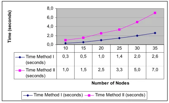
Figure 16. Time Versus Number of Nodes for both Method I and II ... 44

Figure 17. Time Versus Number of Swimlanes for both Method I and II ... 45

Figure 18. (a) Activity Diagram I (b) Layout by Method I (c) Layout by Method II ... 52

Figure 19. (a) Activity Diagram II (b) Layout by Method I (c) Layout by Method II... 53

Figure 20. (a) Activity Diagram III (b) Layout by Method I (c) Layout by Method II ... 54

Figure 21. (a) Activity Diagram IV (b) Layout by Method I (c) Layout by Method II ... 55

Figure 22. (a) Activity Diagram V (b) Layout by Method I (c) Layout by Method II ... 56

Figure 23. (a) Activity Diagram VI (b) Layout by Method I (c) Layout by Method II ... 57

(9)

1

Chapter 1 Introduction

1

1 .

.

1

1 O

O

v

e

r

v

i

e

w

The Unified Modeling Language (UML) is a language and notation for specification, construction, visualization, and documentation of models of software systems. In other words, UML is a graphical language derived from several existing notations commonly used to specify the design of object-oriented software. Since UML takes the increased demands on today’s systems into account, and covers a broad spectrum of application domains, it has become the standard for specifying aspects of object-oriented software systems in the last few years [30].

Graph drawing has become an important area of research in Computer Science for the last couple of decades. There is a wide range of applications related to this area including data structures, databases, software engineering, VLSI technology, electrical engineering, production planning, chemistry, and biology. Graph layout diagrams are a common way of writing down and communicating ideas. With graph layout techniques, the readability and the comprehensibility of the graphs increases and the complexity is reduced. As a result of this, we use them for all sorts of things including UML diagrams. In this thesis, we present new graph layout algorithms for drawing UML activity diagrams using constrained hierarchical layout implemented by Tom Sawyer Software.

A UML diagram contains visual elements that represent model elements coming from different packages, even in the absence of visibility relationships between these packages. The diagrams may show all or parts of the characteristics of the model elements, with a level of detail that is suitable in the context of a given diagram. Diagrams may also gather

(10)

class [29].

Here, in alphabetical order, is a list of the various diagrams:

· Activity diagrams represent the behavior of an operation as a set of actions and will be explained in detail in the next section.

· Class diagrams represent the static structure in terms of classes and relationships.

The class diagram provides a static structure of all the classes that exist within the system. They show the various classes, each defined through a set of attributes and methods, and points out the relationship between each of those classes via associations, inheritance, etc. and also includes an indication of their cardinalities, but without any temporal information. Figure 1 analyses the class diagram of Contact Point system. Surface Address, Phone Number, Business Entity are some of the classes, while the lines joining the different classes refer to their relationship [29].

(11)

· Collaboration diagrams are a spatial representation of objects, links, and interactions. They focus upon the relationships between the objects. They are useful for visualizing the way several objects collaborate to get a job done and for comparing a dynamic model with a static model. Collaboration and sequence diagrams show the same information, and can be transformed into one another without difficulty.

· Component diagrams represent the physical components of an application.

These diagrams focus on the responsibilities of the objects and their structural organization. In addition, they show a set of interactions between distinguished objects in a limited context. They are semantically equivalent to sequence diagrams. For the disadvantages of these diagrams, we can include the followings: missing time axis, and missing source of invocation [31].

· Deployment diagrams represent the deployment of components on particular pieces of hardware.

· Object diagrams represent objects and their relationships and correspond to simplified collaboration diagrams that do not represent message broadcasts.

· Sequence diagrams are a temporal representation of objects and their interactions.

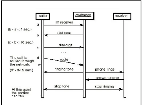
A sequence diagram shows the objects participating in the interaction and the messages that they exchange arranged in time sequence. In these diagrams, objects are represented as vertical lines and messages as horizontal lines. They are useful in systems that have time-dependent functions, for example, in real-time applications or in those systems where time dependencies play an important role. These types of UML diagrams represent the chronology of message passing more efficient. They are semantically equivalent to Collaboration diagrams. Its great strength comes from its simplicity. The principal weakness of collaboration diagrams is that they describe behavior but they do not define it [29, 31].

(12)

Figure 2: A Sequence Diagram

Figure 2 is a model of a telephone system using sequence diagram. The three objects present are the caller, the exchange and the receiver. The following can be deduced from the diagram. Firstly, the caller sends a message of type ‘lift receiver’ to the exchange. Only then does the exchange send back a message of type ‘dial tone’ to the caller. The sequence of interaction reads down the page [32].

· Statechart diagramsrepresent the behavior of a class in terms of states

Behavior of a system often depends on an internal state. Statecharts visualize the sequence of states of an object or interaction during its lifetime. They are useful for describing behavior of an object in several use-cases. While using statechart diagrams, one has to define all the possible states of a system. There is one problem encountered here, there can be exponential growth in the number of states. However, separating state-transition diagrams for each class

(13)

can prevent this. These diagrams are very powerful but its semantics is not very clear. This problem can also be solved by introducing constraints to restrict the semantics [29, 31].

Figure 3: A Statechart Diagram

Figure 3 is an example of a statechart diagram for a bank account. The rectangles represent the various states that the account can be in and the arrows correspond to the transitions due to the call of a method on the object.

· Use case diagrams represent the functions of a system from the user's point of view. The Use Case diagram consists of two main components, the Actors and the Use Cases. An Actor is any person, organization or computer system, external to the system, but interacting with it. The Use Cases are the interfaces that the system makes visible and available to the outside world through which the latter can interact. Actors are illustrated as stick figures; use cases as ovals and the system as a box. The diagram is therefore appropriate for illustrating the software from a user's perspective. This is because it provides an external view of the system, without defining the actual internal structure of the system [30].

A simple university information system could make use of the following use cases: enroll students in courses, input student course marks, and produce student transcripts. Figure 4 illustrates the above example. The actors are the students, the lecturer and the registrar.

(14)

Figure 4: A Use Case Diagram

Sequence and collaboration diagrams can be grouped together under the more general title of interaction diagrams.

First of all, we will try to explain some major points about UML then we will focus on especially activity diagrams.

1

1 .

.

2

2 U

U

M

L

M

e

t

a

-

M

o

d

e

l

UML is unique in that it has a standard data representation. This representation is called the meta-model. The meta-model is a description of UML in UML. It describes the objects, attributes, and relationships necessary to represent the concepts of UML within a software application.

(15)

1

1 .

.

3

3 T

T

h

e

N

o

t

a

t

i

o

n

o

f

U

M

L

The UML notation is rich full bodied. It is comprised of two major subdivisions. There is a notation for modeling the static elements of a design such as classes, attributes, and relationships. There is also a notation for modeling the dynamic elements of a design such as objects, messages, and finite state machines. Static models are presented in diagrams including class diagrams while activity diagrams can be given as an example of dynamic structures of UML.

1

1 .

.

4

4 A

A

c

t

i

v

i

t

y

D

i

a

g

r

a

m

s

The OMG Unified Modeling Language Specification defines an activity diagram as: "…A variation of a state machine in which the states represent the performance of actions or sub activities and the transitions are triggered by the completion of the actions or sub activities. It represents a state machine of a procedure itself." [29]

When we design our operation specifications, we are describing what the operation will do. When we get to implementation, we have to decide how the operation will do what we specified. For many operations, this is very easy because the operations are not overly complex. For more complex operations, however, it is not so easy, which is where operation architectures using activity diagrams are useful. An activity diagram is a special form of state diagram used to model a sequence of actions and conditions taken within a process.

The purpose of the activity diagram is to model a workflow process and/or to model operations. Activity diagrams tell us the procedural possibilities of a system with the aid of activities.

1

1 .

.

4

4 .

.

1

1 D

D

e

f

i

n

i

t

i

o

n

s

a

n

d

N

o

t

a

t

i

o

n

An activity is a single step in a processing procedure. It is a state with an internal action and at least one outgoing transition. The outgoing transition implies termination of the internal action. An activity can have several outgoing transitions if these can be identified through conditions.

(16)

Activity diagrams are similar to procedural flow charts, except that all activities are uniquely associated to objects. They support the description of parallel activities. For activity paths running in parallel, the order is irrelevant. They can run consecutively, simultaneously, or alternately.

1

1..44..11..11IInniittiiaallaannddFFiinnaallSSttaatteess

A filled circle followed by an arrow represents the initial action state. An arrow pointing to a filled circle nested inside another circle represents the final action state. Figure 5 shows an initial and end state notation used in activity diagrams.

a) Initial State b) Final State

Figure 5: Initial and Final States

1

1..44..11..22AAccttiivviittyyaannddTTrraannssiittiioonn

The essential symbol of the activity diagram is the activity. It is represented by a straight line at the top and bottom, enclosed by an arc on each end. An activity is a major task that must take place in order to fulfill the operation contract. The activity description, which can be a name, a freely formulated description, a pseudo-code or a programming language code, is placed in the symbol.

Incoming transitions trigger an activity. If several incoming transitions exist for an activity, each of the transitions can trigger the activity independently from the others. Each activity has one or more arrows emerging from it. The arrows represent the transition between one activity and the next. Outgoing transitions are drawn in the same way as event arrows, but without an explicit

(17)

event description. Transitions are triggered implicitly by the termination of the activity. Figure 6 shows two activities. When activity 1 terminates, it triggers the transition 1. Then transition 1 triggers activity 2.

Transition1

Figure 6: A Simple Activity Diagram

1

1..44..11..33BBrraanncchhiinnggaannddDDeecciissiioonnss

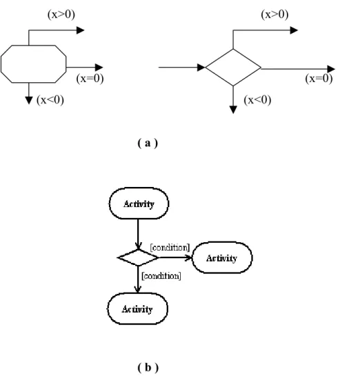
Outgoing transitions can be provided with conditions enclosed in square brackets. Such conditions should be Boolean expressions; branching points may be used. Instead of binding the conditions directly to the transitions leaving the activity, for convenience a stereotype is provided for a decision: the traditional diamond shape, with one or more incoming arrows and with two or more outgoing arrows, each labeled by a distinct guard condition with no event trigger. This diamond too represents a decisional activity. Figure 7 show an example of conditions in activity diagrams. A decision may be shown by labeling multiple output transitions of an action with different guard conditions.

(18)

(x>0) (x>0) (x=0) (x=0) (x<0) (x<0) ( a ) ( b )

Figure 7: (a) Condition Figures (b) Activity Diagram with a Condition

1

1..44..11..44SSyynncchhrroonniizzaattiioonnaannddSSpplliittttiinngg

Moreover, transitions may be synchronized and split. These situations are represented by short thick lines into which transitions bump or from which they leave. Figure 8 shows

synchronization and splitting. When there are concurrent event(s) triggering an activity or

activities then a horizontal synchronization bar is drawn between event and activity. A short heavy bar with two transitions leaving it represents a splitting of control that creates multiple states.

(19)

Synchronization Splitting

( a )

( b )

Figure 8: (a) Synchronization and Splitting (b) An Example

1

1..44..11..55OObbjjeeccttSSttaattee

Activities cause changes in object states. Object states are represented as rectangles that contain the name of the object and, enclosed in square brackets, the object state. Activities and object states are joined by dashed transition lines. If the line leads from an object state to an activity, this means that the activity presumes or requires an initial state. If the line leads from an activity to an object state, this shows the state resulting from the activity. Figure 9 shows an example of a change in an object state as a result of activity1.

(20)

Figure 9: Change in Object State

1

1..44..11..66SSwwiimmllaanneess

Activity diagrams can be subdivided into responsibility domains, the so-called swimlanes, which allow activities to be assigned to other elements or structures. For example, the class or component the activities belong to can be stated. If activity diagrams are employed for analysis and business process modeling, swimlanes can also be used to map organizational structures.

Swimlanes often correspond to organizational units in a business model. An activity diagram may

be divided visually into ''swimlanes'' each separated from neighboring swimlanes by vertical solid lines on both sides. Each swimlane represents responsibility for part of the overall activity. Transitions may cross lanes; there is no significance to the routing of a transition path.

Swimlanes enable you to partition activities into groups based on responsibility for carrying out the activities. You could have swimlanes for different objects when modeling operation workflow, or different business entities when modeling business process workflow. For example, in an airline reservation context, you might have separate swimlanes for Customer and Ticket Agent. As it can be seen in Figure 10, taking and delivering order activities are the responsibilities of the sales department of a firm while filling order activity is the responsibility of the distribution department. Therefore, these two responsibilities are divided by a swimlane.

Object

(21)

( a )

( b )

Figure 10: (a) Swimlane Prototype (b) A Practical Example with Swimlanes

1

1 .

.

4

4 .

.

2

2 A

A

n

O

v

e

r

a

l

A

c

t

i

v

i

t

y

D

i

a

g

r

a

m

E

x

a

m

p

l

e

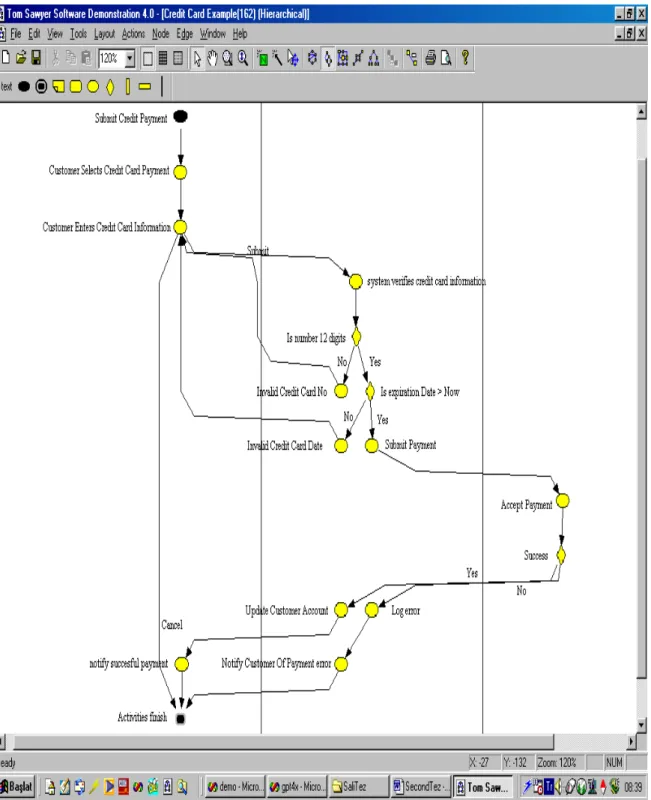
The example in Figure 11 is a credit card payment submission. The activity diagram begins with a Presentation to the customer that specifies the credit card payment; the customer then enters and submits his/her card details. The system validates these values and either returns to the customer if there is an error or submits the payment to the Credit Card Service. If the card payment is accepted, then the system notifies the customer of success. If not, then the error is logged, and the customer is notified of the failure (and perhaps directed to handle the payment

(22)

Service is unavailable, and also additional system accounting activities.

Figure 11: An Overall Activity Diagram

1

1 .

.

4

4 .

.

3

3 A

A

d

v

a

n

t

a

g

e

s

&

D

i

s

a

d

v

a

n

t

a

g

e

s

o

f

U

s

i

n

g

A

c

t

i

v

i

t

y

D

i

a

g

r

a

m

s

In systems development, design is usually the first thing to go when schedules are tight. The lack of design leads to non-maintainable, non-reusable systems, full of spaghetti code and repeated functionality. Some of the problems inherent in the waterfall development process are alleviated

(23)

by adopting an object-oriented, iterative, short-cycle small-deliverable approach to systems delivery. More relief may be found in the fact that many of the operations specified during analysis will be so simple that no real design effort is required. Cycle time is reduced even more if your organization has established a reuse process. Even if all of these factors are in your favor, the fact remains that there will always be those big monster operations that should not be tackled without a good design. The first step to a good design for these monster operations is the activity diagram [33].

Activity diagrams are useful behavioral modeling tools for the following reasons: · They describe the internal behavior of an operation pictorially

· They depict activities that can occur in parallel

· They help to identify activities whose responsibility belongs elsewhere · They allow the discovery of common functionality within a system · They can be used as coding specifications

The activity diagram focuses on activities, in this sense it is like a flow chart supporting compound decisions. However, it differs from a flow chart by explicitly supporting parallel activities and their synchronization. In other words, we want to look for activities that can occur in parallel. Many of us have become accustomed to describing processes sequentially. The discovery of activities that can occur in parallel will help us to build processes that are more efficient.

The biggest disadvantage of activity diagrams is that they do not make explicit which objects execute which activities, and the way that the messaging works between them. Labeling of each activity with the responsible object can be done. Often it is useful to draw an activity diagram early on in the modeling of a process, to help you understand the overall process. Then interaction diagrams can be used to help you allocate activities to classes.

(24)

16

Chapter 2 Related Work

The related work in our thesis can be summarized under three topics: Graph Layout, and Types of Graph Layout and Constrained Graph Layout. Firstly, we give general information about graph layout. Since we especially use Tom Sawyer Software’s implementation of constrained hierarchical layout to layout UML activity diagrams in this thesis, we emphasize hierarchical layout, Sugiyama Algorithm and constrained graph layout in this chapter.

2

2 .

.

1

1 G

G

r

a

p

h

L

a

y

o

u

t

Graphs, consisting of a set of nodes and a set of edges, are one of the most fundamental ways of representing relationships among objects. Programs that display a set of relationships as a graph have become more prevalent in recent years because of the following reason. That is, a person is usually able to comprehend information better when it is presented pictorially rather than in textual form. This is partly due to the fact that structural properties such as planarity, symmetry, and hierarchy are readily apparent from a well-drawn graph and recognition of these properties seems to help the user understand the graph [2].

It is known that a number of data presentation problems involve the drawing of a graph on a two-dimensional surface. Examples include circuit schematics, algorithm animation, and software engineering. Within a graphic standard, a graph has infinitely many different drawings. However, in almost all data presentation applications, the usefulness of a drawing of a graph depends on its readability, that is, the capability of conveying the meaning of the diagram quickly and clearly.

Readability issues are expressed by means of

aesthetics, which can be formulated as optimization goals for the drawing algorithms. In general,

(25)

interest. A fundamental and classical aesthetic is the minimization of crossings between edges. Among other aesthetics are displaying symmetries, avoiding bends in edges, keeping edge lengths uniform, and distributing vertices uniformly [1, 2, 7].

2

2 .

.

2

2 T

T

y

p

e

s

o

f

G

r

a

p

h

L

a

y

o

u

t

We can classify graph layout into two branches: According to aesthetic views of them and the underlying algorithms, which they are based on.

2

2 .

.

2

2 .

.

1

1 A

A

c

o

r

d

i

n

g

t

o

A

e

s

t

h

e

t

i

c

V

i

e

w

s

2

2..22..11..11CCiirrccuullaarrLLaayyoouutt

The circular layout algorithm divides the nodes of an input graph into clusters. These clusters are based on either the natural group structure inherent in the topology of the graph or upon certain application specific data (e.g., IP addresses). The graph of such clusters, known as a cluster

graph, will be formed of a relatively highly connected subgraph and a list of trees. The subgraph

will consist of main site clusters, while the tree lists will consist of peripheral or subsite clusters.

The circular representation of graphs has direct applications in network and systems management, knowledge representation, WWW visualization, social networking, and criminology.

Main site clusters are placed around a virtual cluster. The order of main site clusters and the order of nodes within each main site cluster are optimized with the help of heuristics to minimize edge crossings.

(26)

2

2..22..11..22OOrrtthhooggoonnaallLLaayyoouutt

Orthogonal layout emphasizes clear and organized structures of a graph. In particular, this is done by placing nodes onto a grid of rows and columns and by routing edges to run parallel to (x, y) axes in orthogonal drawings. A grid consists of columns that are parallel to the y-axis and rows that are parallel to the x-axis. Nodes are placed at different positions in rows and columns. A node may occupy several rows and columns depending on the node height and width. In addition, a node is forced to span extra rows and columns if it has more than one incident edge on any one side [4].

Edges are visually represented by line segments that run along rows and columns. The route of each edge traverses a series of intersecting rows and columns in the grid. Normally each edge is drawn with at most one bend.

The applications well suited to the use of the orthogonal layout are physical and logical database design applications, software reengineering applications, CAD diagrams, and OOA/OOD diagrams.

2

2..22..11..33SSyymmmmeettrriiccLLaayyoouutt

Symmetric layout algorithm uses heuristic for computing best symmetric graph layout. Heuristic picks the node that is farthest out of place, and iteratively moves it closer to its ideal position. Algorithm assumes that all nodes have repulsive and attraction forces. The task is to find the graph layout in which these forces are stable/balanced. Good layout is considered when the energy is low [4].

The symmetric layout is useful in a number of application domains. These include wide-area networks, enterprise networking, database schemata, systems management, knowledge representation, and WWW visualization.

(27)

2

2..22..11..44TTrreeeeLLaayyoouutt

The tree layout algorithm first calculates the optimal spanning tree for the given graph. The edges of the graph will consist of tree edges, which form the skeleton of the drawing, and non-tree

edges, or all other edges of the drawing.

Each tree has a distinguished node called its root. The root node is the source of a tree and it is the only node without a parent. Every node in a tree has one or more children connected to it. The connections between parent and child nodes are called tree edges. Tree edges are always routed as short, straight lines. Non-tree edges, by contrast, often span multiple tree levels and are routed over a sequence of bend points [4, 8].

In order to emphasize a tree structure, the nodes are organized into levels and are repositioned based upon the tree edges alone. A tree level is formed by a group of nodes placed along a horizontal line. The root node is always placed at the top-most level. A parent node is placed to be centered one level above its children; all siblings are placed at the same level. Each tree edge connecting a parent node to its child is said to be a tree branch [4].

Applications using tree layout include social network applications, process modeling tools, project management software, UML diagrams, and software development tools.

2

2..22..11..55HHiieerraarrcchhiiccaallLLaayyoouutt

The hierarchical layout style shows precedence relationships and is commonly used to represent organizational dependencies, process models, software call graphs, networks, and information management systems.

For the hierarchical style, a graph can be oriented four different ways: top-to-bottom, bottom-to-top, right-to-left, and left-to-right. As an example, when a graph is oriented top-to-bottom, the source nodes are positioned near the top of the page, and the target nodes are positioned near the bottom [1, 4].

(28)

For the hierarchical style, a proper hierarchical layout of a graph is created by default. In a proper hierarchy, the nodes of a directed graph are partitioned into groups called levels. Each node in a level shares a common y coordinate if the levels are oriented horizontally, and a common x coordinate if the levels are oriented vertically. Each edge in the graph connects two nodes that belong to different levels. If an edge spans more than one level, it is decomposed into a series of segments, each segment spanning a single level [1].

2

2 .

.

2

2 .

.

2

2 A

A

c

o

r

d

i

n

g

t

o

U

n

d

e

r

l

y

i

n

g

A

l

g

o

r

i

t

h

m

s

There are many algorithms produced for drawing graphs aesthetically. We will generally explain these algorithms but especially we will emphasize on Sugiyama Algorithm since the newly created algorithms in the thesis were prepared by using constrained hierarchical algorithm based on Sugiyama.

2

2..22..22..11FFoorrccee––DDiirreecctteeddLLaayyoouuttAAllggoorriitthhmmss

There are mainly two different force-directed graph layout algorithms that are Spring-Embedder and Local Temperatures methods.

For Spring-Embedder type algorithms such as Kamada and Kawai’s algorithm, and A. Frick and A. Ludwig’s algorithm use an analogy to physics. Vertices are treated as mutually repulsive charges and edges as springs connecting and attracting these charges. Starting with an arbitrary initial placement of vertices, the algorithm iterates the system in discrete time steps by computing the forces between vertices and updating their position accordingly. The algorithm stops after a fixed number of times [11].

The algorithms using local temperature are based on the attraction of vertices towards their barycenter and the detection of oscillations and rotations. For each vertex, a local temperature is defined that depends on its old temperature and the likelihood that the vertex oscillates or is part of a rotating subgraph. Local temperatures rise if the algorithm determines that a vertex is

(29)

probably not close to its final destination. The global temperature is defined as the average of the local temperatures over all vertices. Thus, it indicates how stable the drawing of the graph is [7].

2

2..22..22..22IInnccrreemmeennttaallLLaayyoouuttAAllggoorriitthhmmss

In most applications, it is helpful to preserve an overall “mental map” of the drawing of a changing graph. Incremental layout maintains the relative positioning information from a graph’s previous layout. This yields a more “stable” drawing that preserves its overall form despite minor modifications to the graph in the course of successive layouts [7].

Because the algorithms for incremental layout work from an existing layout, they often run faster than algorithms that must produce a layout starting from scratch.

2

2..22..22..33SSuuggiiyyaammaaBBaasseeddAAllggoorriitthhmmss

Sugiyama [1] describes the method to compute a visualization of hierarchical system structures by applying the following algorithm, which consists of four steps:

Step 1. Partitioning of nodes and edges There are mainly two parts under step 1:

a. Rank assignment of vertices:

This phase of Sugiyama algorithm partitions the visible nodes into levels. An integer rank is calculated for each node. All nodes with the same rank form a level and are laid on the same vertical position. The ranks correspond to the depth of the nodes in a spanning tree of the graph [1].

There are many possibilities to calculate the rank:

· Calculate a spanning tree by depth first search or breath first search. This has the time complexity with orderúVú+úEú, but it results an arbitrary partition.

(30)

where C is the cost function on edges. Because the edges of the spanning tree are later drawn between adjacent levels, these edges are rather short. The complexity of this algorithm is O(çEçlogçVç).

· If the graph is acyclic, then we can use topological sorting to calculate the rank. In this method, we can assign nodes to levels according to their depth (longest path of predecessors) in the graph. Cycles in the graph are handled by temporarily reversing the direction of an edge. The rank of any vertices (R(v) as a function) is set to max{R(w)çw is predecessor of v}+1. This algorithm needs time O(çVç+çEç).

b. Transformation of the original graph into a proper hierarchy: First of all, we should define the proper hierarchy of a graph.

An n-level hierarchy (n>=2) is defined as a directed graph (V, E), where V is called a set of vertices and E a set of edges, which satisfies the following conditions.

1. V is partitioned into n subsets, that is

V = V1È V2È... Vn (ViÇ Vj = Æ, i ¹ j) where Vi is called the ith level and n the length

of the hierarchy.

2. Every edge e= (vi , vj) Î E, where viÎ Vi and vjÎ Vj, satisfies i<j, and each edge in E is

unique.

The n-level hierarchy is denoted by G = (V, E, n). An n-level hierarchy is called “proper” when it satisfies further the following conditions:

3. E is partitioned into n-1 subsets, that is E = E1È E2È... En-1 (EiÇ Ej =Æ, i ¹ j),

where EiÌ Vi X Vi+1, i =1,2,...n-1.

4. An order si of Vi is given for each i, where the term “order” means a sequence of all

vertices of Vi ; si = v1 v2... vçViç (çViç denotes the number of vertices of Vi). The n-level

(31)

To construct a proper hierarchy from G = (V, E), upward edges are reversed. Of course, they are marked such that arrowheads in the drawing will show the original direction. Furthermore, edges crossing several levels (long span edges) are split into small edges and dummy nodes [1].

Step 2. Reduction of number of crossings

The hierarchy calculated in step 1 often contains many edge crossings that should be eliminated in this step. The order of the nodes within a level determines the edge crossings in the layout, and a good ordering is one with few crossings. The problem of minimization of edge crossings in layouts of ranked graphs is NP-complete, even for only two ranks. There are some heuristics for finding the ordering of vertices with minimum edge crossing including Barycentric method (BC

method) [1, 19].

In Barycentric method where the goal is to reduce the crossings with the adjacent level, the relative positions of nodes within each level are determined. Each node is positioned based on its

barycenter that, roughly speaking, is the average position of its predecessors (or successors).

Several upward and downward passes are made through the graph until no improvement is detected or a threshold value has been reached.

There are two phases in reducing the number of crossings: calculation of crossings, and

reordering of nodes.

Step 3. Improvement of horizontal positions of vertices (Fine-tuning)

The actual (x, y) coordinates of each node are determined. The fine-tuning shifts nodes within their level to center nodes in respect to their predecessors or successors. The relative position of the nodes is not allowed to change, so this phase will not contribute to any more (or less) edge crossings. The Pendulum method or the Rubber band method can be given as examples of the finetuning algorithms. The aesthetic criterion “symmetry”, which requires that a node v be placed in the middle of all adjacent nodes with edges to v, is the main aim for these methods [1, 2].

(32)

A two-dimensional picture of the hierarchy is automatically drawn where the dummy vertices and edges are deleted and the corresponding long span edges are regenerated.

2

2 .

.

3

3 C

C

o

n

s

t

r

a

i

n

e

d

G

r

a

p

h

L

a

y

o

u

t

Graph layout can either be done manually meaning that each node and edge is placed by the user or automatically, meaning that an algorithm computes the position of the nodes and edges to produce an aesthetic drawing.

Automatic layout has the advantage of relieving the user of the tedious chore of the layout. However, it usually does not produce quite as good results as a manual layout. One of the main reasons is that most automatic layout algorithms are not designed to take a user’s layout

constraints into account. For example, the user might request that one node to be left of another

or that a particular group of nodes be placed near each other. Since these constraints are specified explicitly, they are of higher priority than the aesthetic goals of the layout algorithm [2].

In this section, we present the management of constrained layout used in Tom Sawyer Software’s implementation. First of all, we define the infrastructure of this system including low level constraints and how they can be added to the layout system, and then give information about the constraint managers. Afterwards, we explain how the constraints added to the system are managed and taken into account when hierarchical layout is performed. Specifically, we investigate the integration of constraint management system with hierarchical layout algorithm as implemented by Tom Sawyer Software in its Graph Editor Toolkit (GET)1.

(33)

2.3.1 Infrastructure of Constrained Graph Layout

The infrastructure of constrained GL system used in GET is divided into three parts: low level constraints, the constraint manager, and consistent constraint graphs produced.

2

2..33..11..11LLoowwLLeevveellCCoonnssttrraaiinnttss

First let us describe the kind of constraints that a user would like to have. To constrain the position of a node in a graph, there might be three different types of constraints [2]:

· Absolute Positioning: It constrains the node’s position in regards to a fixed coordinate system. For example, assuming that nodes are placed in horizontal levels, placement of a node to a particular level can be a constraint.

· Relative Positioning: It constrains the node’s position in relation to other nodes. For example, it can be given as node A is left of node B or as node C is the top neighbor of node D.

· Clusters: It gathers a group of nodes together to a cluster. For example, all nodes in cluster F are to the right of node G.

In GET’s constrained graph layout management system, these low level constraints are realized by the following constraint types: order constraints and level constraints.

There are six different kinds of order constraints implemented by the methods summarized below [28].

· AddHOrderConstraintOneNode: This method creates an order constraint for the input node. It creates an order constraint which can force the node to be the left most, right most (if levels are horizontal) or the top most, the bottom most (if level are vertical) node in its level.

(34)

nodes. This constraint will force the nodes given as a list to be placed from left to right in the order how they show up in the list.

· AddHOrderConstraintTopOfChain: This method creates an order constraint for each of the input nodes. It will force the nodes given as a list to be placed from top to bottom in the order how they show up in the list.

· AddHOrderConstraintLeftOfSets: This method creates order constraints for the input nodes. It will force the nodes in the first list to be placed left of the nodes in the second list, regardless of whether all nodes are in the same level or not. This is the only constraint that controls the relative horizontal position of nodes in different levels.

· AddHOrderConstraintTopOfSets: This method creates order constraints for the input nodes. It will force the nodes in the first list to be placed top of the nodes in the second list, regardless of whether all nodes are in the same level or not. This is the only constraint that controls the relative vertical position of nodes in different levels.

· AddHOrderConstraintStraightEdges: This method creates a constraint for each end node of the edges in the input list. The new constraint will force the edges in the list to be straight lines.

There are three different kinds of level constraints implemented by the methods summarized below [28].

· AddHLevelConstraintOneNode: This method creates a level constraint for the input node. It creates a level constraint which can force the node to be ending up in a level with a level number at least a given level, or at most a given level. Or it can be placed in a level with the given level number. In addition, the node also can be end up in a level with the highest possible level.

· AddHLevelConstraintHigher: This method creates a level constraint for the input nodes. The new constraint will force the nodes in the first list to end up in a level with a number at least a given number (distance) higher than the number of the level where the nodes in the second list will end up.

(35)

· AddHLevelConstraintLevelRange: This method creates a constraint for each of the nodes in the input list. The new constraint will force the nodes in the list to end up in a bundle of level that are close together: The number of the level with the largest number minus the number of the level with the smallest number has to be smaller than 'range'. A range value of 1 means than all nodes share a same level.

As you can see, different dimensions are treated independently from each other. In other words, level constraints represent constraints related to the y coordinates while order constraints represent constraints related to x coordinates.

2

2..33..11..22TThheeCCoonnssttrraaiinnttMMaannaaggeerr

For each dimension (x and y or level and order), there is a constraint manager which has two main tasks. The first is that it maintains a list of all constraints and provides functionality to add, delete, and query the status of constraints in the constraint graph. The other is that it evaluates the constraint graph and makes sure it is consistent. A set of constraints is defined to be consistent if none of them are contradictory [2, 23, 24].

The purpose of the evaluation of the constraint graph is to compute the global effects of local constraints. This evaluation can be done in linear time in the number of the constraints by an algorithm based on topological sorting. By doing so, extensive computations can be avoided while reordering the nodes [2, 25, 26].

If there are contradictory constraints, the constraint manager computes a subset of consistent constraints by eliminating some of the constraints. This elimination process could be done by giving low priorities to deactivated constraints. The constraint manager then tries to keep high priority constraints active, while some low priority constraints are deactivated. Deactivated constraints are ignored during the evaluation of constraint graphs [27].

(36)

Layout

As we stated before, the main work done in Sugiyama Algorithm is reduction of number of crossings phase. During this phase, a total ordering of the nodes in each level is determined. After computing the ordering of the nodes, corresponding constraints are given to the constraint manager. They receive a low priority so that in determining the final ordering, the constraint manager will give preference to user or application specific constraints. Here the important thing is that the constraint managers should be efficient since there might be a large number of constraints and the levels are rearranged frequently.

(37)

29

Chapter 3 Proposed Methods

As stated before, our aim was to produce a new hierarchical layout technique to layout UML activity diagrams using Tom Sawyer Software’s implementation of constrained hierarchical layout. For reaching this goal, we have customized Tom Sawyer Software’s GET to create and edit UML activity diagrams. Thus, we have started by adding a toolbar called Activity Diagram Tool Bar to GET. This toolbar included necessary types of objects and links that a UML activity diagram contains.

After this step, assuming that the activity diagram objects except swimlanes are ordinary node-like objects, there was only one problem left to be solved, implementation of swimlanes. We have achieved this by implementing a new type of diagram object to separate swimlanes, which stores its x value2 and can be created, deleted, and moved just like other objects.

Finally, we needed to customize GET for the layout of activity diagrams. This extension of GET handles the hierarchical layout of activity diagrams with swimlanes. The basic rule is that, each node belonging to a swimlane (namely, nodes drawn immediately to the left of a swimlane separator) should remain to be immediately to the left of the same swimlane separator after applying the layout algorithm. For this crucial step, we have developed two different methods. While developing these methods, we have used GET’s constrained addition methods described earlier.

For these two methods, we have three steps in general. These are 1. Pre-processing Step

(38)

implementation)

§ Level Assignment

§ Crossing Reduction and Solving Constraints § Fine-tuning

3. Post-processing Step

Each of the two methods is applied in the pre and post-processing steps, not directly interfering with the hierarchical layout step.

In the remaining of this chapter, we first explain the methods mentioned. Then a short technical analysis of the methods will be provided. Afterwards, performance evaluation of the methods is presented.

3

3 .

.

1

1 M

M

e

t

h

o

d

I

During the pre-processing step, we first determine the swimlanes to which each node belongs. In other words, we identify the swimlane separator for node n whose x position is equal or bigger than node n’s x position but is the smallest among all the swimlanes. The rightmost nodes that are not to the left of any swimlane separator are given null swimlane values.

In this step, we give constraints to the layout system as follows. For each swimlane, we determine two lists of nodes. The first node list is composed of the nodes belonging to this swimlane, and the other one is formed of all the remaining nodes. Then we give these two node lists to the constraint creation system. The new constraint will force the nodes in the first list to be placed to the left of the nodes in the second list, regardless of whether all nodes are in the same level or not. This is the only constraint that controls the relative horizontal positions of nodes in different levels. The parameter 'priority' allows the user to specify which constraint will be respected in the case of conflicting constraints (the lower priority wins).

After completing constraint additions, constrained hierarchical graph layout starts. This step is the same as Sugiyama algorithm explained before, except that the constraints are taken into

(39)

account in the crossing minimization step. The constraints generated during constraint addition are taken into consideration while reordering the nodes for each level.

The next phase, namely the post-processing step, involves determining the new positions of the swimlanes and nodes, and moving them to these new coordinates. First of all, we try to find a swimlane separator’s new position in such a way that among nodes belonging to the associated swimlane, the rightmost node is found and then the new x position of the swimlane separator is equal to the right side of the node’s rectangle’s x position plus a predetermined number of units. However, we also push all the nodes that come after the swimlane separator by the predetermined number of units. For each swimlane, this process is repeated, and the final positions of the nodes and swimlanes are determined at the end.

3

3 .

.

2

2 M

M

e

t

h

o

d

I

In the pre-processing step, there are two sub steps for this method. First we determine the swimlanes to which each node belongs as in Method I. However, different from Method I, we create a dummy node for each swimlane separator as a representative and we adjust its x coordinate to be the same as the separator. Thus, we can think of the diagram as if there was no swimlanes. During constraint addition sub step, we give constraints to the system as follows. For each dummy node, we provide two constraints: the first constraint is that the nodes that belong to the swimlane that is immediately to the left of the swimlane separator corresponding to each dummy node must be again to the left of this dummy node after layout. Similarly the nodes that belong to the right neighboring swimlane should stay to the right of this dummy node after lay out.

After completing the constraint addition step, constrained hierarchical graph layout step starts and works as explained in Method I.

The next phase, namely post-processing step, involves determination of the new positions of the swimlane separators by simply assigning them the x coordinate of the corresponding dummy node. After that we delete these temporary dummy nodes from the graph.

(40)

3

3 .

.

3

3 T

T

e

c

h

n

i

c

a

l

A

n

a

l

y

s

i

s

o

f

t

h

e

M

e

t

h

o

d

s

3

3 .

.

3

3 .

.

1

1 P

P

e

r

f

o

r

m

a

n

c

e

E

v

a

l

u

a

t

i

o

n

There are generally three major points to be explored while evaluating the methods developed. They are summarized as aesthetic views of the layouts of corresponding methods, and time and space complexities.

3

3..33..11..11AAeesstthheettiiccVViieewwCCoommppaarriissoonn

We can compare the aesthetic view of layouts obtained from both methods with the original activity diagram by means of giving different layout examples and this should give a general idea of how these two methods perform with respect to aesthetic view as well as an opportunity to contrast the two.

(41)

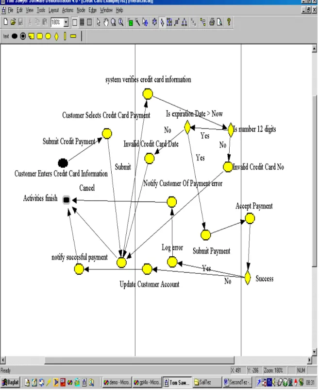
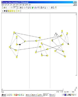
Figure 12: The Activity Diagram of Figure 11 drawn using Our Activity Diagram Editor developed using GET. The diagram is laid out pretty much randomly, respecting swimlanes.

(42)

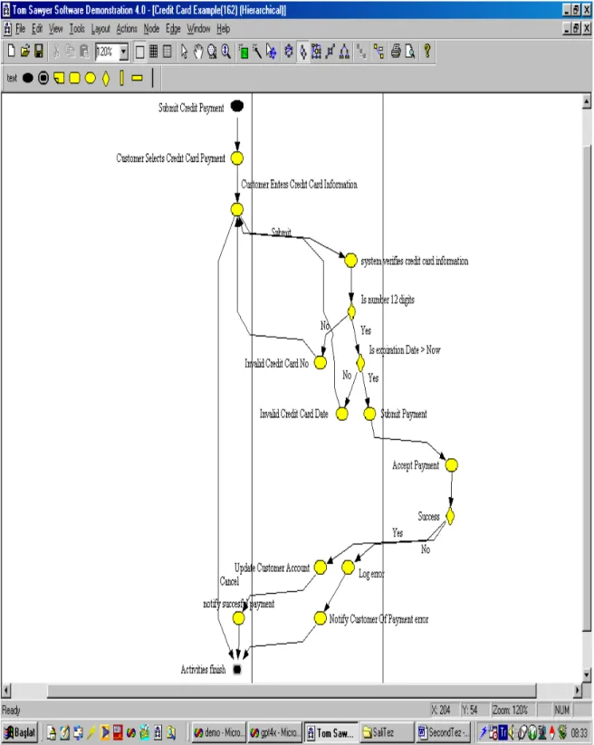
Figure 13: The Hierarchical Layout of Figure 12 Using Method I

(43)

Figure 14: The Hierarchical Layout of Figure 12 Using Method II

As can be seen in Figure 12, we have drawn the activity diagram of Figure 11 using our activity diagram editor developed on top of GET. Then, we have laid out this activity diagram by using our methods (Figures 13 and 14 give the results obtained, respectively).

(44)

When we compare the layout results, we can certainly say that our methods for drawing UML activity diagrams hierarchically give better aesthetic results. For example, the layouts we generated are more uniform, and they have less number of edge crossings. Moreover, they are more readable and comprehensible than the diagram before layout. Therefore, we can safely say that the layout is worthwhile.

When contrasted Method I gives a narrower layout than Method II. Therefore this makes the activity diagram more complex than the one produced by method II. In other words, method II makes use of area more fairly than the method I. However, the situation that Method I gives a narrower layout is directly related to the space left between the nearest node to a swimlane separator during Method I. If we increase this space then we can make the layout less complex.

Another major difference between these two layouts is the way the edges are laid out. Namely, in Method I edges have somewhat unnecessary bend points such as on the edge from the activity “Invalid Credit Card Date” to the activity “Customer Enters Credit Card Information”. However, in Method II, edges do not have these unnecessary bends anywhere. While there are eight bend points on this edge in the layout produced by method I, there are six bends on the same edge in the layout created by using method II. The reason for this situation is that in Method I after layout process, we have to move all the nodes according to swimlanes while in Method II we do not interfere with the positions of the nodes. Therefore, edges had to change themselves for the new positions of the nodes in Method I by adding new bends.

Other examples can be found in Appendices. When these examples are investigated, one can conclude that our methods produce more aesthetic layouts than the original activities. In addition, when contrasted Method II produces more aesthetic layout views of the activity diagrams than Method I.

(45)

3

3..33..33..22SSppaacceeCCoommpplleexxiittyy

For the space complexity, we should take the number of edges added to the constraint graph created into consideration since this dominates the space requirements more than anything else. Therefore, in this section, we would like to calculate the number of constraint graph edges for both Methods I and II. For these calculations, we use following notations and assumptions:

· n denotes the number of vertices in the activity diagram

· s denotes the number of swimlane separators in the activity diagram

· The number of nodes for each swimlane is the same for all swimlanes in an activity diagram and n is divisible by s+1.

S1 S2 Sk Ss-1 Ss

n/(s+1) n/(s+1) n/(s+1) n/(s+1) nodes nodes nodes nodes … …

Figure 15: Distribution of Nodes into Swimlanes In Method I:

As stated before, the constraints are given to the system in the form of two lists. Furthermore, we also know that all the nodes found into the activity diagram is also added beforehand. Thus, the number of edges added to the constraint graph is multiplication of the number of nodes in these lists.