Adaptive cesáro mean filter for salt-and-pepper noise removal

(1)

ISSN:2148-3736 El-Cezerî Fen ve Mühendislik Dergisi

Cilt: 7, No: 1, 2020 (304-314) El-Cezerî Journal of Science and Engineering

Vol: 7, No: 1, 2020 (304-314) DOI:10.31202/ecjse.646359

ECJSE

How to cite this article

Enginoğlu, S., Erkan, U., Memiş, S., “Adaptive Cesáro Mean Filter for Salt-and-Pepper Noise Removal”, El-Cezerî Journal of Science and Engineering, 2020, 7(1), 304-314.

Bu makaleye atıf yapmak için

Enginoğlu, S., Erkan, U., Memiş, S., “Tuz ve Biber Gürültü Kaldırma için Uyarlamalı Cesáro Ortalama Filtresi”, El-Cezerî Fen ve Mühendislik Dergisi, 2020, 7(1), 304-314.

Research Paper / Makale

Adaptive Cesáro Mean Filter for Salt-and-Pepper Noise Removal

Serdar ENGİNOĞLU1_{, Uğur ERKAN}2,*_{, Samet MEMİŞ}1

1_{Department of Mathematics, Faculty of Arts and Sciences, Çanakkale Onsekiz Mart University, Çanakkale, Turkey} 2_{Department of Computer Engineering, Faculty of Engineering, Karamanoğlu Mehmetbey University, Karaman, Turkey}

uerkan80@gmail.com

Received/Geliş: 13.11.2019 Accepted/Kabul: 21.01.2020

Abstract: In this study, we propound a salt-and-pepper noise (SPN) removal method, i.e. Adaptive Cesáro

Mean Filter (ACmF), and provide some of its basic notions. We then apply ACmF to several test images whose noise densities range from 10% to 90%: 15 traditional test images (Baboon, Boat, Bridge, Cameraman, Elaine, Flintstones, Hill, House, Lake, Lena, Living Room, Parrot, Peppers, Pirate, and Plane) and 40 test images, provided in the TESTIMAGES Database. Afterwards, we compare ACmF with the state-of-art methods, such as Adaptive Weighted Mean Filter (AWMF), Different Applied Median Filter (DAMF), and Noise Adaptive Fuzzy Switching Median Filter (NAFSMF). The results by The Peak Signal to Noise Ratio (PSNR) and Structural Similarity (SSIM) show that ACmF performs better than the methods mentioned above. Moreover, we also compare the running time data of these algorithms. These results show that ACmF outperforms the methods except for DAMF. We finally discuss the need for further research.

Keywords: Salt-and-pepper noise, noise removal, non-linear functions, image denoising, Cesáro mean

Tuz ve Biber Gürültü Kaldırma için Uyarlamalı Cesáro Ortalama Filtresi

Öz: Bu çalışmada, bir tuz ve biber gürültü (SPN) kaldırma yöntemi, yani Uyarlamalı Cesáro Ortalama Filtresi

(ACmF) öneriyoruz ve bazı temel kavramları veriyoruz. Ardından, ACmF’yi gürültü yoğunluğu %10 ile %90 arasında değişen çeşitli test görüntülerine uyguluyoruz: 15 geleneksel test görüntüsü (Baboon, Boat, Bridge, Cameraman, Elaine, Flintstones, Hill, House, Lake, Lena, Living Room, Parrot, Peppers, Pirate, and Plane) ve TESTIMAGES veri tabanında verilen 40 test görüntüsü. Daha sonra, ACmF'yi Uyarlamalı Ağırlıklı Ortalama Filtresi (AWMF), Farklı Uygulamalı Medyan Filtresi (DAMF) ve Gürültü Uyarlamalı Bulanık Anahtarlama Medyan Filtresi (NAFSMF) gibi gelişmiş yöntemlerle karşılaştırıyoruz. Pik Sinyal Gürültü Oranı (PSNR) ve Yapısal Benzerlik (SSIM) sonuçları, ACmF'nin yukarıda belirtilen yöntemlerden daha iyi performans sergilediğini göstermektedir. Ayrıca, bu algoritmaların çalışma zamanlarını da karşılaştırıyoruz. Bu çalışma süresi sonuçları ACmF'nin DAMF dışındaki yöntemleri geride bıraktığını gösteriyor. Sonunda daha fazla araştırmaya olan ihtiyacı tartışıyoruz.

Anahtar Kelimeler: Tuz ve biber gürültüsü, gürültü kaldırma, lineer olmayan fonksiyonlar, Cesáro Ortalama

1. Introduction

Image denoising, namely noise removal, is one of the essential topics in image processing. Image denoising aims to obtain the nearest image quality to the real one by removing the noise in the images. Noise removal is a pre-processing step in image processing. Therefore, it affects the success of other operations in image processing positively [1–7].

(2)

305

The term of noise can be defined as “Everything undesired in an image”. There exist lots of types of noise, such as impulse noise, Gaussian noise, speckle noise, and Poisson noise due to different reasons, such as the sensitivity level of the camera sensors or data transfers. The impulse noise has two types, known as salt-and-pepper noise (SPN) and random valued noise. In this study, we take the SPN into account, which sets some pixel values to the maximum and minimum value.

One of the methods to remove SPN is nonlinear filters, such as Standard Median Filter (SMF) [8, 9], Adaptive Median Filter (AMF) [10], Median Filter without Repetition (MFWR) [11], Progressive Switching Median Filter (PSMF) [12], Decision Based Filtering Algorithm (DBA) [13], Modified Decision-Based Unsymmetric Trimmed Median Filter (MDBUTMF) [14], Noise Adaptive Fuzzy Switching Median Filter (NAFSMF) [15], Elastic Median Filter 1 (EMF1), and Elastic Median Filter 2 (EMF2) [16]. Some of them are successful at high noise density while some are successful at other noise densities. For this reason, the studies which compare the filters by using the quality metrics, such as Peak Signal to Noise Ratio (PSNR) and Structural Similarity (SSIM) [17] are common in the literature. For example, Erkan and Gökrem [18] have proposed Based on Pixel Density Filter (BPDF) and compared this method with AMF, SMF, PSMF, DBA, MDBUTMF, and NAFSMF. The results show that BPDF performs better than the others at all densities in the mean percentages. Erkan et al. have proposed Different Applied Median Filter (DAMF) [19] and compared it with PSMF, DBA, MDBUTMF, and NAFSMF. The results show that DAMF outperforms the others at all densities in the mean percentages. Also, Zhang and Li have introduced a successful method called Adaptive Weighted Mean Filter (AWMF) [20] for removing SPN.

In this paper, in Section 2, we define a new method, i.e. Adaptive Cesáro Mean Filter (ACmF), an improved version of DAMF, for SPN removal. In Section 3, we compare ACmF with the state-of-art methods. Finally, we discuss the need for further research.

2. Preliminaries and ACmF

In this section, we first provide some basic notions. Throughout this paper, let 𝐴 ≔ [𝑎𝑖𝑗]_𝑚×𝑛 be an image matrix (IM) such that 𝑎𝑖𝑗 is an unsigned integer number and 0 ≤ 𝑎𝑖𝑗 ≤ 255.

Definition 2.1 Let 𝐴 ≔ [𝑎_𝑖𝑗]

𝑚×𝑛 be an IM, 𝑎𝑖𝑗 is called a noisy entry of 𝐴 if 𝑎𝑖𝑗 = 0 or 𝑎𝑖𝑗 = 255; otherwise, 𝑎𝑖𝑗 is called a regular entry of 𝐴.

Definition 2.2 Let 𝐴 be an IM. Then, 𝐴 is called a noise image matrix (NIM), if for some 𝑖 and 𝑗, 𝑎_𝑖𝑗 is a noisy entry of 𝐴.

Definition 2.3 Let 𝐴 be an NIM. Then, 𝐵 ≔ [𝑏𝑖𝑗]_𝑚×𝑛 is called binary matrix of 𝐴 where 𝑏_𝑖𝑗 = {0,

1,

𝑎_𝑖𝑗 is a noisy entry of 𝐴

otherwise (1)

Definition 2.4 Let 𝐴 ≔ [𝑎𝑖𝑗]_𝑚×𝑛 and 𝑡 ∈ {1,2, … , min{𝑚, 𝑛}}. Then, [𝑎̿𝑟𝑠](𝑚+2𝑡)×(𝑛+2𝑡) called 𝑡-symmetric pad matrix of 𝐴 is denoted by 𝐴̿_{𝑡−𝑠𝑦𝑚} (or briefly 𝐴̿_𝑡) and is defined as follows:

(3)

306 [ 𝑎𝑡𝑡 ⋯ 𝑎𝑡1 𝑎𝑡1 𝑎𝑡2 ⋯ 𝑎𝑡𝑛 𝑎𝑡𝑛 ⋯ 𝑎𝑡(𝑛−𝑡+1) ⋮ ⋱ ⋮ ⋮ ⋮ ⋱ ⋮ ⋮ ⋱ ⋮ 𝑎1𝑡 ⋯ 𝑎11 𝑎11 𝑎12 ⋯ 𝑎1𝑛 𝑎1𝑛 ⋯ 𝑎1(𝑛−𝑡+1) 𝑎1𝑡 ⋯ 𝑎11 𝒂𝟏𝟏 𝒂𝟏𝟐 ⋯ 𝒂𝟏𝒏 𝑎1𝑛 ⋯ 𝑎1(𝑛−𝑡+1) 𝑎2𝑡 ⋯ 𝑎21 𝒂𝟐𝟏 𝒂𝟐𝟐 ⋯ 𝒂𝟐𝒏 𝑎2𝑛 ⋯ 𝑎2(𝑛−𝑡+1) 𝑎3𝑡 ⋯ 𝑎31 𝒂𝟑𝟏 𝒂𝟑𝟐 ⋯ 𝒂𝟑𝒏 𝑎3𝑛 ⋯ 𝑎3(𝑛−𝑡+1) ⋮ ⋱ ⋮ ⋮ ⋮ ⋱ ⋮ ⋮ ⋱ ⋮ 𝑎𝑚𝑡 ⋯ 𝑎𝑚1 𝒂𝒎𝟏 𝒂𝒎𝟐 ⋯ 𝒂𝒎𝒏 𝑎𝑚𝑛 ⋯ 𝑎𝑚(𝑛−𝑡+1) 𝑎𝑚𝑡 ⋯ 𝑎𝑚1 𝑎𝑚1 𝑎𝑚2 ⋯ 𝑎𝑚𝑛 𝑎𝑚𝑛 ⋯ 𝑎𝑚(𝑛−𝑡+1) ⋮ ⋱ ⋮ ⋮ ⋮ ⋱ ⋮ ⋮ ⋱ ⋮ 𝑎(𝑚−𝑡+1)𝑡⋯ 𝑎(𝑚−𝑡+1)1𝑎(𝑚−𝑡+1)1𝑎(𝑚−𝑡+1)2⋯ 𝑎(𝑚−𝑡+1)𝑛𝑎(𝑚−𝑡+1)𝑛⋯ 𝑎(𝑚−𝑡+1)(𝑛−𝑡+1)] (2) Example 2.1 Let 𝐴 ≔ [ 0 12 13 21 255 0 0 32 33 ]. Then, 𝐴̿2= [ 255 21 21 255 0 0 255 12 0 0 12 13 13 12 12 0 𝟎 𝟏𝟐 𝟏𝟑 13 12 255 21 𝟐𝟏 𝟐𝟓𝟓 𝟎 0 255 32 0 𝟎 𝟑𝟐 𝟑𝟑 33 32 32 0 0 32 33 33 32 255 21 21 255 0 0 255] . Definition 2.5 Let 𝐴 ≔ [𝑎_𝑖𝑗]

𝑚×𝑛 and 𝑘 ∈ {1,2, … , t}. Then, 𝑘-approximate matrix of 𝑎𝑖𝑗 in 𝐴̿𝑡 is denoted by 𝐴_𝑖𝑗𝑘 and is as follows:

[ 𝑎̿_{(𝑖+𝑡−𝑘)(𝑗+𝑡−𝑘)} ⋯ 𝑎̿_{(𝑖+𝑡−𝑘)(𝑗+𝑡+𝑘)} ⋮ 𝑎̿_{(𝑖+𝑡)(𝑗+𝑡)} ⋮ 𝑎̿_{(𝑖+𝑡+𝑘)(𝑗+𝑡−𝑘)} ⋯ 𝑎̿_{(𝑖+𝑡+𝑘)(𝑗+𝑡+𝑘)}_] (2𝑘+1)×(2𝑘+1) (3)

Example 2.2 Let us consider Example 2.1. Then, 𝐴1₂₁ = [

0 0 12

21 21 255

0 0 32

].

Definition 2.6 The matrix 𝐴̂_𝑖𝑗𝑘 ≔ [𝑎̂_1𝑣] consisting of all regular entries of 𝐴_𝑖𝑗𝑘 and non-decreasing is called regular row matrix or regular entry matrix (REM) of 𝐴_𝑖𝑗𝑘.

Example 2.3 Let us consider Example 2.2. Then, 𝐴̂₂₁1 = [12 21 32].

Definition 2.7 Let 𝐴̂_𝑖𝑗𝑘 ≔ [𝑎̂_1𝑣]_1×𝑤 be the REM of 𝐴_𝑖𝑗𝑘. Then, Cesáro mean of 𝐴_𝑖𝑗𝑘 is defined as follows 𝐶𝑚(𝐴̂_𝑖𝑗𝑘) ≔ 1

𝑤∑ 𝑎̂1𝑣 𝑤 𝑣=1

(4)

Definition 2.8 A matrix with all its entries being zero is called zero matrix and is denoted [0]. Secondly, we give the algorithm of ACmF and its flowchart in Figure 1 as follows:

(4)

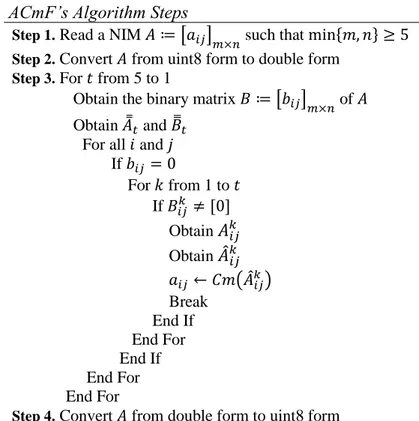
307 ACmF’s Algorithm Steps

Step 1. Read a NIM 𝐴 ≔ [𝑎_𝑖𝑗]

𝑚×𝑛 such that min{𝑚, 𝑛} ≥ 5

Step 2. Convert 𝐴 from uint8 form to double form Step 3. For 𝑡 from 5 to 1

Obtain the binary matrix 𝐵 ≔ [𝑏𝑖𝑗]_𝑚×𝑛 of 𝐴

Obtain 𝐴̿𝑡 and 𝐵̿𝑡

For all 𝑖 and 𝑗

If 𝑏𝑖𝑗= 0 For 𝑘 from 1 to 𝑡 If 𝐵𝑖𝑗𝑘 ≠ [0] Obtain 𝐴_𝑖𝑗𝑘 Obtain 𝐴̂_𝑖𝑗𝑘 𝑎𝑖𝑗 ← 𝐶𝑚(𝐴̂𝑖𝑗𝑘) Break End If End For End If End For End For

Step 4. Convert 𝐴 from double form to uint8 form

(5)

308

Finally, we discuss Adaptive Cesáro Mean Filter (ACmF), a novel filter. ACmF is recursive and uses the Cesàro mean instead of the standard median to assign a new value to the centre pixel of a window. Furthermore, if need be, it allows for the use of a bigger window size than those in DAMF. In other words, ACmF’s basic differences from DAMF are its recursive nature, its reliance on the Cesàro mean, and the use of window sizes up to 11 × 11. DAMF based on the standard median uses window sizes up to 7 × 7. ACmF produces new values closer to the original pixel values. However, although ACmF performs better than the state-of-art methods in terms of running time, it works a little slower due to the recursive procedure than DAMF does.

3. Simulation Results

In this section, we first present the quality metrics PSNR, SSIM, and MSSIM used to compare DBA, MDBUTMF, BPDF, NAFSMF, DAMF, AWMF, and ACmF. PSNR is defined as

𝑃𝑆𝑁𝑅(𝐸, 𝐹) ≔ 10log ( 255 2

𝑀𝑆𝐸(𝐸, 𝐹)) (5)

where MSE stands for the Mean Square Error and is defined as 𝑀𝑆𝐸(𝐸, 𝐹) ≔ 1 𝑚𝑛∑ ∑(𝑒𝑖𝑗 − 𝑓𝑖𝑗) 2 𝑛 𝑗=1 𝑚 𝑖=1 (6) Here, 𝐸 ≔ [𝑒_𝑖𝑗] is the earliest form/original image and 𝐹 ≔ [𝑓_𝑖𝑗] is the final form/restored image. SSIM [17] is defined as

𝑆𝑆𝐼𝑀(𝑥, 𝑦) ≔ (2𝜇𝑥𝜇𝑦+ 𝐶1) + (2𝜎𝑥𝑦+ 𝐶2) (𝜇𝑥2+ 𝜇𝑦2 + 𝐶1) + (𝜎𝑥2+ 𝜎𝑦2+ 𝐶2)

(7)

where 𝜇𝑥, 𝜇𝑦, 𝜎𝑥, 𝜎𝑦, and 𝜎𝑥𝑦 are the average intensities, standard deviations, and cross-covariance for images 𝑥 and 𝑦, respectively. Also, 𝐶₁ ≔ (𝐾₁𝐿)2 and 𝐶₂ ≔ (𝐾₂𝐿)2 are two constants such that 𝐾₁ = 0.01, 𝐾₂ = 0.03 and 𝐿 = 255 for 8-bit grayscale images.

MSSIM is defined as, for 𝑥₁, 𝑥₂, … , 𝑥_𝑛 and 𝑦₁, 𝑦₂, … , 𝑦_𝑛 images, 𝑀𝑆𝑆𝐼𝑀 ≔1

𝑛∑ 𝑆𝑆𝐼𝑀(𝑥𝑘, 𝑦𝑘) 𝑛

𝑘=1

(8)

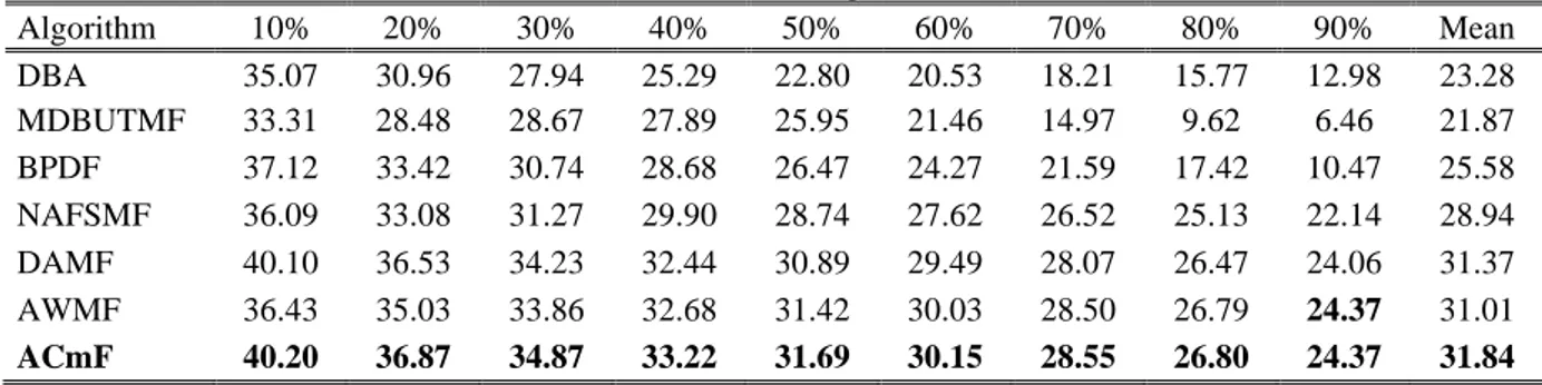
Secondly, we give mean PSNR and MSSIM results of the methods mentioned above for 15 traditional test images with 512×512 pixels (Baboon, Boat, Bridge, Cameraman, Elaine, Flintstones, Hill, House, Lake, Lena, Living Room, Parrot, Peppers, Pirate, and Plane) and 40 test images with 600×600 pixels in the TESTIMAGES Database [17] ranging in noise densities from 10% to 90%, in Table 1, 2, 3, and 4, respectively.

Table 1. Mean PSNR results for the 15 traditional images with different SPN ratios

Algorithm 10% 20% 30% 40% 50% 60% 70% 80% 90% Mean DBA 35.07 30.96 27.94 25.29 22.80 20.53 18.21 15.77 12.98 23.28 MDBUTMF 33.31 28.48 28.67 27.89 25.95 21.46 14.97 9.62 6.46 21.87 BPDF 37.12 33.42 30.74 28.68 26.47 24.27 21.59 17.42 10.47 25.58 NAFSMF 36.09 33.08 31.27 29.90 28.74 27.62 26.52 25.13 22.14 28.94 DAMF 40.10 36.53 34.23 32.44 30.89 29.49 28.07 26.47 24.06 31.37 AWMF 36.43 35.03 33.86 32.68 31.42 30.03 28.50 26.79 24.37 31.01 ACmF 40.20 36.87 34.87 33.22 31.69 30.15 28.55 26.80 24.37 31.84

(6)

309

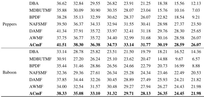
Table 2. MSSIM results for the 15 traditional images with different SPN ratios

Algorithm 10% 20% 30% 40% 50% 60% 70% 80% 90% Mean DBA 0.9655 0.9211 0.8613 0.7839 0.6910 0.5895 0.4846 0.3868 0.3154 0.6666 MDBUTMF 0.9425 0.7951 0.8387 0.8399 0.7835 0.6332 0.3254 0.0973 0.0213 0.5863 BPDF 0.9794 0.9552 0.9246 0.8857 0.8323 0.7628 0.6627 0.5008 0.2518 0.7506 NAFSMF 0.9753 0.9505 0.9246 0.8969 0.8662 0.8310 0.7891 0.7315 0.6087 0.8415 DAMF 0.9865 0.9714 0.9539 0.9332 0.9084 0.8789 0.8407 0.7887 0.6973 0.8843 AWMF 0.9737 0.9638 0.9507 0.9344 0.9134 0.8858 0.8477 0.7948 0.7039 0.8854 ACmF 0.9869 0.9732 0.9577 0.9395 0.9168 0.8881 0.8490 0.7954 0.7041 0.8901

Table 3. Mean PSNR results for the 40 images for TESTIMAGES Gallery with different SPN ratios

Algorithm 10% 20% 30% 40% 50% 60% 70% 80% 90% Mean DBA 36.68 31.97 28.40 25.32 22.53 19.72 17.03 14.21 11.27 23.01 MDBUTMF 30.19 26.49 26.88 26.33 24.48 20.35 14.48 9.44 6.33 20.55 BPDF 38.46 34.37 31.38 28.80 26.35 23.71 20.58 15.87 8.79 25.37 NAFSMF 37.20 34.14 32.14 30.55 29.22 27.91 26.50 24.83 21.34 29.31 DAMF 41.09 37.25 34.70 32.76 31.22 29.72 28.19 26.42 23.60 31.66 AWMF 37.56 36.53 35.45 34.26 32.90 31.38 29.66 27.67 24.85 32.25 ACmF 41.99 38.85 36.71 34.92 33.22 31.51 29.70 27.68 24.86 33.27

Table 4. MSSIM results for the 40 images for TESTIMAGES Gallery with different SPN ratios

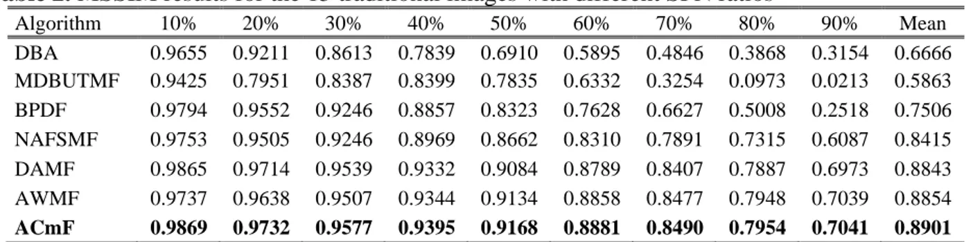
Algorithm 10% 20% 30% 40% 50% 60% 70% 80% 90% Mean DBA 0.9783 0.9451 0.8942 0.8221 0.7298 0.6179 0.4988 0.3793 0.2981 0.6849 MDBUTMF 0.9421 0.7728 0.8513 0.8792 0.8326 0.6850 0.3738 0.1326 0.0362 0.6117 BPDF 0.9853 0.9667 0.9411 0.9055 0.8562 0.7848 0.6782 0.4938 0.2065 0.7576 NAFSMF 0.9791 0.9601 0.9411 0.9207 0.8981 0.8716 0.8375 0.7869 0.6622 0.8730 DAMF 0.9910 0.9814 0.9697 0.9553 0.9379 0.9160 0.8869 0.8428 0.7567 0.9153 AWMF 0.9807 0.9748 0.9670 0.9568 0.9430 0.9234 0.8949 0.8510 0.7671 0.9176 ACmF 0.9914 0.9831 0.9734 0.9615 0.9462 0.9254 0.8960 0.8515 0.7672 0.9218 Thirdly, we give the PSNR and SSIM results of the methods for the images Cameraman, Lena, Peppers, and Baboon ranging in noise densities from 10% to 90%, in Table 5 and 6, respectively.

Table 5. PSNR results of the methods for some traditional images with different SPN ratios

Image Filters 10% 20% 30% 40% 50% 60% 70% 80% 90% Cameraman DBA 38.02 32.79 29.12 26.03 23.03 20.57 18.30 15.88 12.31 MDBUTMF 35.51 29.40 30.18 29.40 27.40 22.34 15.25 9.87 6.72 BPDF 39.62 35.30 32.19 29.81 27.37 24.73 22.28 18.32 11.50 NAFSMF 36.97 33.92 32.04 30.63 29.50 28.16 27.22 25.69 22.59 DAMF 43.90 39.49 36.75 34.50 32.92 31.10 29.56 27.71 24.89 AWMF 38.17 37.28 36.20 34.98 33.67 31.87 30.14 28.08 25.15 ACmF 43.87 40.38 37.95 35.91 34.16 32.03 30.20 28.09 25.15 Lena DBA 38.03 33.43 30.11 26.95 24.24 21.95 19.43 16.33 13.55 MDBUTMF 36.04 30.50 31.18 30.33 28.06 22.67 15.49 9.95 6.77 BPDF 39.88 35.82 32.86 30.51 28.37 25.89 23.01 18.01 10.84 NAFSMF 38.79 35.51 33.78 32.26 31.12 29.80 28.62 27.15 23.72 DAMF 43.12 39.07 36.66 34.90 33.24 31.77 30.18 28.56 25.88 AWMF 39.01 37.36 36.15 34.83 33.59 32.16 30.53 28.79 26.13 ACmF 42.52 39.11 37.09 35.40 33.85 32.28 30.57 28.80 26.13

(7)

310 Peppers DBA 36.62 32.84 29.55 26.82 23.91 21.25 18.38 15.56 12.13 MDBUTMF 35.88 30.09 30.90 30.35 28.07 23.04 15.76 10.16 7.03 BPDF 38.28 35.13 32.59 30.62 28.37 26.07 22.82 18.54 9.21 NAFSMF 39.50 36.37 34.33 32.94 31.55 30.41 28.98 27.37 23.50 DAMF 41.34 37.91 35.72 33.97 32.41 31.18 29.76 28.30 25.65 AWMF 37.75 36.77 35.72 34.40 32.99 31.68 30.16 28.58 26.07 ACmF 41.51 38.30 36.38 34.73 33.14 31.77 30.19 28.59 26.07 Baboon DBA 33.14 28.78 25.82 23.51 21.50 19.79 18.21 16.52 14.36 MDBUTMF 30.91 27.20 26.24 25.10 23.62 20.47 14.88 9.67 6.57 BPDF 35.44 31.46 28.86 26.56 24.66 22.79 20.73 16.99 8.88 NAFSMF 32.36 29.36 27.61 26.34 25.28 24.34 23.46 22.49 20.53 DAMF 37.85 34.44 32.26 30.45 28.89 27.49 25.93 24.21 21.82 AWMF 34.00 32.54 31.57 30.48 29.27 27.94 26.27 24.43 21.98 ACmF 38.33 35.08 33.10 31.32 29.71 28.13 26.35 24.45 21.98

Table 6. SSIM results of the methods for some traditional images with different SPN ratios

Image Filters 10% 20% 30% 40% 50% 60% 70% 80% 90% Cameraman DBA 0.9882 0.9656 0.9296 0.8774 0.8096 0.7321 0.6588 0.5883 0.4935 MDBUTMF 0.9548 0.7727 0.8755 0.9170 0.8821 0.7356 0.4051 0.1640 0.0555 BPDF 0.9914 0.9789 0.9601 0.9340 0.8936 0.8399 0.7698 0.6643 0.4885 NAFSMF 0.9804 0.9643 0.9493 0.9347 0.9184 0.8976 0.8732 0.8334 0.7176 DAMF 0.9962 0.9909 0.9842 0.9754 0.9650 0.9508 0.9313 0.9008 0.8370 AWMF 0.9879 0.9849 0.9810 0.9756 0.9682 0.9558 0.9367 0.9054 0.8421 ACmF 0.9964 0.9921 0.9870 0.9802 0.9713 0.9577 0.9378 0.9059 0.8422 Lena DBA 0.9761 0.9422 0.8963 0.8326 0.7528 0.6635 0.5656 0.4454 0.3587 MDBUTMF 0.9537 0.8154 0.8741 0.8840 0.8386 0.6830 0.3328 0.0866 0.0169 BPDF 0.9847 0.9656 0.9423 0.9105 0.8690 0.8117 0.7235 0.5391 0.2823 NAFSMF 0.9839 0.9665 0.9493 0.9293 0.9081 0.8813 0.8509 0.8038 0.6883 DAMF 0.9904 0.9787 0.9656 0.9497 0.9312 0.9081 0.8786 0.8384 0.7670 AWMF 0.9820 0.9737 0.9637 0.9504 0.9346 0.9129 0.8839 0.8433 0.7729 ACmF 0.9904 0.9795 0.9680 0.9536 0.9367 0.9143 0.8846 0.8436 0.7730 Peppers DBA 0.9537 0.9066 0.8477 0.7794 0.7018 0.6047 0.5031 0.3888 0.2789 MDBUTMF 0.9412 0.7865 0.8349 0.8429 0.7879 0.6538 0.3490 0.1140 0.0304 BPDF 0.9741 0.9472 0.9158 0.8814 0.8376 0.7792 0.6966 0.5583 0.1939 NAFSMF 0.9778 0.9555 0.9323 0.9080 0.8810 0.8517 0.8157 0.7663 0.6474 DAMF 0.9809 0.9601 0.9373 0.9121 0.8834 0.8514 0.8136 0.7679 0.6971 AWMF 0.9610 0.9557 0.9415 0.9212 0.8950 0.8633 0.8243 0.7759 0.7053 ACmF 0.9833 0.9652 0.9454 0.9230 0.8960 0.8637 0.8244 0.7758 0.7053 Baboon DBA 0.9660 0.9105 0.8294 0.7230 0.6002 0.4709 0.3519 0.2500 0.1955 MDBUTMF 0.9390 0.8307 0.8113 0.7689 0.6908 0.5451 0.2895 0.0790 0.0119 BPDF 0.9796 0.9508 0.9119 0.8564 0.7833 0.6855 0.5550 0.3814 0.1059 NAFSMF 0.9613 0.9202 0.8779 0.8318 0.7802 0.7212 0.6533 0.5731 0.4433 DAMF 0.9885 0.9743 0.9575 0.9359 0.9084 0.8744 0.8228 0.7475 0.5973 AWMF 0.9721 0.9602 0.9494 0.9346 0.9133 0.8832 0.8323 0.7555 0.6037 ACmF 0.9898 0.9778 0.9643 0.9463 0.9218 0.8888 0.8355 0.7570 0.6043

(8)

311

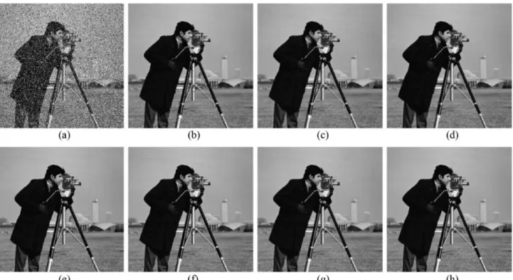
Fourthly, we give PSNR and SSIM results of DBA, MDBUTMF, BPDF, NAFSMF, DAMF, AWMF, and ACmF for the image Cameraman with a noise density of 30%, in Figure 2.

Figure 2. PSNR and SSIM results for “Cameraman” of size 512 × 512 with SPN ratio of 30%. (a) Noisy image (10.31, 0.0550), (b) DBA (29.12, 0.9296), (c) MDBUTMF (30.18, 0.8755), (d) BPDF (32.19, 0.9601), (e) NAFSMF (32.04, 0.9493), (f) DAMF (36.75, 0.9842), (g) AWMF (36.20, 0.9810), (h) ACmF (37.95, 0.9870)

Fifthly, we then give PSNR and SSIM results of ACmF for the image Lena ranging in noise densities from 10% to 90%, in Figure 3.

Figure 3. PSNR and SSIM results of ACmF for “Lena” of size 512 × 512 with different SPN ratios. (a) 10% (15.40, 0.1704) (b) 30% (10.67, 0.0529) (c) 50% (8.47, 0.0264) (d) 70% (6.98, 0.0126) (e) 90% (5.90, 0.0064) (f) Removed 10% (42.52, 0.9904) (g) Removed 30% (37.09, 0.9680) (h) Removed 50% (33.85, 0.9367) (i) Removed 70% (30.57, 0.8846) (j) Removed 90% (26.13, 0.7730)

(9)

312

Sixthly, we give the PSNR graph for the images: Almonds, Bananas, Billiard Balls A, Guitar Bridge, Building, and Cushions, which is in TESTIMAGES Database, ranging in noise densities from 10% to 90%, in Fig. 4. According to these results, ACmF is a more successful method than the others in any noise densities.

Figure 4. PSNR Graphs, (a) Almonds (b) Bananas (c) Billiard Balls A (d) Guitar Bridge (e) Building

(f) Cushions.

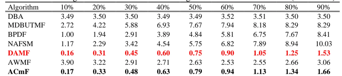
Finally, we give the running time data of the algorithms in Table 7 and 8 for 15 traditional images and TESTIMAGES database with different SPN ratios, respectively. Here, we use MATLAB R2019a and a workstation with I(R) Xeon(R) CPU E5-1620 v4 @ 3.5 GHz and 64 GB RAM for these comparisons. The results show that ACmF outperforms the methods mentioned above except for DAMF in terms of running time. Moreover, ACmF is much more successful NAFSMF and AWMF, which are known as successful in high noise densities.

Table 7. Mean running time for the 15 traditional images with different SPN ratios (in Seconds)

Algorithm 10% 20% 30% 40% 50% 60% 70% 80% 90% DBA 3.49 3.50 3.50 3.49 3.49 3.52 3.51 3.50 3.50 MDBUTMF 2.72 4.22 5.88 6.93 7.67 7.94 8.18 8.29 8.29 BPDF 1.00 1.94 2.91 3.89 4.84 5.81 6.75 7.67 8.41 NAFSM 1.17 2.29 3.42 4.54 5.75 6.82 7.89 8.94 10.03 DAMF 0.16 0.31 0.45 0.60 0.75 0.90 1.05 1.25 1.53 AWMF 3.90 3.22 2.91 2.71 2.63 2.53 2.55 2.66 3.06 ACmF 0.17 0.33 0.48 0.63 0.79 0.94 1.13 1.34 1.66

Table 8. Mean running time for the 40 images with different SPN ratios (in Seconds)

Algorithm 10% 20% 30% 40% 50% 60% 70% 80% 90% DBA 4.78 4.79 4.80 4.81 4.81 4.80 4.80 4.78 4.78 MDBUTMF 3.77 5.83 8.12 9.52 10.35 10.85 11.17 11.33 11.31 BPDF 1.44 2.73 4.02 5.33 6.61 7.88 9.16 10.46 11.58 NAFSM 1.70 3.23 4.75 6.29 7.80 9.30 10.80 12.24 13.67 DAMF 0.23 0.43 0.63 0.83 1.04 1.23 1.44 1.70 2.10 AWMF 5.36 4.35 3.91 3.65 3.59 3.44 3.47 3.68 4.33 ACmF 0.25 0.46 0.67 0.87 1.11 1.30 1.55 1.83 2.30

(10)

313

5. Conclusion

In the present paper, we proposed ACmF, an efficient filter for SPN removal, and showed that ACmF performs better than the known methods for all noise densities. ACmF uses the Cesáro mean of regular pixels as opposed to DAMF using the median. Moreover, ACmF is recursive and, if needed, allows for the use of a bigger window size than those in DAMF. We compared ACmF with the state-of-art methods whose algorithms were accessible. We, in this paper, did not consider the filters whose algorithms were not accessible either on private or on global platforms, such as MathWorks. Further, ACmF can be developed by exploiting a weighted mean or by employing a noise detection mask. This concept has first been presented in [21] as an abstract. Since ACmF produces the best results in any noise density, it can be clearly observed that ACmF outperforms the others. On the other hand, determining the ranking order of the other filters is not easy. Therefore, obtaining their ranking order is another crucial topic. For more details, see [22-26].

Acknowledgements

This work was supported by the Office of Scientific Research Projects Coordination at Çanakkale Onsekiz Mart University, Grant number: FHD-2018-1409.

References

[1] Erkan U., Enginoğlu S., Thanh D. N. H., "A Recursive Mean Filter for Image Denoising", IEEE 2019 International Conference on Artificial Intelligence and Data Processing, Malatya, Turkey, 1-5, (2019). [2] Thanh D. N. H., Thanh L. T., Surya Prasath V. B., Erkan U., "An Improved BPDF Filter for High Density

Salt and Pepper Denoising", IEEE-RIVF International Conference on Computing and Communication Technologies (RIVF), Danang, Vietnam, 1-5, (2019).

[3] Erkan U., Gökrem L., Enginoğlu S., "Adaptive Right Median Filter for Salt-and-Pepper Noise Removal", International Journal of Engineering Research and Development, 2019, 11(2): 542-550.

[4] Erkan, U, Thanh, D. N. H., Hieu L. M., Enginoğlu, S., "An Iterative Mean Filter for Image Denoising", IEEE Access, 2019, 7: 167847-167859.

[5] Enginoğlu S., Erkan U., Memiş S., "Pixel Similarity-Based Adaptive Riesz Mean Filter for Salt-and-Pepper Noise Removal", Multimedia Tools and Applications, 2019, 78(24): 35401-35418.

[6] Thanh D., Surya Prasath V. B., Hieu L. M., "A Review on CT and X-Ray Images Denoising Methods", Informatica, 2019, 43: 151-159.

[7] Thanh D. N. H., Surya Prasath V. B., Thanh, L. T., "Total Variation L1 Fidelity Salt-and-Pepper Denoising with Adaptive Regularization Parameter", 5th NAFOSTED Conference on Information and Computer Science (NICS), Ho Chi Minh City, Vietnam, 400-405, (2018).

[8] Tukey J. W., "Exploratory Data Analysis", Ed: Frederick Mosteller, Addison-Wesley Publishing Company, (1977).

[9] Pratt W. K., "Semiannual Technical Report", Image Processing Institute, University of Southern California, (1975).

[10] Hwang H., Haddad R. A., "Adaptive Median Filters: New Algorithms and Results", IEEE Transactions on Image Processing, 1995, 4(4): 499-502.

[11] Erkan U., Gökrem L., "Median Filter without Repetition in Salt and Peppers Noise", Gaziosmanpasa Journal of Scientific Research, 2017, 6(2): 11-19.

[12] Wang Z., Zhang D., "Progressive Switching Median Filter for the Removal of Impulse Noise from Highly Corrupted Images", IEEE Transactions on Circuits and Systems II Analog and Digital Signal Processing, 1999, 46(1): 78-80.

[13] Pattnaik A., Agarwal S., Chand S., "A New and Efficient Method for Removal of High Density Salt and Pepper Noise Through Cascade Decision based Filtering Algorithm", Procedia Technology, 2012, 6: 108-117.

(11)

314

[14] Esakkirajan S., Veerakumar T., Subramanyam A. N., PremChand, C. H., "Removal of High Density Salt and Pepper Noise Through Modified Decision Based Unsymmetric Trimmed Median Filter", IEEE Signal Processing Letters, 2011, 18(5): 287-290.

[15] Toh K. K. V., Isa N. A. M., "Noise Adaptive Fuzzy Switching Median Filter for Salt-and-Pepper Noise Reduction", IEEE Signal Processing Letters, 2010, 17(3): 281-284.

[16] Erkan U., Kılıçman A., "Two New Methods for Removing Salt-and-Pepper Noise from Digital Images", Science Asia, 2016, 42: 28-32.

[17] Wang Z., Bovik A. C., Sheikh H. R., Simoncelli E. P., "Image Quality Assessment: From error Visibility to Structural Similarity", IEEE Transactions on Image Processing, 2004, 13(4): 600-612.

[18] Erkan U., Gökrem L., "A New Method Based on Pixel Density in Salt and Pepper Noise Removal", Turkish Journal of Electrical Engineering and Computer Sciences, 2018, 26: 162-171.

[19] Erkan U., Gökrem L., Enginoğlu S., "Different Applied Median Filter in Salt and Pepper Noise", Computer and Electrical Engineering, 2018, 70: 789-798.

[20] Zhang P., Li F., "A New Adaptive Weighted Mean Filter for Removing Salt-and-Pepper Noise", IEEE Signal Processing Letters, 2014, 21(10): 1280-1283.

[21] Enginoğlu S., Erkan U., Memiş S., "Adaptive Cesáro Mean Filter for Salt-and-Pepper Noise Removal", ICONST EST 2019 International Conferences on Science and Technology Engineering Science and Technology, Prizren, Kosovo, 37 (2019).

[22] Enginoğlu S., Memiş S., "Comment on Fuzzy soft sets [The Journal of Fuzzy Mathematics, 9(3), 2001, 589–602]", International Journal of Latest Engineering Research and Applications, 2018, 3(9): 1-9. [23] Enginoğlu S., Memiş S., Arslan B., "Comment (2) on Soft Set Theory and uni-int Decision Making

[European Journal of Operational Research, (2010) 207, 848-855]", Journal of New Theory, 2018, 25: 85-102.

[24] Enginoğlu S., Memiş S., Öngel T., "Comment on Soft Set Theory and Uni-Int Decision Making [European Journal of Operational Research, (2010) 207, 848-855]", Journal of New Results in Science, 2018, 7(3): 28-43.

[25] Enginoğlu S., Memiş S., Çağman N., "A Generalisation of Fuzzy Soft Max-Min Decision-Making Method and Its Application to A Performance-Based Value Assignment in Image Denoising", El-Cezerî Journal of Science and Engineering, 2019, 6(3): 466-481.

[26] Enginoğlu S., Memiş S., Karaaslan F., "A New Approach to Group Decision-Making Method Based on TOPSIS Under Fuzzy Soft Environment", Journal of New Results in Science, 2019, 8(2): 42-52.