Estimation in the Complementary Exponential Geometric
Distribution Based on Progressive Type‑II Censored Data
Özlem Gürünlü Alma1 · Reza Arabi Belaghi2
Received: 15 July 2017 / Revised: 12 November 2018 / Accepted: 19 March 2019 / Published online: 26 July 2019
© School of Mathematical Sciences, University of Science and Technology of China and Springer-Verlag GmbH Germany, part of Springer Nature 2019
Abstract
Complementary exponential geometric distribution has many applications in survival and reliability analysis. Due to its importance, in this study, we are aiming to estimate the parameters of this model based on progressive type-II censored observations. To do this, we applied the stochastic expectation maximization method and Newton–Raphson tech-niques for obtaining the maximum likelihood estimates. We also considered the estimation based on Bayesian method using several approximate: MCMC samples, Lindely approxi-mation and Metropolis–Hasting algorithm. In addition, we considered the shrinkage esti-mators based on Bayesian and maximum likelihood estiesti-mators. Then, the HPD intervals for the parameters are constructed based on the posterior samples from the Metropolis– Hasting algorithm. In the sequel, we obtained the performance of different estimators in terms of biases, estimated risks and Pitman closeness via Monte Carlo simulation study. This paper will be ended up with a real data set example for illustration of our purpose. Keywords Bayesian analysis · Complementary exponential geometric (CEG) distribution · Progressive type-II censoring · Maximum likelihood estimators · SEM algorithm · Shrinkage estimator
Mathematics Subject Classification 62N01 · 62N02 1 Introduction
Complementary risk (CR) problems arise naturally in a number of context, especially in problem of survival analysis, actuarial science, demography and industrial reliability * Özlem Gürünlü Alma
[email protected] Reza Arabi Belaghi [email protected]
1 Department of Statistics, Faculty of Sciences, Muğla Sıtkı Koçman University, Muğla, Turkey 2 Department of Statistics, Faculty of Mathematical Sciences, University of Tabriz, Tabriz, Iran
[6]. In the classical complementary risk scenarios, the event of interest is related to causes which are not completely observed. Therefore, the lifetime of the event of interest is modeled as function of the available information, which is only the maximum ordered lifetime value among all causes. In the presence of CR in survival analysis, the risks are latent in the sense that there is no information about which factor was responsible for component failure, we observe only the maximum lifetime value among all risks. For example, when studying death on dialysis, receiving a kidney transplant is an event that competes with the event of interest such as heart failure, pulmonary embolism and stroke. In reliability, it observed only the maximum component lifetime of a parallel system, that is, the observable quantities for each component are the maximum lifetime value to failure among all risks and the cause of failure. For instance, in industrial applications, the failure of a device can be caused by several competing causes such as the failure of a component, contamination from dirt, an assembly error, harsh working environments, among others. For more literature on complementary risk problems, we refer the reader to Cox and Oakes [10], Crowder et al. [9], Goetghebeur and Ryan [14], Reiser et al. [34], Lawless [22] and Lu and Tsiatis [27, 28].
The complementary exponential geometric (CEG) model is derived as follows. Let M be a random variable denoting the number of failure causes, m = 1, 2, … , and considering M with geometrical distribution of probability given by
Let us consider xi, i= 1, 2, … , realizations of random variable denoting the failure
times, i.e., the time to event due to the i th complementary risk, with Xi has an
exponen-tial distribution with probability index 𝜆 , given by
In the latent complementary risk scenario, the number of causes M and the lifetime xi associated with a particular cause are not observable (latent variables), and only the maximum lifetime X among all causes is usually observed. So, it is only observed that the random variable is given by
The CEG distribution, proposed recently by Louzada et al. [26] is useful model for modeling lifetime data. This distribution, with increasing failure rate, is complementary to the exponential geometric model given by Adamidis and Loukas [1]. Louzada et al. [26] showed that the probability distribution function of the two-parameter CEG ran-dom variables X is given by
where x > 0, 𝜆 > 0 and 0 < 𝜃 < 1 . Here 𝜆 and 𝜃 are the scale and shape parameters, respectively. It is denoted as X ∼ CEG(𝜆, 𝜃) . The cumulative distribution function (CDF) and survival function of the CEG(𝜆, 𝜃) are given by
P(M = m) = 𝜃(1 − 𝜃)m−1, 0 < 𝜃 < 1, M= 1, 2, … . f(xi;𝜆 ) = 𝜆 exp{−𝜆xi } . X= max{Xi, 1≤ i ≤ M } . (1.1) f(x;𝜆, 𝜃) = 𝜆𝜃e −𝜆x [ e−𝜆x(1 − 𝜃) + 𝜃]2 , (1.2) F(x;𝜆, 𝜃) = 1 − e −𝜆x [ e−𝜆x(1 − 𝜃) + 𝜃],
respectively.
Where the lifetime associated with a particular risk is not observable, and it observed only the maximum lifetime value among all risks, then this distribution is used in latent complementary risks scenarios. Louzada et al. [26] discussed many properties of this model. But, they did not study about the estimation of the param-eters based on censored data and prediction of future-order statistics. So, in this paper, we are aiming to cover these.
The rest of the paper is as follows: In Sect. 2, we discuss the maximum likelihood estimators of the parameters based on an expectation maximization (EM) and sto-chastic EM (SEM) algorithm. Section 3 deals with Bayes and shrinkage Bayes esti-mations assuming the Gamma and Beta priors. Prediction intervals for the survival time of future observation are also given in this section. Simulation studies as well as an illustrative example are the content of Sect. 4, and we gave our conclusion and the results in Sect. 5.
2 Maximum Likelihood Estimation
In this section, we determined the maximum likelihood estimates (MLEs) of the parameters of CEG distribution based on progressive type-II censored samples.
Suppose that n independent units are put on a test and that the lifetime distri-bution of each unit is given by f(xj;𝜆, 𝜃) . Now consider the problem, the ordered m failures are observed under the progressively type-II censoring scheme plan R=(R
1,… , Rm
)
, where each Rj≥ 0 ,
∑m
j=1Rj+ m = n . If the ordered m failures are
denoted by X1∶m∶n<X2∶m∶n<… < Xm∶m∶n , then the likelihood function based on the observed sample X =(X1∶m∶n, X2∶m∶n,… , Xm∶m∶n
) is given by where c = n�n− 1 − R1��n− 2 − R1− R2�… � n−∑mj=1−1Rj− m + 1 � . For simplic-ity, we denoted xj∶m∶n by xj , j = 1, … , m . Then, from Eqs. (1.1), (1.2) and (2.1), we
can write the log-likelihood function of 𝜆 and 𝜃 based on progressive type-II cen-sored observed sample x as:
(1.3) S(x;𝜆, 𝜃) = e −𝜆x [ e−𝜆x(1 − 𝜃) + 𝜃], (2.1) L(x;𝜆, 𝜃) = c m ∏ j=1 f(xj;𝜆, 𝜃 )[ 1− F(xj;𝜆, 𝜃 )]Rj , (2.2) l(x;𝜆, 𝜃) ∝ m ln (𝜆) + m ln (𝜃) − 𝜆 m ∑ j=1 xj − 2 m ∑ j=1 ln[e−𝜆xj(1 − 𝜃) + 𝜃]+ m ∑ j=1 Rjln [ e−𝜆xj e−𝜆xj(1 − 𝜃) + 𝜃 ] .
MLEs of the parameters 𝜆 and 𝜃 can be obtained by solving two nonlinear equations simultaneously. In most cases, the estimators do not admit explicit. They have to be obtained by solving a two-dimensional optimization problem. It is observed that the standard Newton–Raphson (NR) algorithm has some problems such as does not converge in certain cases, a biased procedure, very sensitive to the initial values and also if the missing data are large then it is not convergent [31]. Little and Rubin [25] demonstrated that the estimation and maximization (EM) algorithm though converges slowly but is reasonably more reliable compared to the Newton–Raphson method, particularly when the missing data are relatively large. Here, we suggest using the EM algorithm to compute the desired MLEs.
2.1 EM and SEM Algorithm
The EM algorithm, originally proposed by Dempster et al. [12], is a very power-ful tool in handling the incomplete data problem. The EM algorithm has two steps, E-step and M-step. For the E-step, one needs to compute the pseudo-log-likelihood function. It can be emerged from 𝜄(w;𝜆, 𝜃) by substituting any function of zjk say g
( zjk ) with E[g(zjk ) |zjk>xj ]
. And in the M-step, E(log 𝜄(w;𝜆, 𝜃)) is maximized by taking the derivatives with respect to the parameters. McLachlan and Krishnan [30] gave a detailed discussion on EM algorithm and its applications.
We treat this problem as a missing value problem similarly as in Ng et al. [31]. The progressive type-II censoring can be viewed as an incomplete data set, and therefore, an EM algorithm is a good alternative to the NR method for numerically finding the MLEs. First, let us consider the observed and the censored data by X=(X
1∶m∶n,… , Xm∶m∶n )
and Z =(Z1,… , Zm) , respectively, where each Zj is 1 × Rj
vector with Zj=
(
Zj1,… , ZjRj
)
for j = 1, … , m, and they are not observable. The cen-sored data vector Z can be thought of as missing data. The combination of W = (X, Z) forms the complete data set. The log-likelihood (LL) function based on the complete data is
The MLEs of the parameters 𝜆 and 𝜃 for complete sample w can be obtained by deriving the log-likelihood function in Eq. (2.3) with respect to 𝜆 and 𝜃 and equating the normal equations to 0 as follows:
(2.3) LL(w;𝜆, 𝜃) ∝ n ln 𝜆 + n ln 𝜃 − 𝜆 m ∑ j=1 xj− 2 m ∑ j=1 ln[e−𝜆xj(1 − 𝜃) + 𝜃] − 𝜆 m ∑ j=1 Rj ∑ k=1 zjk2 m ∑ j=1 Rj ∑ k=1 ln[e−𝜆zjk(1 − 𝜃) + 𝜃].
In the E-step, the pseudo-log-likelihood function becomes,
We need the following result in sequel.
Theorem 2.1 Given X1 = x1,… , Xj= xj , the conditional distribution of Zjk ,
k= 1, … , Rj , has form
where zj>xj and 0 otherwise.
Proof The proof is straight forward. For details, see Ng et al. [31]. Using Theo-rem 2.1, we can write
And, 𝜕LL(w;𝜆, 𝜃) 𝜕𝜆 = n 𝜆− m ∑ j=1 xj+ 2 m ∑ j=1 xje−𝜆xj(1 − 𝜃) e−𝜆xj(1 − 𝜃) + 𝜃− m ∑ j=1 Rj ∑ k=1 zjk+ 2 m ∑ j=1 Rj ∑ k=1 zjke−𝜆zjk(1 − 𝜃) e−𝜆zjk(1 − 𝜃) + 𝜃 = 0, 𝜕LL(w;𝜆, 𝜃) 𝜕𝜃 = n 𝜃− 2 m ∑ j=1 1− e−𝜆xj e−𝜆xj(1 − 𝜃) + 𝜃− 2 m ∑ j=1 Rj ∑ k=1 1− e−𝜆zjk e−𝜆zjk(1 − 𝜃) + 𝜃 = 0. (2.4) 𝜕LL(w;𝜆, 𝜃) 𝜕𝜆 = n 𝜆− m ∑ j=1 xj+ 2 m ∑ j=1 xje−𝜆xj(1 − 𝜃) e−𝜆xj(1 − 𝜃) + 𝜃 − m ∑ j=1 Rj ∑ k=1 E[zjk|zjk>xj] + 2 m ∑ j=1 Rj ∑ k=1 E [ zjke−𝜆zjk(1 − 𝜃) e−𝜆zjk(1 − 𝜃) + 𝜃|zjk >xj ] = 0, (2.5) 𝜕LL(w;𝜆, 𝜃) 𝜕𝜃 = n 𝜃− 2 m ∑ j=1 1− e−𝜆xj e−𝜆xj(1 − 𝜃) + 𝜃 − 2 m ∑ j=1 Rj ∑ k=1 E [ 1− e−𝜆zjk e−𝜆zjk(1 − 𝜃) + 𝜃|zjk >xj ] = 0. (2.6) fZ|X ( zj|X1= x1,… , Xj= xj ) = fZ|X ( zj|Xj= xj ) = f(zj|𝜆, 𝜃) [1 − F(xj|𝜆, 𝜃)] , (2.7) E1 = E[Zjk|Zjk>xj]= 𝜆𝜃 1− F(xj|𝜆, 𝜃) × ∫ ∞ xj zjke−𝜆zj[e−𝜆zj(1 − 𝜃) + 𝜃]−2dz j. E2 = E [ zjke−𝜆zjk(1 − 𝜃) e−𝜆zjk(1 − 𝜃) + 𝜃|Zjk >xj ]
And,
Thus, in the M-step of the (k + 1) th nonlinear iteration of the EM algorithm, the value of 𝜆(k+1) is first obtained by solving the following equation:
Once 𝜆(k+1) is obtained, then 𝜃(k+1) is obtained by solving the equation
(
𝜆(k+1), 𝜃(k+1)) is then used as the new value of (𝜆, 𝜃) in the subsequent iteration. Now the desired maximum likelihood estimates of 𝜆 and 𝜃 can be obtained using an itera-tive procedure which continues until ||𝜆(k+1)− 𝜆(k)|| + ||𝜃(k+1)− 𝜃(k)|| < 𝜀 , for some k , and a prespecified small value of 𝜀.
A typical EM algorithm iteratively applies two steps; it is often having a simple closed form. However, in particular with high-dimensional data or increasing complexity for censored and lifetime models, one of the biggest disadvantages of EM algorithm is that it is only a local optimization procedure and can easily get stuck in a saddle point [40]. A possible solution to overcome the computational inefficiencies is to invoke stochastic EM algorithm suggested by Celeux and Diebolt [7], Nielsen [32] and Arabi Belaghi et al. [4]. It can be seen that the above EM expressions do not turn out to have closed form and therefore one needs to compute these expressions numerically. So, we used SEM algorithm to obtain maximum likelihood estimators.
The SEM algorithm is a two-step approach: the stochastic imputation step (S-step) and the maximization step (M-step). The main idea of the SEM algorithms is to replace the E-step by a stochastic step where the missing data Z are imputed with a single draw from the distribution of the missing data conditional on the (2.8) E2= 𝜆𝜃 1− F(xj|𝜆, 𝜃)× ∫ ∞ xj zjke−𝜆zjk(1 − 𝜃) [ e−𝜆zjk(1 − 𝜃) + 𝜃] e−𝜆zj [ e−𝜆zj(1 − 𝜃) + 𝜃]2 dzj. (2.9) E3= E [ 1− e−𝜆zjk e−𝜆zjk(1 − 𝜃) + 𝜃|Zjk >xj ] = 𝜆𝜃 1− F(xj|𝜆, 𝜃)× ∫ ∞ xj ( 1− e−𝜆zjk) [ e−𝜆zjk(1 − 𝜃) + 𝜃] × e −𝜆zj [ e−𝜆zj(1 − 𝜃) + 𝜃]2 dzj. 𝜕LL(w;𝜆, 𝜃) 𝜕𝜆 = n 𝜆(k+1) − m ∑ j=1 xj+ 2 m ∑ j=1 xje−𝜆(k+1)xj(1− 𝜃(k)) e−𝜆(k+1)xj(1− 𝜃(k))+ 𝜃(k) − m ∑ j=1 RjE1(xj;𝜆(k), 𝜃(k))+ 2 m ∑ j=1 RjE2(xj;𝜆(k), 𝜃(k))= 0. 𝜕LL(w;𝜆, 𝜃) 𝜕𝜃 = n 𝜃(k+1)− 2 m ∑ j=1 1− e−𝜆(k+1)x j e−𝜆(k+1)xj(1− 𝜃(k+1))+ 𝜃(k+1)− 2 m ∑ j=1 RjE3 ( xj;𝜆(k+1), 𝜃(k) ) = 0,
observed X. The Z is then substituted to (2.3) to form the pseudo 𝜄(w;𝜆, 𝜃) function, which is the optimized in the M-step to obtain (𝜆k+1, 𝜃k+1) for the next cycle. These two steps are repeated iteratively until a stationary distribution is reached for each parameter. The mean of this stationary distribution is considered as an estimator for the parameters. More formally, given the parameter estimate (𝜆k, 𝜃k) at the kth SEM
cycle, (k + 1)st cycle of the SEM algorithm evolves as follows: S-Step Given the current (𝜆k, 𝜃k) , simulate (R
j
)
independent values from the con-ditional distribution fZ|X
(
xj∶m∶n;𝜆, 𝜃) , respectively, for j = 1, … , m to form a realiza-tion of Z.
M-Step Maximize the pseudo 𝜄(w;𝜆, 𝜃) function given (X, Z) to obtain (
𝜆k+1, 𝜃k+1). □
2.2 Fisher Information Matrix
In this section, we present the observed Fisher information matrix obtained using the missing value principle of Louis [29]. The observed Fisher information matrix can be used to construct the asymptotic confidence intervals. The idea of missing information principle is as follows:
Let us use the following notation (regardless of denoting by bold notation): 𝜂= (𝜆, 𝜃) , X : the observed data, W : the complete data, IW(𝜂) : the complete information, IX(𝜂) : the observed information and IW|X(𝜂) : the missing information.
Then, they can be expressed as follows: The complete information IW(𝜂) is given by
The Fisher information matrix of the censored observations can be written as fZ|X ( xj∶m∶n;𝜆, 𝜃 ) = f ( zjk;𝜆, 𝜃 ) 1− F(xj∶m∶n;𝜆, 𝜃 ) or fZ|X ( xj∶m∶n;𝜆, 𝜃 ) =F ( zjk;𝜆, 𝜃 ) − F(xj∶m∶n;𝜆, 𝜃 ) 1− F(xj∶m∶n;𝜆, 𝜃 ) (2.10) Observed information= Complete information − Missing information.
(2.11) IX(𝜂) = IW(𝜂) − IW|X(𝜂). IW(𝜂) = −E [ 𝜕2𝜄(W;𝜂) 𝜕𝜂2 ] . IW(j)|X(𝜂) = −EZ j|Xj [ 𝜕2ln fZj(zj|Xj, 𝜂) 𝜕𝜂2 ] , IW|X(𝜂) = m ∑ j=1 RjIW(j)|X(𝜂).
So we obtain the observed information as
And naturally, the asymptotic variance covariance matrix of ̂𝜂 can be obtained by inverting IX( ̂𝜂) . The elements of matrices for IW(𝜂) and IW|X(𝜂) are denoted by aij(𝜆, 𝜃)
and bij(𝜆, 𝜃).They are as follows:
Now we provide IW|X(𝜂) . Since
In which,
Note that, we use the plug-in method of MLEs of 𝜆 and 𝜃 in finding the above val-ues. Consequently the variance–covariance matrix of parameter 𝜂 can be obtained by
Observe that we still need to obtain the integrations which may be cumbersome task. Next, we use the SEM algorithm to compute observed information matrix. We first generate the censored observations zij using Monte Carlo simulation from the
condi-tional density as discussed in before. Subsequently the asymptotic variance–covariance matrix of the MLEs of the parameters can be obtained. Therefore, an approximate (1 − 𝛼)100% confidence interval for 𝜆 and 𝜃 is obtained as ̂𝜆 ± z𝛼∕
2 √ ̂ V(𝜆̂) and IX(𝜂) = IW(𝜂) − IW|X(𝜂). a11= n 𝜆2 + 2n𝜆𝜃 2 (1 − 𝜃) ∫ ∞ 0 x2e−2𝜆x [ e−𝜆x(1 − 𝜃) + 𝜃]4dx. a22= n 𝜃2 − 2n𝜆𝜃 ∫ ∞ 0 e−𝜆x[1− e−𝜆x]2 [ e−𝜆x(1 − 𝜃) + 𝜃]4 dx. a12= a21= 2n𝜆𝜃 ∫ ∞ 0 xe−2𝜆x [ e−𝜆x(1 − 𝜃) + 𝜃]4dx. IW|X(𝜂) = m ∑ j=1 Rj [ b11(xj;𝜆, 𝜃 ) b12(xj;𝜆, 𝜃 ) b21(xj;𝜆, 𝜃) b22(xj;𝜆, 𝜃) ] . b11(xj;𝜆, 𝜃)= 1 𝜆2− x2je−𝜆xj𝜃(1 − 𝜃) [ e−𝜆xj(1 − 𝜃) + 𝜃]2 + 2𝜆𝜃2 (1 − 𝜃) ∫ ∞ 0 z2je−2𝜆zj [ e−𝜆zj(1 − 𝜃) + 𝜃]4 dzj. b22(xj;𝜆, 𝜃)= 1 𝜃2+ [ 1− e−𝜆xj]2 [ e−𝜆xj(1 − 𝜃) + 𝜃]2 − 2𝜆𝜃 ∫ ∞ 0 e−𝜆zj[1− e−𝜆zj]2 [ e−𝜆zj(1 − 𝜃) + 𝜃]4 dzj. b12(xj;𝜆, 𝜃)= b21(xj;𝜆, 𝜃)= − xje −𝜆xj [ e−𝜆xj(1 − 𝜃) + 𝜃]2+ 2𝜆𝜃 ∫ ∞ 0 zje−2𝜆zj [ e−𝜆zj(1 − 𝜃) + 𝜃]4 dzj. (2.12) IX−1(𝜂) =[IW(𝜂) − IW|X(𝜂) ]−1 .
̂ 𝜃± z𝛼∕ 2 √ ̂ V(𝜃̂) , where z𝛼 ∕2 is the (𝛼∕ 2 )
100 th percentile of standard normal distribution.
3 Bayes Estimates
In this section, we consider the Bayes estimates of the unknown parameters. For a Bayesian estimation of the parameters, one needs prior distributions for these parameters. These prior distributions depend upon the knowledge about the param-eters and the experience of similar phenomena. When both the paramparam-eters of the model are unknown, a joint conjugate prior for the parameters does not exist. In view of the above, we propose to use independent gamma and beta priors for 𝜆 and 𝜃 , respectively. So, we assume the following independent priors:
Here, all the hyper-parameters a1, b1, a2, b2 are assumed to be known and non-negative. It can be observed that the non-informative priors of the parameters are the special case of the proposed prior distribution. Based on the observed sample {
x1∶m∶n,… , xm∶m∶n }
, from the progressive type-II censoring scheme, the likelihood function becomes:
The joint posterior density functions of 𝜆 and 𝜃 can be written as
where
One may use the importance sampling method to obtain the MCMC samples and then compute the Bayes estimates. The simulation algorithm based on importance sampling is as follows. (3.1) 𝜋1(𝜆) ∝ 𝜆a1−1e−b1𝜆, 𝜆 >0, (3.2) 𝜋2(𝜃) ∝ 𝜃a2−1(1 − 𝜃)b2−1, 0 < 𝜃 < 1. (3.3) l(X;𝜆, 𝜃) ∝ 𝜆m𝜃m e−𝜆∑mj=1xje−2 ∑m j=1ln � e−𝜆xj(1−𝜃)+𝜃 � e ∑m j=1Rjln � e−𝜆xj e−𝜆xj(1−𝜃)+𝜃 � . (3.4) 𝜋(𝜆, 𝜃�x) ∝ 𝜆m+a1−1e−𝜆 �∑m j=1xj+b1 � 𝜃m+a2−1(1 − 𝜃)b2−1e−2 ∑m j=1ln � e−𝜆xj(1−𝜃)+𝜃� × e ∑m j=1Rjln � e−𝜆xj e−𝜆xj(1−𝜃)+𝜃 � = 𝜆m+a1−1e−𝜆 �∑m j=1xj+b1+∑mj=1Rjxj � 𝜃m+a2−1(1 − 𝜃)b2−1e−2 ∑m j=1ln � e−𝜆xj(1−𝜃)+𝜃 � × e− ∑m j=1Rjln � e−𝜆xj(1−𝜃)+𝜃� = gamma � m+ a1, b1+ m � j=1 xj+ m � j=1 Rjxj � × Beta�m+ a2, b2 � × h(𝜆, 𝜃), h(𝜆, 𝜃) = e−2 ∑m j=1ln � e−𝜆xj(1−𝜃)+𝜃� e− ∑m j=1Rjln � e−𝜆xj(1−𝜃)+𝜃� .
• Step 1 Generate 𝜆 from gamma ∼�m+ a1, b1+∑mj=1xj+
∑m j=1Rjxj
� . • Step 2 Generate 𝜃 from Beta ∼(m+ a2, b2).
• Step 3 Compute h(𝜆, 𝜃) = e−2∑m j=1ln � e−𝜆xj(1−𝜃)+𝜃� e− ∑m j=1Rjln � e−𝜆xj(1−𝜃)+𝜃� . • Step 4 Do Steps 1 and 3 for N times.
The Bayes estimate of any function of 𝜆 and 𝜃 , say g(𝜆, 𝜃) , is evaluated as
Therefore, the Bayes estimate of any function of 𝜆 and 𝜃 , say g(𝜆, 𝜃) , under the squared error loss function is:
One of the most commonly used asymmetric loss functions is the LINEX loss (LL) function, which is defined by:
The sign of parameter h represents the direction of asymmetry, and its magni-tude reflects the degree of asymmetry. For h < 0, the underestimation is more seri-ous than the overestimation, and for h > 0, the overestimation is more seriseri-ous than the underestimation. For h close to zero, the LL function is approximately the SEL function. See Parsian and Kirmani [33].
In this case, the Bayes estimate of 𝜗 is obtained as:
provided the above exception exists.
Another commonly used asymmetric loss function is the general ENTROPY loss (EL) function given by:
For q > 0, a positive error has a more serious effect than a negative error, and for q <0, a negative error has a more serious effect than a positive error. Note that for q= −1 , the Bayes estimate coincides with the Bayes estimate under the SEL func-tion. In this case, the Bayes estimate of 𝜗 is obtained as:
provided the above exception exists. E�g(𝜆, 𝜃)�x�= ∑ g(𝜆, 𝜃)h(𝜆, 𝜃) ∑ h(𝜆, 𝜃) . L1(𝜗, 𝛿) = E�g(𝜆, 𝜃)�x�= ∑ g�𝜆j, 𝜃j � h�𝜆j, 𝜃j � ∑h� 𝜆j, 𝜃j � . L2(𝜗, 𝛿) = exp (h(𝛿 − 𝜗)) − h(𝛿 − 𝜗) − 1, h≠ 0. ̂ 𝜗L= −1 hln [ E𝜗(e−h𝜗|X)], L3(𝜗, 𝛿) = (𝛿 𝜗 )q − q ln(𝛿 𝜗 ) − 1, q≠ 0. ̂ 𝜗E = [E𝜗(𝜗−q|X)]−1q
3.1 Shrinkage Preliminary Test Estimator
In problems of statistical inference, there may exist some known prior information on some (all) of the parameters, which are usually incorporated in the model as a constraint, giving rise to restricted models. The estimators resulting from restricted (unrestricted) model are known as the restricted (unrestricted) estimators. Mostly the validity of a restricted estimator is under suspicion, resulting to make a prelimi-nary test on the restrictions. Bancroft [5] pioneered the use of the preliminary test estimator (PTE) to eliminate such doubt, and further developments appeared in the works of Saleh and Sen [37], Saleh and Kibria [36], Kibria [15], Kibria and Saleh [16–20] and Arabi Belaghi et al. [2, 3].
Here, we suppose there exists some non-sample prior information with form of 𝜆= 𝜆0 and we are interested in estimating 𝜆 using such information. So, we can run the following simple hypotheses to check the accuracy of this information:
It is demonstrated that constructing shrinkage estimators for 𝜆 based on fixed alternatives H1∶ 𝜆 = 𝜆0+ 𝛿 , for a fixed 𝛿 , does not offer substantial performance change compared to ̂𝜆 . In other words, the asymptotic distribution of shrinkage estimator coincides with that of ̂𝜆 (see Saleh [35] for more details). To overcome this problem, we consider local alternatives with form
where 𝛿 is a fixed number. Under H0 ,
√
r�𝜆̂− 𝜆� is asymptotically N(0, 𝜎2(𝜆̂)) and the test statistics can be defined as
where ̂𝜆 is MLE of 𝜆 resulted from SEM method and 𝜎2(𝜆̂) is the associated vari-ance of ̂𝜆 that is obtained from the missing information principle. Based on the asymptotic distribution of Wr , we reject H0 when Wr> 𝜒12(𝛾) , where 𝛾 is the type-one error that prespecified by the researchers and 𝜒2
1(𝛾) is the 𝛾 the upper quantile of chi-square distribution with one degree of freedom.
The asymptotic distribution of Wr converges to a non-central chi-square
distribu-tion with one degree of freedom and non-centrality parameter Δ2∕2 , where
Note that 𝜎2(𝜆̂) is obtained from (2.11). Thus, we define the shrinkage prelimi-nary test estimator (PTE) of 𝜆 as
{ H0∶ 𝜆 = 𝜆0, H1∶ 𝜆≠ 𝜆0. A(r)∶ 𝜆(r)= 𝜆0+ r−12𝛿, Wr = �√ r�𝜆̂− 𝜆� 𝜎�𝜆̂� �2 , Δ2= 𝛿2 𝜎2(𝜆̂).
and
In which 𝜔 ∈ [0, 1] and ̂𝜆Bayes is the Bayes estimate of 𝜆 (see Arabi Belaghi et al. [2, 3], for more details about the construction of PTEs). We call the ̂𝜆B.SPT as the Bayesian shrinkage preliminary test estimators (BSPTE). The shrinkage PTE (SPTE) of 𝜃 is also defined in a similar fashion as in (3.5), which is not given here. Shrinkage and preliminary test estimators are extensively studied by Saleh [35] and Saleh et al. [38].
3.2 Lindley Approximation Method
In previous section, we obtained various Bayesian estimates of 𝜆 and 𝜃 based on progressive type-II censored observations. We notice that these estimates are in the form of ratio of two integrals. In practice, by applying Lindley method (see Lindley [24]) one can approximate all these Bayesian estimates. For the sake of completeness, we briefly discuss the method below and then apply it to evaluate corresponding approximate Bayesian estimates. Since the Bayesian estimates are in the form of ratio of two integrals, we consider the function I(X) defined as
where u(𝜆, 𝜃) is function of 𝜆 and 𝜃 only and l(𝜆, 𝜃|X) is the log-likelihood (defined by Eq. 2.2) and 𝜌(𝜆, 𝜃) = log𝜋(𝜆, 𝜃) . Indeed, by applying the Lindley method, I(X) can be rewritten as
where ̂𝜆 and ̂𝜃 are the MLEs of 𝜆 and 𝜃 , respectively. Also, u𝜆𝜆 is the second
derivative of the function u(𝜆, 𝜃) with respect to 𝜆 and ̂u𝜆𝜆 is the second derivative of
the function u(𝜆, 𝜃) with respect to 𝜆 evaluated at (𝜆̂, ̂𝜃).Also, 𝜎
ij= (i, j) th elements
of the inverse of the matrix [−𝜕2l(𝜆,𝜃|X)
𝜕𝜆𝜕𝜃
]−1
are evaluated at (𝜆̂, ̂𝜃) . Also expressions of l𝜆𝜆 , l𝜃𝜃 , l𝜃𝜆 , l𝜆𝜆𝜆 , l𝜃𝜆𝜆 and l𝜃𝜃𝜃 are presented in “Appendix.”
For the squared error loss function LSB , we get that
(3.5) ̂ 𝜆EM.SPT= 𝜔𝜆0+ (1 − 𝜔) ̂𝜆EMI(Wr < 𝜒2 1(𝛾) ) , (3.6) ̂ 𝜆B.SPT= 𝜔𝜆0+ (1 − 𝜔) ̂𝜆BayesI(Wr< 𝜒12(𝛾) ) . I(X) = ∫ ∞ 0 ∫ ∞ 0 u(𝜆, 𝜃)e l(𝜆,𝜃|X)+𝜌(𝜆,𝜃)d𝜆d𝜃 ∫∞ 0 ∫ ∞ 0 el(𝜆,𝜃|X)+𝜌(𝜆,𝜃)d𝜆d𝜃 , I(X) = u(𝜆, ̂̂ 𝜃)+1 2 [( ̂u𝜆𝜆+ 2̂u𝜆𝜌̂𝜆 ) ̂ 𝜎𝜆𝜆+ ( ̂u𝜃𝜆+ 2̂u𝜃𝜌̂𝜆 ) ̂ 𝜎𝜃𝜆
+(̂u𝜆𝜃+ 2̂u𝜆𝜌̂𝜃)𝜎̂𝜆𝜃+(̂u𝜃𝜃+ 2̂u𝜃𝜌̂𝜃)𝜎̂𝜃𝜃] + 1 2 [( ̂u𝜆𝜎̂𝜆𝜆+̂u𝜃𝜎̂𝜆𝜃)(̂l𝜆𝜆𝜆𝜎̂𝜆𝜆+ ̂l𝜆𝜃𝜆𝜎̂𝜆𝜃+ ̂l𝜃𝜆𝜆𝜎̂𝜃𝜆+ ̂l𝜃𝜃𝜆𝜎̂𝜃𝜃) +(̂u𝜆𝜎̂𝜃𝜆+̂u𝜃𝜎̂𝜃𝜃 )(̂l 𝜃𝜆𝜆𝜎̂𝜆𝜆+ ̂l𝜆𝜃𝜃𝜎̂𝜆𝜃+ ̂l𝜃𝜆𝜃𝜎̂𝜃𝜆+ ̂l𝜃𝜃𝜃𝜎̂𝜃𝜃 )] ,
and the corresponding Bayesian estimate of 𝜆 is
Next, the Bayesian estimate of 𝜃 under LSB is obtained as (Here u(𝜆, 𝜃) = 𝜃, u𝜃 = 1, and u𝜆= u𝜆𝜆= u𝜃𝜃= u𝜃𝜆= u𝜆𝜃= 0)
For the loss function LLB , noticing that in this case we have
and with
the Bayesian estimate of 𝜆 is obtained as
Similarly, for 𝜃 we have
Finally, we consider the ENTROPY loss function. Notice that for the parameter 𝜆 and loss function LEB,
Thus, the approximate Bayesian estimate of 𝜆 in this case is given by
Also, for the parameter 𝜃 we get that
u(𝜆, 𝜃) = 𝜆, u𝜆= 1, and u𝜆𝜆= u𝜃= u𝜃𝜃= u𝜃𝜆= u𝜆𝜃= 0, ̂𝛼SB= E(𝜆|X) = ̂𝜆 + 0.5 [ 2𝜌̂𝜆𝜎̂𝜆𝜆+ 2𝜌̂𝜃𝜎̂𝜆𝜃+𝜎̂ 2 𝜆𝜆̂l𝜆𝜆𝜆+𝜎̂𝜆𝜆𝜎̂𝜃𝜃̂l𝜃𝜃𝜆+ 2𝜎̂𝜆𝜃𝜎̂𝜃𝜆̂l𝜆𝜃𝜃+𝜎̂𝜆𝜃𝜎̂𝜃𝜃̂l𝜃𝜃𝜃 ] . ̂ 𝜃SB= E(𝜃|X) = ̂𝜃 + 0.5[2 ̂𝜌𝜃𝜎̂𝜃𝜃+ 2 ̂𝜌𝜆𝜎̂𝜃𝜆+ ̂𝜎2𝜃𝜃̂l𝜃𝜃𝜃+ 3 ̂𝜎𝜆𝜃𝜎̂𝜃𝜃̂l𝜆𝜃𝜃+ ̂𝜎𝜆𝜆𝜎̂𝜃𝜆̂l𝜆𝜆𝜆 ] . u(𝜆, 𝜃) = e−h𝜆, u𝜆= −he−h𝜆, u𝜆𝜆= h2e−h𝜆, and u𝜃 = u𝜃𝜃 = u𝜃𝜆= u𝜆𝜃= 0, E(e−h𝜆|x)= e−h ̂𝜆+ 0.5[̂u𝜆𝜆𝜎̂𝜆𝜆+ ̂u𝜆(2 ̂𝜌𝜆𝜎̂𝜆𝜆+ 2 ̂𝜌𝜃𝜎̂𝜆𝜃+ ̂𝜎𝜆𝜆2̂l𝜆𝜆𝜆+ ̂𝜎𝜆𝜆𝜎̂𝜃𝜃̂l𝜃𝜃𝜆 + 2 ̂𝜎𝜆𝜃𝜎̂𝜃𝜆̂l𝜆𝜃𝜃+ ̂𝜎𝜆𝜃𝜎̂𝜃𝜃̂l𝜃𝜃𝜃)], ̂ 𝜆LB= −1 hln { E(e−h𝜆|x)}. u(𝜆, 𝜃) = e−h𝜃, u𝜃= −he−h𝜃, u 𝜃𝜃= h 2 e−h𝜃, and u𝜆= u𝜆𝜆= u𝜃𝜆= u𝜆𝜃= 0, E(e−h𝜃|x)= e−h ̂𝜃+ 0.5[ ̂u𝜃𝜃𝜎̂𝜃𝜃+ ̂u𝜃 ( 2 ̂𝜌𝜃𝜎̂𝜃𝜃+ 2 ̂𝜌𝜆𝜎̂𝜃𝜆+ ̂𝜎 2 𝜃𝜃̂l𝜃𝜃𝜃+ 3 ̂𝜎𝜆𝜃𝜎̂𝜃𝜃̂l𝜆𝜃𝜃+ ̂𝜎𝜆𝜆𝜎̂𝜃𝜆̂l𝜆𝜆𝜆 )] , ̂ 𝜃LB= − 1 hln { E(e−h𝜃|x)}. u(𝜆, 𝜃) = 𝜆−w, u𝜆= −w𝜆−(w+1), u𝜆𝜆= w(w + 1)𝜆−(w+2), and u𝜃= u𝜃𝜃= u𝜃𝜆= u𝜆𝜃= 0, E(𝜆−w|x) = ̂𝜆−w+ 0.5[̂u 𝜆𝜆𝜎̂𝜆𝜆+ ̂u𝜆 ( 2 ̂𝜌𝜆𝜎̂𝜆𝜆+ 2 ̂𝜌𝜃𝜎̂𝜆𝜃+ ̂𝜎 2 𝜆𝜆̂l𝜆𝜆𝜆+ ̂𝜎𝜆𝜆𝜎̂𝜃𝜃̂l𝜃𝜃𝜆 +2 ̂𝜎𝜆𝜃𝜎̂𝜃𝜆̂l𝜆𝜃𝜃+ ̂𝜎𝜆𝜃𝜎̂𝜃𝜃̂l𝜃𝜃𝜃 )] . ̂ 𝜆EB= {E(𝜆−w|x)}−1w. u(𝜆, 𝜃) = 𝜃−w, u𝜃= −w𝜃 −(w+1) , u𝜃𝜃= w(w + 1)𝜃 −(w+2) , and u𝜆= u𝜆𝜆= u𝜃𝜆= u𝜆𝜃= 0, E(𝜃−w|x) = ̂𝜃−w+ 0.5[û 𝜃𝜃𝜎̂𝜃𝜃+ ̂u𝜃 ( 2 ̂𝜌𝜃𝜎̂𝜃𝜃+ 2 ̂𝜌𝜆𝜎̂𝜃𝜆+ ̂𝜎𝜃𝜃2̂l𝜃𝜃𝜃+ 3 ̂𝜎𝜆𝜃𝜎̂𝜃𝜃̂l𝜆𝜃𝜃+ ̂𝜎𝜆𝜆𝜎̂𝜃𝜆̂l𝜆𝜆𝜆 )] .
Consequently,
3.3 Metropolis Hasting Algorithm
Metropolis–Hastings (M–H) algorithm is a useful method for generating random sam-ples from the posterior distribution using a proposal density. Let g(.) be the density of the proposal distribution. Since the support of the parameters of our distribution is positive, we consider the chi -square distribution as our proposal density for estimating the posterior samples from 𝜆 . We also consider the standard uniform distribution as candidate distribution for 𝜃 . Based on (3.4), the posterior distribution of 𝜆 and 𝜃 for the given sample x is as follows:
and
where
It is clear that both posterior distributions do not have closed form; therefore, we use the Metropolis–Hasting algorithm to obtain our Bayes estimators based on posterior samples, suppose the 𝜋(𝜆|x) is the posterior distribution of the MH algorithm steps as follows: Given 𝜆(t), 1. Generate Yt∼ g(y) ̂ 𝜃EB = {E(𝜃−w|x)}−w1. 𝜋(𝜆�x) = k−1(x)𝜆m+a1−1e−𝜆 �∑m j=1xj+b1 � × ∫ 1 0 𝜃m+a2−1× (1 − 𝜃)b2−1 exp � −2 m � j=1 ln�e−𝜆xj(1 − 𝜃) + 𝜃�+ m � j=1 Rjln�e−𝜆xj(1 − 𝜃) + 𝜃� � d𝜃, 𝜋(𝜃�x) = k−1(x)𝜃m+a2−1(1 − 𝜃)b2−1 × ∫ 1 0 𝜆m+a1−1e−𝜆 �∑m j=1xj+b1 � × exp � −2 m � j=1 ln�e−𝜆xj(1 − 𝜃) + 𝜃�+ m � j=1 Rjln�e−𝜆xj(1 − 𝜃) + 𝜃� � d𝜆, k(x) = ∫ ∞ 0 ∫ 1 0 𝜆m+a1−1e−𝜆 �∑m j=1xj+b1 � 𝜃m+a2−1(1 − 𝜃)b2−1 × exp � −2 m � j=1 ln�e−𝜆xj(1 − 𝜃) + 𝜃�+ m � j=1 Rjln�e−𝜆xj(1 − 𝜃) + 𝜃� � d𝜆d𝜃.
2. Take 𝜆(t+1)= Y
t with probability p = min
{ 1, 𝜋(Yt|x) 𝜋(𝜆(t)|x). g(𝜆(t)) g(Yt) } and 𝜆(t+1)= 𝜆(t) with probability 1 − p,
where g(.) is the p.d.f of a chi-square distribution with four degrees of freedom. With a similar approach, the M–H samples can be drawn from the posterior distribution of 𝜃|x with the standard uniform as a proposal distribution. Finally, from the random sample of size M drawn from the posterior density, some of the initial samples (burn-in) can be discarded, and the remaining samples can be further utilized to compute Bayes esti-mates. More precisely, the Bayes estimators of any function g(𝜃, 𝜆) of parameters can be given
Here lB represents the number of burn-in samples. Next, we will use the method of Chen and Shao [8] to obtain HPD interval estimates for the unknown parameters of the CEG distribution. This method has been extensively used for constructing HPD inter-vals for the unknown parameters of the distribution of interest. In the literature, samples drawn from the posterior density using importance sampling technique are used to con-struct HPD intervals, see Dey and Dey [13], Kundu and Pradhan [21] and Singh et al. [39]. In the present work, we will utilize the samples drawn using the proposed MH algorithm to construct the interval estimates [11]. More precisely, let us suppose that 𝜋(𝜃|x) denotes the posterior distribution function of 𝜃 . Let us further assume that 𝜃(p) be the pth quantile of 𝜃 , that is, 𝜃(p)= inf{𝜃 ∶ 𝜋(𝜃|x) ≥ p} , where 0 < p < 1 . Observe that for a given 𝜃∗ , a simulation consistent estimator of 𝜋(𝜃∗|x) can be obtained as
Here I𝜃≤𝜃∗ is the indicator function. Then the corresponding estimate is obtained as
where 𝜔j=
1
M−lB and 𝜃(j) are the ordered values of 𝜃j . Now, for i = lB
,… , M , 𝜃(p) can be approximated by ̂ gMH(𝜆, 𝜃) = 1 M− lB M ∑ i=lB g(𝜆i, 𝜃i ) . 𝜋(𝜃∗|x) = 1 M− lB M ∑ i=lB I𝜃≤𝜃∗. ̂ 𝜋(𝜃∗�x) = ⎧ ⎪ ⎪ ⎨ ⎪ ⎪ ⎩ 0, if 𝜃∗ < 𝜃(lB) M ∑ j=lB 𝜔j, if 𝜃(i)< 𝜃∗< 𝜃 (i+1) 1, if 𝜃∗> 𝜃 (M) ̂ 𝜃(p)= ⎧ ⎪ ⎨ ⎪ ⎩ 𝜃(lB), if p = 0, 𝜃(i), if i∑−1 j=lB 𝜔j<p < i ∑ j=lB 𝜔j.
Now to obtain a 100(1 − p)% HPD credible interval for 𝜃 , let Rj= ( ̂ 𝜃 ( j M ) , ̂𝜃 (j+(1−p)M M )) for j = lB,… , [
pM], here [a] denotes the largest integer less than or equal to a . Then choose Rj∗ among all the R
′
js such that it has the smallest
width.
4 Simulation Study and Illustrative Example
In this section, we conduct some simulation study to compare the performance of the different methods proposed in the previous sections. For hyper-parameters of prior distributions, we set a1 = b1= 0 and a2 = b2= 0 . Further, it is supposed that
h= q = 1 in the LINEX and ENTROPY loss functions. In this importance sampling method, we generate 1000 MCMC samples and calculated the related Bayes estima-tors while in M–H algorithm we generate 10,000 samples and withdraw the first 5000 and then obtain the related Bayes estimates based on the remaining samples. The acceptance rate for M–H algorithm 0.513 with DIC = 50.81586 which are rea-sonable values. Note that in generating the M–H sample we use the MLE’s of 𝜆 and 𝜃(𝜆(0), 𝜃(0))=(𝜆̂
MLE, ̂𝜃MLE )
as the initial values Markov chains.
We considered three different censoring schemes in Table 1. We run the whole process for 10,000 times, and the results are provided in Tables 1, 2, 3, 4, 5, 6, 7, 8, 9, 10, 11, 12, 13, 14, 15, 16, 17, 18, 19, 20 and 21 for different values of the parame-ters. Note that, for the shrinkage estimators we used the relative efficiencies formula as follows. where we use 1 n ∑n j=1 � ̂ 𝜃j SEL− 𝜃 �2 , 1 n ∑n j=1[e h�𝜃̂j Linex−𝜃 � − h � ̂ 𝜃j Linex− 𝜃 � − 1] , 1 n ∑n j=1[ �̂ 𝜃jEntropy 𝜃 �q − q ln �̂ 𝜃i Entropy 𝜃 �
− 1] , for the estimated risk values of the Bayes estimators based on SEL, LINEX and ENTROPY loss functions. We generate the censored data from CEG distribution with parameters 𝜆 = 2, 𝜃 = 0.5 and 𝜆= 5, 𝜃 = 0.6 . The results for the NR and EM methods are shown in Tables 2 and 3. Further the estimated risk and biases for the Bayes estimators for different loss functions are provided in Tables 5 and 6, next in Tables 10, 11, 12 and 13 the simu-lations results are given for the shrinkage estimators. Note, in Table 10, we assume the prior guesses to 𝜆0= 2.2 , 𝜃0 = 0.6 and in Table 11, we take 𝜆0= 5.2 , 𝜃0= 0.7 . Further the simulated Pitman closeness (PC) for comparing the EM and NR meth-ods is as follows.
We say that ̂𝜗EM competes with ̂𝜗NR if > 0.5. RE(𝜃̂SPT Bayes, ̂𝜃Bayes ) = MSE (̂ 𝜃Bayes) MSE ( ̂ 𝜃BayesSPT ), PC= P{||| ̂𝜗EM− 𝜗||| <|||𝜗̂NR− 𝜗||| } = 1 1000# {| || ̂𝜗EMi− 𝜗||| <|||𝜗̂NRi− 𝜗||| } .
Table 1 Censoring scheme R =(r 1, … , rm ) n m Scheme Scheme 30 20 1 (10, 0∗19) 2 (1, 2, 1, 3, 3, 0∗15) 3 (0, 1, 0∗4, 2, 0∗3, 2, 0∗2, 3, 0∗2, 1, 0∗2, 1) 50 35 4 (15, 0∗34) 5 (0∗34, 15) 6 (0, 1, 0∗2, 2, 0∗4, 2, 0∗2, 1, 0∗2, 2, 0∗4, 1, 0∗2, 1, 0∗4, 1, 0∗2, 2, 0, 1, 0) 100 80 7 (20, 0∗79) 8 (0∗79, 20) 9 (0∗19, 5, 0∗19, 5, 0∗19, 5, 0∗19, 5)
Table 2 Bias and MSE (in parentheses) of the estimators with 𝜆 = 2 and 𝜃 = 0.5
Scheme NR EM 𝜆 𝜃 𝜆 𝜃 1 0.2585 (0.7809) 0.0756 (0.2235) 0.0808 (0.2586) 0.0240 (0.0485) 2 0.2788 (0.8303) 0.0628 (0.1832) 0.1524 (0.3363) 0.0070 (0.0361) 3 0.3274 (1.0734) 0.0959 (0.3112) 0.2015 (0.4889) 0.0103 (0.0578) 4 0.1525 (0.3890) 0.0440 (0.1116) 0.0346 (0.1085) 0.0070 (0.0113) 5 0.2295 (0.8090) 0.1506 (0.7161) 0.0722 (0.1544) 0.0004 (0.0177) 6 0.5301 (0.8351) − 0.0524 (0.0774) 0.2314 (0.2102) 0.0039 (0.0150) 7 0.0719 (0.1433) 0.0145 (0.0383) 0.0079 (0.0412) 0.0097 (0.0034) 8 0.0731 (0.2235) 0.0379 (0.0668) 0.0226 (0.0435) 0.0050 (0.0046) 9 0.0658 (0.1835) 0.0278 (0.0480) 0.0120 (0.0458) 0.0069 (0.0047)
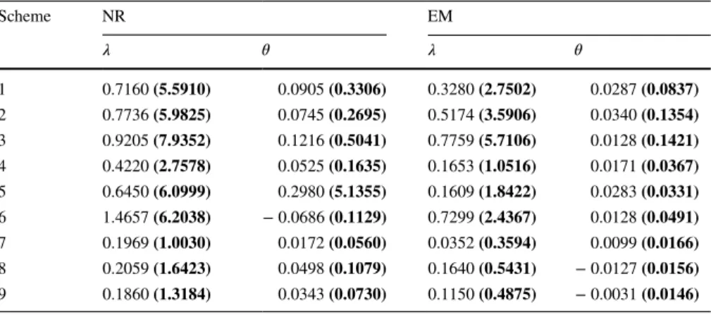
Table 3 Bias and MSE (in parentheses) of the estimators with 𝜆 = 5 and 𝜃 = 0.6
Scheme NR EM 𝜆 𝜃 𝜆 𝜃 1 0.7160 (5.5910) 0.0905 (0.3306) 0.3280 (2.7502) 0.0287 (0.0837) 2 0.7736 (5.9825) 0.0745 (0.2695) 0.5174 (3.5906) 0.0340 (0.1354) 3 0.9205 (7.9352) 0.1216 (0.5041) 0.7759 (5.7106) 0.0128 (0.1421) 4 0.4220 (2.7578) 0.0525 (0.1635) 0.1653 (1.0516) 0.0171 (0.0367) 5 0.6450 (6.0999) 0.2980 (5.1355) 0.1609 (1.8422) 0.0283 (0.0331) 6 1.4657 (6.2038) − 0.0686 (0.1129) 0.7299 (2.4367) 0.0128 (0.0491) 7 0.1969 (1.0030) 0.0172 (0.0560) 0.0352 (0.3594) 0.0099 (0.0166) 8 0.2059 (1.6423) 0.0498 (0.1079) 0.1640 (0.5431) − 0.0127 (0.0156) 9 0.1860 (1.3184) 0.0343 (0.0730) 0.1150 (0.4875) − 0.0031 (0.0146)
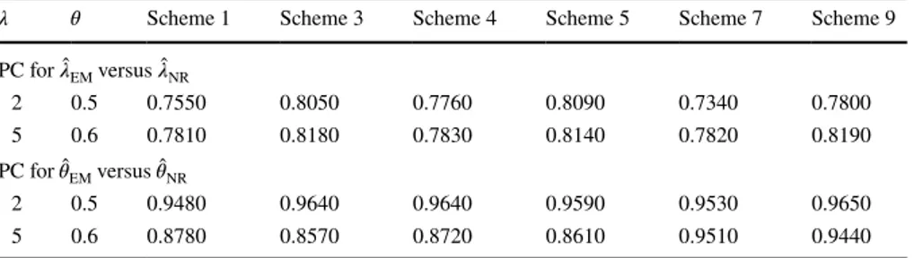
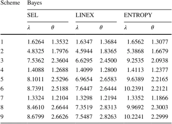
This simulation results reveal that the SEM is always superior to the NR method in terms of estimated biases, MSE’s. Further it is seen that SEM estimated is Pitman closer to the parameters than to the Bayes NR estimates. We also observe that the shrinkage Bayes estimated have smaller estimated risk than the usual Bayes esti-mated based on MCMC method. It is shown that the relative efficacies of the pro-posed shrinkage estimated are higher than 1 which is indicated to use of the shrink-ages estimators in the case of having suspected non-sample prior information. We also observe that the Bayes estimators based on M–H algorithm, mostly, perform those based on Lindely approximation and MCMC method.
4.1 Real Data Analysis
For illustrative purposes, here real data are analyzed using the proposed methods. A data set on the endurance of deep groove ball bearings analyzed by Lieblein and Zelen [23] consists of the number of million revolutions before failure for each of 23 ball bearings used in a life test. The data set is as follows.
Louzada et al. [26] indicated that the CEG can be fitted to this data set quite well. For our purpose, we generate three different schemes of progressive type-II censored sample as follows.
Scheme 1: R = (0, 0, 0, 0, 0, 0, 0, 0, 0, 0, 12) Scheme 2: R = (12, 0, 0, 0, 0, 0, 0, 0, 0, 0, 0) Scheme 3: R = (0, 0, 0, 0, 0, 0, 12, 0, 0, 0, 0)
The estimated values of the parameters are given in the following Tables 22, 23, 24 and 25 while the approximate and Bayesian confidence intervals are pre-sented in Table 26.
17.88 42.12 51.96 68.64 93.12 127.96 28.92 45.60 54.12 68.64 98.64 128.01 33.00 48.48 55.56 68.88 105.12 173.4 41.52 51.84 67.80 84.12 105.84
Table 4 PC comparison of MLEs based on EM and NR algorithms
𝜆 𝜃 Scheme 1 Scheme 3 Scheme 4 Scheme 5 Scheme 7 Scheme 9
PC for ̂𝜆EM versus ̂𝜆NR 2 0.5 0.7550 0.8050 0.7760 0.8090 0.7340 0.7800 5 0.6 0.7810 0.8180 0.7830 0.8140 0.7820 0.8190 PC for ̂𝜃EM versus ̂𝜃NR 2 0.5 0.9480 0.9640 0.9640 0.9590 0.9530 0.9650 5 0.6 0.8780 0.8570 0.8720 0.8610 0.9510 0.9440
Table
5
Bias and es
timated r
isk (in par
ent heses) of t he Ba yes es timat ors wit h 𝜆 = 2 and 𝜃 = 0 .5 Sc heme Ba yes SEL LINEX ENTR OPY 𝜆 𝜃 𝜆 𝜃 𝜆 𝜃 1 − 0.4328 (0.2669) 0.3185 (0.1046) − 0.4806 (0.1226) 0.3144 (0.0572) − 0.4956 (0.0525) 0.3087 (0.1394) 2 − 0.4457 (0.2914) 0.3188 (0.1048) − 0.4932 (0.1314) 0.3148 (0.0573) − 0.5081 (0.0571) 0.3090 (0.1396) 3 − 0.4910 (0.3331) 0.3231 (0.1074) − 0.5364 (0.1485) 0.3190 (0.0588) − 0.5524 (0.0657) 0.3133 (0.1428) 4 − 0.4721 (0.2764) 0.3812 (0.1468) − 0.4988 (0.1221) 0.3796 (0.0832) − 0.5075 (0.0501) 0.3776 (0.1937) 5 − 0.5771 (0.3767) 0.3849 (0.1495) − 0.6003 (0.1609) 0.3832 (0.0848) − 0.6103 (0.0694) 0.3811 (0.1966) 6 − 0.4537 (0.2613) 0.3817 (0.1471) − 0.4810 (0.1162) 0.3800 (0.0833) − 0.4895 (0.0471) 0.3780 (0.1940) 7 − 0.5178 (0.2914) 0.4411 (0.1950) − 0.5289 (0.1250) 0.4407 (0.1134) − 0.5329 (0.0486) 0.4403 (0.2493) 8 − 0.6005 (0.3799) 0.4424 (0.1961) − 0.6105 (0.1588) 0.4420 (0.1141) − 0.6149 (0.0648) 0.4416 (0.2505) 9 − 0.5718 (0.3498) 0.4419 (0.1957) − 0.5821 (0.1472) 0.4415 (0.1139) − 0.5863 (0.0593) 0.4411 (0.2500)
Table
6
Bias and es
timated r
isk (in par
ent heses) of t he Ba yes es timat ors wit h 𝜆 = 5 and 𝜃 = 0 .6 Sc heme Ba yes SEL LINEX ENTR OPY 𝜆 𝜃 𝜆 𝜃 𝜆 𝜃 1 − 1.2142 (1.8648) 0.2337 (0.0574) − 1.4947 (0.7565) 0.2294 (0.0302) − 1.3732 (0.0595) 0.2233 (0.0583) 2 − 1.2313 (1.9701) 0.2344 (0.0577) − 1.5118 (0.7756) 0.2301 (0.0304) − 1.3902 (0.0629) 0.2240 (0.0586) 3 − 1.3008 (2.1518) 0.2392 (0.0598) − 1.5764 (0.8278) 0.2350 (0.0316) − 1.4592 (0.0689) 0.2289 (0.0607) 4 − 1.1259 (1.5881) 0.2878 (0.0842) − 1.2987 (0.6149) 0.2860 (0.0460) − 1.2185 (0.0460) 0.2839 (0.0867) 5 − 1.3117 (1.9981) 0.2917 (0.0864) − 1.4700 (0.7318) 0.2900 (0.0473) − 1.4007 (0.0585) 0.2878 (0.0887) 6 − 1.0278 (1.3950) 0.2887 (0.0847) − 1.2103 (0.5587) 0.2870 (0.0463) − 1.1230 (0.0401) 0.2848 (0.0872) 7 − 1.0968 (1.3655) 0.3430 (0.1180) − 1.1744 (0.5091) 0.3426 (0.0663) − 1.1372 (0.0359) 0.3422 (0.1193) 8 − 1.2629 (1.7355) 0.3442 (0.1188) − 1.3350 (0.6170) 0.3438 (0.0668) − 1.3021 (0.0462) 0.3433 (0.1200) 9 − 1.1987 (1.6006) 0.3437 (0.1185) − 1.2726 (0.5763) 0.3433 (0.0666) − 1.2381 (0.0425) 0.3429 (0.1197)
5 Summary and Conclusion
In this paper, we proposed different estimators for the parameters of the comple-mentary exponential distribution. We obtained maximum likelihood estimators based on N–R and stochastic expectation maximization method as well. Further different sorts of Bayes estimates are obtained under various loss functions. We
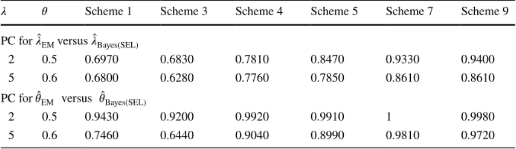
Table 7 PC comparison of MLEs based on EM and Bayes (under SEL function) algorithms
𝜆 𝜃 Scheme 1 Scheme 3 Scheme 4 Scheme 5 Scheme 7 Scheme 9
PC for ̂𝜆EM versus ̂𝜆Bayes(SEL)
2 0.5 0.6970 0.6830 0.7810 0.8470 0.9330 0.9400
5 0.6 0.6800 0.6280 0.7760 0.7850 0.8610 0.8610
PC for ̂𝜃EM versus ̂𝜃Bayes(SEL)
2 0.5 0.9430 0.9200 0.9920 0.9910 1 0.9980
5 0.6 0.7460 0.6440 0.9040 0.8990 0.9810 0.9720
Table 8 PC comparison of MLEs based on EM and Bayes (under LINEX loss function) algorithms
𝜆 𝜃 Scheme 1 Scheme 3 Scheme 4 Scheme 5 Scheme 7 Scheme 9
PC for ̂𝜆EM versus ̂𝜆Bayes(LINEX)
2 0.5 0.7210 0.6990 0.7990 0.8590 0.9370 0.9430
5 0.6 0.7460 0.6770 0.8160 0.8110 0.8830 0.8810
PC for ̂𝜃EM versus 𝜃̂Bayes(LINEX)
2 0.5 0.9420 0.9160 0.9920 0.9900 1 0.9980
5 0.6 0.7430 0.6350 0.9020 0.8980 0.9810 0.9720
Table 9 PC comparison of MLEs based on EM and Bayes (under ENTROPY loss function) algorithms
𝜆 𝜃 Scheme 1 Scheme 3 Scheme 4 Scheme 5 Scheme 7 Scheme 9
PC for ̂𝜆EM versus 𝜆̂Bayes(ENTROPY)
2 0.5 0.7280 0.7050 0.8010 0.8600 0.9370 0.9460
5 0.6 0.7160 0.6520 0.7980 0.7980 0.8710 0.8690
PC for ̂𝜃EM versus 𝜃̂Bayes(ENTROPY)
2 0.5 0.9390 0.9130 0.9910 0.9900 1 0.9980
Table
10
Bias and es
timated r
isk (in par
ent heses) of t he shr ink ag e es timat ors wit h 𝜆 = 2 and 𝜃 = 0 .5 Sc heme Ba yes SEL LINEX ENTR OPY 𝜆 𝜃 𝜆 𝜃 𝜆 𝜃 1 − 0.2829 (0.1641) 0.2696 (0.0773) − 0.3190 (0.0750) 0.2664 (0.0418) − 0.3302 (0.0317) 0.2619 (0.1066) 2 − 0.1459 (0.0603) 0.2350 (0.0583) − 0.1710 (0.0286) 0.2326 (0.0312) − 0.1790 (0.0106) 0.2290 (0.0837) 3 − 0.1455 (0.0442) 0.2115 (0.0455) − 0.1682 (0.0224) 0.2095 (0.0240) − 0.1762 (0.0071) 0.2066 (0.0682) 4 − 0.3527 (0.1962) 0.3322 (0.1157) − 0.3743 (0.0866) 0.3309 (0.0650) − 0.3815 (0.0355) 0.3292 (0.1565) 5 − 0.1885 (0.0465) 0.2424 (0.0591) − 0.2001 (0.0231) 0.2416 (0.0319) − 0.2051 (0.0072) 0.2406 (0.0887) 6 − 0.1269 (0.0299) 0.2408 (0.0584) − 0.1405 (0.0152) 0.2400 (0.0315) − 0.1448 (0.0046) 0.2390 (0.0877) 7 − 0.4120 (0.2187) 0.3937 (0.1611) − 0.4213 (0.0940) 0.3934 (0.0930) − 0.4247 (0.0364) 0.3930 (0.2101) 8 − 0.2002 (0.0449) 0.2712 (0.0736) − 0.2052 (0.0216) 0.2710 (0.0403) − 0.2074 (0.0065) 0.2708 (0.1089) 9 − 0.1859 (0.0403) 0.2709 (0.0735) − 0.1911 (0.0195) 0.2708 (0.0403) − 0.1932 (0.0058) 0.2706 (0.1087)
Table
11
Bias and es
timated r
isk (in par
ent heses) of t he shr ink ag e es timat ors wit h 𝜆 = 5 and 𝜃 = 0 .6 Sc heme Ba yes SEL LINEX ENTR OPY 𝜆 𝜃 𝜆 𝜃 𝜆 𝜃 1 − 0.8724 (1.1618) 0.2025 (0.0437) − 1.0842 (0.4846) 0.1992 (0.0228) − 0.9923 (0.0363) 0.1945 (0.0456) 2 − 0.5621 (0.5027) 0.1819 (0.0348) − 0.7108 (0.2364) 0.1792 (0.0181) − 0.6463 (0.0144) 0.1755 (0.0374) 3 − 0.5504 (0.4179) 0.1696 (0.0294) − 0.6882 (0.2130) 0.1675 (0.0152) − 0.6296 (0.0113) 0.1645 (0.0325) 4 − 0.8609 (1.0994) 0.2528 (0.0669) − 0.9995 (0.4318) 0.2514 (0.0363) − 0.9350 (0.0316) 0.2497 (0.0703) 5 − 0.5558 (0.3783) 0.1959 (0.0387) − 0.6350 (0.1815) 0.1950 (0.0205) − 0.6004 (0.0095) 0.1939 (0.0434) 6 − 0.4139 (0.2560) 0.1943 (0.0381) − 0.5051 (0.1311) 0.1935 (0.0202) − 0.4615 (0.0064) 0.1924 (0.0428) 7 − 0.8795 (0.9979) 0.3078 (0.0981) − 0.9434 (0.3780) 0.3075 (0.0548) − 0.9128 (0.0260) 0.3071 (0.1006) 8 − 0.5315 (0.3176) 0.2221 (0.0494) − 0.5675 (0.1440) 0.2219 (0.0266) − 0.5510 (0.0074) 0.2217 (0.0551) 9 − 0.4993 (0.2903) 0.2219 (0.0493) − 0.5363 (0.1327) 0.2217 (0.0266) − 0.5190 (0.0068) 0.2215 (0.0550)
also proposed the shrinkage estimators which has higher relative efficiency than the usual Bayes estimates. The Bayesian credible intervals are also computed by means of MCMC samples. We found that maximum likelihood estimators of the unknown parameters of the distribution do not admit closed form, and further the EM algo-rithm for this purpose still requires optimization technique to solve the involved expressions. Therefore, we considered the SEM algorithm to obtain the maximum likelihood estimators. In simulation study, we presented a comparison between the estimates obtained using SEM algorithm and estimates from Newton–Raphson and EM algorithm. We observed that the performance of SEM algorithm is quite sat-isfactory. For illustration purpose, we also considered a real data set. It should be mentioned here that the prediction of the future-order statistics based on the pro-gressive type-II censored samples is also in progress by the authors and we hope to report these results in another communication.
Table 12 Relative efficiencies (RE) of Bayesian shrinkage estimates with respect to the Bayes estimates with 𝜆 = 2 and
𝜃 = 0.5
Scheme Bayes
SEL LINEX ENTROPY
𝜆 𝜃 𝜆 𝜃 𝜆 𝜃 1 1.6264 1.3532 1.6347 1.3684 1.6562 1.3077 2 4.8325 1.7976 4.5944 1.8365 5.3868 1.6679 3 7.5362 2.3604 6.6295 2.4500 9.2535 2.0938 4 1.4088 1.2688 1.4099 1.2800 1.4113 1.2377 5 8.1011 2.5296 6.9654 2.6583 9.6389 2.2165 6 8.7391 2.5188 7.6447 2.6444 10.2391 2.2121 7 1.3324 1.2104 1.3298 1.2194 1.3352 1.1866 8 8.4610 2.6644 7.3519 2.8313 9.9692 2.3003 9 8.6799 2.6626 7.5487 2.8263 10.2241 2.2999
Table 13 Relative efficiencies (RE) of Bayesian shrinkage estimates with respect to the Bayes estimates with 𝜆 = 5 and
𝜃 = 0.6
Scheme Bayes
SEL LINEX ENTROPY
𝜆 𝜃 𝜆 𝜃 𝜆 𝜃 1 1.6051 1.3135 1.5611 1.3246 1.6391 1.2785 2 3.9190 1.6580 3.2809 1.6796 4.3681 1.5668 3 5.1491 2.0340 3.8864 2.0789 6.0973 1.8677 4 1.4445 1.2586 1.4240 1.2672 1.4557 1.2333 5 5.2818 2.2326 4.0320 2.3073 6.1579 2.0438 6 5.4492 2.2231 4.2616 2.2921 6.2656 2.0374 7 1.3684 1.2029 1.3468 1.2099 1.3808 1.1859 8 5.4644 2.4049 4.2847 2.5113 6.2432 2.1779 9 5.5136 2.4037 4.3429 2.5038 6.2500 2.1764
Table
14
Bias and es
timated r
isk (in par
ent heses) of t he Lindle y es timat ors wit h 𝜆 = 2 and 𝜃 = 0 .5 Sc heme Ba yes SEL LINEX ENTR OPY 𝜆 𝜃 𝜆 𝜃 𝜆 𝜃 1 0.9940 (1.4498) − 0.0237 (0.1788) 0.3522 (0.6861) − 0.0730 (0.1771) 0.6477 (1.2602) − 0.2068 (0.1709) 2 1.1899 (1.5371) − 0.0113 (0.1693) 0.4026 (0.7806) − 0.0653 (0.1728) 0.6427 (1.1852) − 0.2233 (0.1706) 3 0.8802 (1.0576) − 0.0686 (0.1220) 0.4282 (0.5463) − 0.0897 (0.1215) 0.6784 (1.1205) − 0.1474 (0.1223) 4 0.7657 (1.2828) − 0.0391 (0.1370) 0.2708 (0.5358) − 0.0738 (0.1425) 0.4862 (1.1282) − 0.1837 (0.1598) 5 0.1501 (0.0918) − 0.0123 (0.0316) 0.0755 (0.1099) − 0.0200 (0.0312) 0.0748 (0.1045) − 0.0400 (0.0278) 6 0.7007 (0.8937) − 0.0550 (0.1018) 0.4458 (0.5171) − 0.0724 (0.1066) 0.5752 (0.8559) − 0.1143 (0.1095) 7 0.5646 (1.2039) − 0.0351 (0.1126) 0.1959 (0.4489) − 0.0543 (0.1172) 0.3338 (0.8461) − 0.1371 (0.1539) 8 0.0607 (0.0312) − 0.0009 (0.0095) 0.0273 (0.0300) − 0.0051 (0.0101) 0.0273 (0.0300) − 0.0173 (0.0110) 9 0.0797 (0.0765) − 0.0052 (0.0325) 0.0438 (0.1071) − 0.0114 (0.0317) 0.0429 (0.0923) − 0.0283 (0.0284)
Table
15
Bias and es
timated r
isk (in par
ent heses) of t he Lindle y es timat ors wit h 𝜆 = 5 and 𝜃 = 0 .6 Sc heme Ba yes SEL LINEX ENTR OPY 𝜆 𝜃 𝜆 𝜃 𝜆 𝜃 1 1.4031 (1.1675) − 0.0550 (0.2314) − 0.1532 (0.8342) − 0.1029 (0.2055) 0.9165 (1.2086) − 0.2483 (0.2041) 2 1.6016 (1.1159) − 0.0455 (0.2172) − 0.2935 (0.7093) − 0.1197 (0.2128) 0.9875 (1.2077) − 0.2721 (0.1995) 3 2.0788 (1.0409) − 0.1015 (0.1665) 0.1033 (0.6786) − 0.1457 (0.1736) 1.4898 (1.1349) − 0.2348 (0.1707) 4 1.1925 (1.1882) − 0.0641 (0.1881) 0.0067 (0.7589) − 0.1108 (0.1864) 0.7850 (1.1195) − 0.2424 (0.2010) 5 0.4776 (0.3181) 0.0053 (0.0520) − 0.0976 (0.3247) − 0.0083 (0.0502) 0.2640 (0.3639) − 0.0387 (0.0512) 6 1.6841 (0.8989) − 0.0861 (0.1359) 0.4294 (0.6851) − 0.1124 (0.1414) 1.3957 (0.9901) − 0.1667 (0.1477) 7 0.7197 (0.9692) − 0.0555 (0.1399) 0.0458 (0.5179) − 0.0830 (0.1457) 0.4966 (0.9004) − 0.1826 (0.1899) 8 0.2313 (0.1225) − 0.0160 (0.0184) − 0.0120 (0.1227) − 0.0217 (0.0185) 0.1378 (0.1240) − 0.0339 (0.0178) 9 0.3581 (0.2922) − 0.0229 (0.0436) 0.0545 (0.2139) − 0.0317 (0.0443) 0.2423 (0.2288) − 0.0483 (0.0378)
Table
16
Bias and es
timated r
isk (in par
ent heses) of t he M–H algor ithm wit h 𝜆 = 2 and 𝜃 = 0 .5 Sc heme Ba yes SEL LINEX ENTR OPY 𝜆 𝜃 𝜆 𝜃 𝜆 𝜃 1 − 0.0477 (0.1608) 0.1046 (0.0248) − 0.1743 (0.0685) 0.0821 (0.0111) − 0.1814 (0.0231) 0.0069 (0.0488) 2 − 0.0381 (0.1603) 0.1032 (0.0236) − 0.1700 (0.0671) 0.0809 (0.0105) − 0.1770 (0.0229) 0.0073 (0.0434) 3 − 0.0655 (0.1837) 0.1058 (0.0236) − 0.2155 (0.0771) 0.0827 (0.0104) − 0.2246 (0.0269) 0.0053 (0.0460) 4 − 0.0420 (0.1430) 0.0941 (0.0262) − 0.1318 (0.0672) 0.0752 (0.0122) − 0.1342 (0.0186) 0.0169 (0.0483) 5 − 0.0822 (0.1474) 0.1131 (0.0267) − 0.2014 (0.0662) 0.0922 (0.0120) − 0.2070 (0.0217) 0.0270 (0.0435) 6 0.1179 (0.1607) 0.0688 (0.0196) − 0.0087 (0.0586) 0.0486 (0.0089) − 0.0047 (0.0146) − 0.0156 (0.0450) 7 − 0.0503 (0.0829) 0.0880 (0.0242) − 0.0995 (0.0409) 0.0743 (0.0115) − 0.1010 (0.0111) 0.0374 (0.0371) 8 − 0.0795 (0.0991) 0.0966 (0.0253) − 0.1443 (0.0473) 0.0813 (0.0119) − 0.1468 (0.0141) 0.0394 (0.0372) 9 − 0.0813 (0.0907) 0.0954 (0.0258) − 0.1383 (0.0442) 0.0813 (0.0123) − 0.1408 (0.0130) 0.0432 (0.0382)
Table
17
Bias and es
timated r
isk (in par
ent heses) of t he M–H algor ithm wit h 𝜆 = 5 and 𝜃 = 0 .6 Sc heme Ba yes SEL LINEX ENTR OPY 𝜆 𝜃 𝜆 𝜃 𝜆 𝜃 1 − 0.7501 (0.9834) 0.1145 (0.0187) − 1.2196 (0.5599) 0.0962 (0.0082) − 1.0058 (0.0346) 0.0449 (0.0166) 2 − 0.8009 (1.0855) 0.1224 (0.0200) − 1.2628 (0.5925) 0.1047 (0.0088) − 1.0553 (0.0382) 0.0564 (0.0159) 3 − 0.8767 (1.1527) 0.1377 (0.0226) − 1.3434 (0.6410) 0.1207 (0.0099) − 1.1417 (0.0421) 0.0756 (0.0156) 4 − 0.5544 (0.7147) 0.1168 (0.0212) − 0.9135 (0.3783) 0.1007 (0.0097) − 0.7337 (0.0216) 0.0591 (0.0200) 5 − 0.7575 (0.8880) 0.1462 (0.0256) − 1.1322 (0.4924) 0.1306 (0.0115) − 0.9592 (0.0294) 0.0915 (0.0194) 6 − 0.3128 (0.5196) 0.1070 (0.0192) − 0.7664 (0.2981) 0.0901 (0.0087) − 0.5355 (0.0150) 0.0455 (0.0197) 7 − 0.3541 (0.4632) 0.1116 (0.0238) − 0.5908 (0.2273) 0.0989 (0.0114) − 0.4620 (0.0118) 0.0693 (0.0249) 8 − 0.5193 (0.5588) 0.1298 (0.0253) − 0.7894 (0.2920) 0.1161 (0.0119) − 0.6497 (0.0157) 0.0843 (0.0233) 9 − 0.4453 (0.4872) 0.1132 (0.0222) − 0.7040 (0.2561) 0.1001 (0.0105) − 0.5673 (0.0133) 0.0700 (0.0215)
Table 18 Bayesian confidence
interval for 𝜆 = 2 and 𝜃 = 0.5 Scheme Bayesian confidence interval
𝜆 𝜃 1 (1.1056, 3.1061) (0.2190, 0.9667) 2 (1.1002, 3.1434) (0.2202, 0.9668) 3 (1.0457, 3.2321) (0.2155, 0.9695) 4 (1.2348, 2.8898) (0.2476, 0.9503) 5 (1.1365, 3.0676) (0.2406, 0.9648) 6 (1.2723, 3.2512) (0.2218, 0.9488) 7 (1.3942, 2.6143) (0.2999, 0.9160) 8 (1.3087, 2.6982) (0.2898, 0.9338) 9 (1.3325, 2.6418) (0.3013, 0.9255)
Table 19 Coverage probability (CP) of Bayesian confidence interval for 𝜆 = 2 and 𝜃 = 0.5
Scheme CP 𝜆 𝜃 1 0.9850 0.9940 2 0.9810 0.9950 3 0.9770 0.9960 4 0.9670 0.9840 5 0.9770 0.9960 6 0.9940 0.9970 7 0.9690 0.9770 8 0.9680 0.9860 9 0.9670 0.9690
Table 20 Bayesian confidence
interval for 𝜆 = 5 and 𝜃 = 0.6 Scheme Bayesian confidence interval
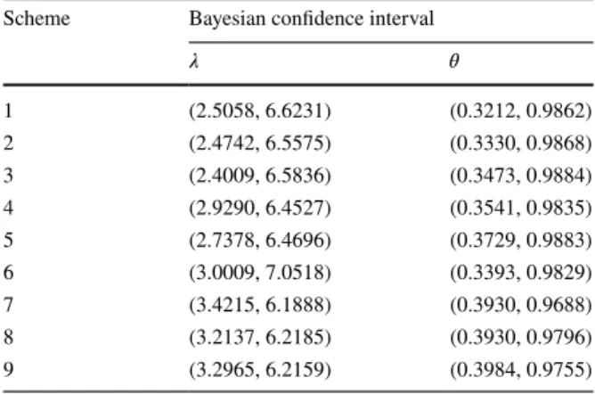
𝜆 𝜃 1 (2.5058, 6.6231) (0.3212, 0.9862) 2 (2.4742, 6.5575) (0.3330, 0.9868) 3 (2.4009, 6.5836) (0.3473, 0.9884) 4 (2.9290, 6.4527) (0.3541, 0.9835) 5 (2.7378, 6.4696) (0.3729, 0.9883) 6 (3.0009, 7.0518) (0.3393, 0.9829) 7 (3.4215, 6.1888) (0.3930, 0.9688) 8 (3.2137, 6.2185) (0.3930, 0.9796) 9 (3.2965, 6.2159) (0.3984, 0.9755)
Table 21 Coverage probability (CP) of Bayesian confidence interval for λ = 5 and 𝜃 = 0.6
Scheme CP 𝜆 𝜃 1 0.9630 1 2 0.9480 0.9990 3 0.9460 0.9990 4 0.9450 1 5 0.9470 1 6 0.9910 0.9980 7 0.9527 0.9776 8 0.9232 0.9875 9 0.9530 0.9780
Table 22 Estimated values of
λ and 𝜃 Scheme NR method SEM method
̂
𝜆 𝜃̂ 𝜆̂ 𝜃̂
1 0.09778 0.03752 0.04435 0.06966
2 0.06578 0.0185 0.04621 0.06537
3 0.07782 0.0105 0.06646 0.0182
Table 23 Estimated values of
λ and 𝜃 Scheme Bayes estimates (MCMC method)
SEL LINEX ENTROPY
̂
𝜆 𝜃̂ 𝜆̂ 𝜃̂ 𝜆̂ 𝜃̂
1 0.0128 0.6612 0.0128 0.64958 0.0121 0.6273 2 0.0143 0.6244 0.0143 0.6140 0.01375 0.6140 3 0.0118 0.6560 0.0118 0.6444 0.01125 0.6223
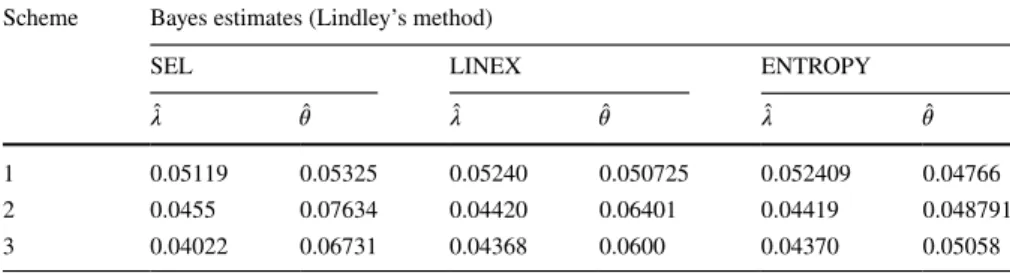
Table 24 Estimated values of λ and 𝜃
Scheme Bayes estimates (Lindley’s method)
SEL LINEX ENTROPY
̂
𝜆 𝜃̂ 𝜆̂ 𝜃̂ 𝜆̂ 𝜃̂
1 0.05119 0.05325 0.05240 0.050725 0.052409 0.04766
2 0.0455 0.07634 0.04420 0.06401 0.04419 0.048791
Acknowledgements This study was supported by the Scientific and Technological Research Council of Turkey (TUBITAK) and registered in 1059B211600192.
Appendix Lindley Method l𝜆𝜆= 𝜕2l 𝜕𝜆2 = − m 𝜆2 − 2 m ∑ i=1 𝜃(1 − 𝜃)x2 ie −𝜆xi [ e−𝜆xi(1 − 𝜃) + 𝜃]2 − m ∑ i=1 𝜃(1 − 𝜃)Rix2ie −𝜆xi [ e−𝜆xi(1 − 𝜃) + 𝜃]2 . l𝜃𝜃= 𝜕2l 𝜕𝜃2 = − m 𝜃2 + 2 m ∑ i=1 [ 1− e−𝜆xi]2 [ e−𝜆xi(1 − 𝜃) + 𝜃]2 − m ∑ i=1 Ri[1− e−𝜆xi]2 [ e−𝜆xi(1 − 𝜃) + 𝜃]2 . l𝜃𝜆= 𝜕 2l 𝜕𝜃𝜕𝜆 = l𝜆𝜃= 𝜕2l 𝜕𝜆𝜕𝜃 = −2 m ∑ i=1 ( xie−𝜆xi e−𝜆xi(1 − 𝜃) + 𝜃 + [ 1− e−𝜆xi]x ie−𝜆xi(1 − 𝜃) [ e−𝜆xi(1 − 𝜃) + 𝜃]2 ) − m ∑ i=1 ( Rixie−𝜆xi e−𝜆xi(1 − 𝜃) + 𝜃 + Ri [ 1− e−𝜆xi]x ie−𝜆xi(1 − 𝜃) [ e−𝜆xi(1 − 𝜃) + 𝜃]2 ) .
Table 25 Estimated values of
λ and 𝜃 Scheme Bayes estimates (M–H method)
SEL LINEX ENTROPY
̂
𝜆 𝜃̂ 𝜆̂ 𝜃̂ 𝜆̂ 𝜃̂
1 0.0700 0.0337 0.0698 0.0329 0.0630 0.0094 2 0.0293 0.2374 0.0293 0.2241 0.0258 0.1319 3 0.0248 0.2912 0.0247 0.2742 0.0209 0.2742
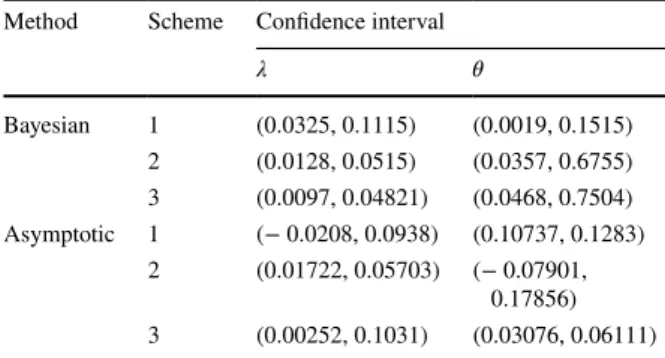
Table 26 Confidence interval
for λ and 𝜃 Method Scheme Confidence interval
λ 𝜃 Bayesian 1 (0.0325, 0.1115) (0.0019, 0.1515) 2 (0.0128, 0.0515) (0.0357, 0.6755) 3 (0.0097, 0.04821) (0.0468, 0.7504) Asymptotic 1 (− 0.0208, 0.0938) (0.10737, 0.1283) 2 (0.01722, 0.05703) (− 0.07901, 0.17856) 3 (0.00252, 0.1031) (0.03076, 0.06111)