Estimating soil texture with laser-guided Bouyoucos

2019, VOL. 61, NO. 1, 1–10

https://doi.org/10.1080/00051144.2019.1654283 REGULAR PAPER

Estimating soil texture with laser-guided Bouyoucos

Department of Computer Engineering, Cukurova University, Adana, Turkey

ABSTRACT

The main objective of estimating soil texture is to determine amounts of components of the soil. While the analysis of coarse particles is performed by sieving, Bouyoucos-hydrometer method is used to determine percentages of small particles (silt and clay, also sand). However, these tradi-tional methods require expertise, laboratory environment, sensitive equipment and a long-time period. All of these requirements are overcome by “Laser-Guided Bouyoucos” which is proposed in this study. The proposed device estimates the amount of components of soil by passing laser light through the beaker and evaluates the changes in the magnitude of light. Besides, the device requires no expert or laboratory medium for measurements, can be built using easy-to-find and cheap equipment, and most importantly, can be mobile for in-situ use. Several soil samples pre-analysed by Bouyoucos-hydrometer method are used in this study. The error of the proposed device was calculated by summing the absolute errors of sand, silt and clay components, and the average of all errors is only 2.25%. Although more soil samples are needed to test the sys-tem, according to the successful results on the used dataset, we believe that soil texture can be analysed quickly without an expert or a laboratory.

ARTICLE HISTORY Received 21 February 2019 Accepted 6 August 2019 KEYWORDS

Estimating soil texture; laser-guided Bouyoucos; LDR sensor; neural network; particle size

Introduction

Soil is an important material from which human beings have benefited since the beginning of the earth. Since the soil is a base component in some areas (agricultural activities for food production, constructional works for building shelters, and many others related to the mate-rial science), many issues in natural science such as drainage, water retention capacity, air capacity, erosion susceptibility, organic matter content, cation capacity, pH balance, hydraulic conductivity can be assessed with knowledge of the physical content of the soil [1–4]. By a simple definition, estimating soil texture is to measure the amount of sand, silt and clay particles [5]. While the amount of clay only can be used to comment the water retention capacity of the soil, the amount of organic nutrient waste for plants and the rate of mould, the amount of sand and silt together is used to determine whether the soil has sufficient air flow and whether or not it is suitable for agriculture. These three particle types are generally named according to their sizes in millimetres. Table 1 shows the classification of these components according to their particle sizes.

As shown in Table 1, particles between 2 and 0.02 mm are called “sand”, ones in [0.02 0.002] mm are “silt”, and particles smaller than 0.002 mm are “clay” [5]. Particles larger than 2 mm are not included in this classification. Particle types, particle distributions, basic principles underlying relations between particles, and methods to use in measuring are examined in a texture

analysis. Though hundreds of particle size determina-tion methods and proposals have been published to date [6], traditional and simple methods such as siev-ing, sedimentation, pipette and hydrometer methods are still considered to be the most commonly used standardized methods for estimation and measurement [5,7]. The classification of particle sizes mentioned above is based on Atterberg’s study. The mechanical analysis of the soil was first standardized in 1928 by the International Society of Soil Science as a combination of sieving and pipetting methods taking into consider-ation all the methods proposed so far and only particles passing through a 2 mm round pore sieve were taken into account.

The chemical structure of the particles also affects the physical content of the soil. For example, the dissolution of salts changes the particle size because the hydrolysis of the ions weakens the solidification between particles. Since soil and water come together in many of the problems related to the soil in the natural sciences, researchers often want to see also the water effect on the soil texture. Contrary to the ones with porous particles or a lot of organic mat-ter, mineral-bearing soil such as iron (haematite, fer-ric hydride, etc.), manganese (pyrolysis, benzene, etc.), titanium (ilmenite, titanomagnetite, etc.) is denser. Uti-lizing this density difference, if the prepared suspension is measured constantly at a certain depth and time intervals after mixing, some assessments can be made CONTACT Umut Orhan uorhan@cu.edu.tr Department of Computer Engineering, Cukurova University, 01330 Adana, Turkey

© 2019 The Author(s). Published by Informa UK Limited, trading as Taylor & Francis Group

This is an Open Access article distributed under the terms of the Creative Commons Attribution License (http://creativecommons.org/licenses/by/4.0/), which permits unrestricted use, distribution, and reproduction in any medium, provided the original work is properly cited.

Table 1.The classification of clay, silt and sand by the particle radius.

Radius (mm) Class Name

< 0.002 Clay

0.002–0.02 Silt

0.02–0.2 Fine sand

0.2–2.0 Coarse sand

about the materials above and below the Stokes’ diam-eter.

Many researchers classify the soil sample by consid-ering only particle types in higher ratio. The naming in this way facilitates general descriptions. For example, the texture analysis of clayey soils is more difficult than sandy ones. In addition to which particle type is in high amount, the size and the shape of the particles are the other important factors in classification. Since they can be represented by a single parameter in mathematical manner, all particles are tried to be expressed by spher-ical volume. Therefore, experts also classify particles according to whether they are spherical or not.

Since the traditional methods have some disadvan-tages such as causing high deviational results, requiring a lot of labour and experience, being dependent on equipment and laboratory, and having long duration, estimating soil texture is getting difficult [2,8]. For this reason, many studies on technology-supported analysis have been carried out [9–11].

Smart and Tovey [12] studied particles below 20 μm using electron microscopy. Additionally, optical meth-ods are frequently used in many areas such as colour analysis [13,14], plant root analysis [15,16], determina-tion of organic matter [17,18], soluble matter analysis [19,20], soil water interaction [21,22]. Chaney et al. [23] compared results of four different analysis devices (two devices are based on laser diffraction and other two uses X-Ray) with traditional hydrometer method. In Monson‘s study, a system consisting of two light sources producing light at different wavelengths and a camera was proposed to examine the physical struc-ture of agricultural land [24]. In another comparison study, Roberson and Weltje [25] used the sieve-pipette method and 10 particle size analyzer instrument for each sediment sample of Goossens [26] data. Fisher et al. [27] investigated the reliability of using the laser diffraction method to characterize the size of soil par-ticles. The results of a laser diffraction-based device and hydrometer method are evaluated in experiments using 22 soil samples collected from four different loca-tions. Sudarsan et al. [28] used the Continuous Wavelet Transform-based computer vision algorithm with a simple microscope connected to computer to charac-terize the size of soil particles. Frei and Kruis [29] used ANN (artificial neural network) both for regression and classification on transmission electron microscopy (TEM) images to analyse particle size distributions of agglomerates. Though successful results were obtained

by high-level technological equipment, such equipment has low potential in terms of price, availability, usage and portability.

By assessing all of these difficulties, a new device based on the traditional Bouyoucos experiment is improved. This device is designed by placing five laser light sources on one side of the beaker and five LDR (light dependent resistor) sensors on the other side, and it is fully automated with an embedded software. Although the soil preparation steps are the same with traditional Bouyoucos method, the device has some extra advantages as below.

• mobile and small

• work at any place (independence from laboratory) • self-work (independence from expert)

• cheap and easy producible.

Several soil samples which were preanalysed tradi-tionally are used to test the device. Final results are compared with Bouyoucos-hydrometer measurements.

Materials and methods

Soil samples and dataset preparation

Before starting the Bouyoucos-hydrometer method, 40 g of sodium hexametaphosphate is mixed with 1 L of purified water and allowed to fully dissolve for one day. Some amount of soil is taken from the dry soil sample (25 g for clayey soil, 50 g for loamy soil, and 100 g for sandy soil) and placed in an oven at about 105°C for 1 d. Then it is passed through a 2 mm sieve and elim-inated from big stones and its weight is measured. A new and same amount of soil sample is taken and mixed with the previously prepared 10 ml of sodium hexam-etaphosphate and 150 ml of distilled water solution, and left for 1 d. After mixing it in the dispersion vessel (5 min for sandy soil, 10 min for loamy soil, 15 min for clayey soil), the mixture is put into 1000 ml sedimen-tation cylinder (beaker) and distilled water is added up to 1000 ml line. The suspension is stirred thoroughly by moving it up and down 20 times with the brass mixing rod. Timer is started when the mixing rod is removed from the cylinder. After exactly 20 s, the hydrometer is gently immersed into the suspension and 40 s later the reading of the hydrometer is recorded. At the end of the 2nd hour of the experiment (again by immers-ing the hydrometer 20 s before), a second readimmers-ing is made. The temperature values are also recorded in both readings. If the temperature is different from 20°C the calculated ((ReadTemperature − 20) × 0.36) value is added to the recorded hydrometer value as a correc-tion. Both of the hydrometer readings are compared to the weight of the oven-dried soil sample. The ratio obtained from the first reading gives the percentage of “silt+ clay”, and the ratio obtained from the second

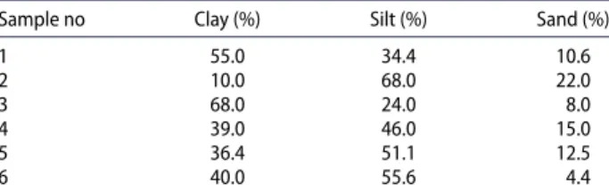
Table 2.Clay, silt and sand contents of soil samples used in the study.

Sample no Clay (%) Silt (%) Sand (%)

1 55.0 34.4 10.6 2 10.0 68.0 22.0 3 68.0 24.0 8.0 4 39.0 46.0 15.0 5 36.4 51.1 12.5 6 40.0 55.6 4.4

reading gives the percentage of “clay”. Sand, silt and clay percentages are determined using simple mathematical operations [7].

Six different soil samples were supplied from the Department of Geological Engineering of Çukurova University for using in the calibration and the test of the device proposed in this study. The clay, silt and sand percentages of the supplied soils were determined by the experts from three replicate experiments with conventional Bouyoucos-hydrometer analysis. In this study, the average of these three replicate experiments is used to calibrate the device. The contents of 6 soil sam-ples (averages of 3 replicate experiments) are given in Table2.

In the study, since they are difficult to determine, mostly silt and clay weighted soil samples were sup-plied. As seen in Table2, the contents of the samples vary from 4% to 22% sand, 24% to 68% silt and 10% to 68% clay. As a general opinion, it is argued that the sam-ple set should be formed by choosing from meaningful points that will represent the whole data. If the sample set is limited due to environmental conditions or dif-ficult to obtain subjects, the concept of “purposive” or “representativeness” emerges here. It is also possible for a small sample set to represent its parent population. In literature there are many statistical methods to evaluate whether a small sample set can be considered as reason-able or not [30]. In their work, using sample comple-tion rate and binomial distribucomple-tion, eight successfully evaluated sample out of nine have been considered as exceeding benchmark within the margin of 70%. In other words, with 80% probability 70% of the samples would complete the evaluation validly. This outcome claimed to be suitable for publication. Considering 6 out of 6 samples are successful in our dataset since the produced error rates (presented in “Results and Dis-cussion” section) are all lower than traditional Bouy-oucos error margin (5%), same calculation produces 61% completion rate. This indicates that by 76% proba-bility, 61% of the samples will be succeeded. Although it is barely sufficient evidence, promising results can drive us to overcome drawbacks due to small sample sizes in further researches.

Laser-guided Bouyoucos

In a preliminary work leading to this study, a simple system has been developed consisting of a LED (light

emitting diode) light source, nine LDR sensors and an embedded system to determine the sand percentage in a soil sample. Various mathematical methods have been applied to the data recorded in the measurements, and as a result, a proposal has been made that such a sys-tem can be used to determine the sand ratio in soil [31,32]. Although the mean squared error value about 1% level obtained in these studies was acceptable, the same success was not achieved for silt and clay rates.

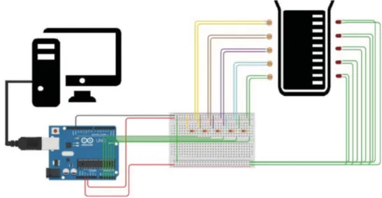
In the new system called Laser-Guided Bouyoucos (LGB), five homogenous red dot lasers instead of one LED and five LDR sensors are used. In the experi-ments, an Arduino microcomputer, a laptop computer, a beaker with 1000 ml, five homogeneous laser sources (flux density fixed at constant voltage) placed at one side of the beaker from bottom to top, and five LDR sen-sors at the other side of the beaker (each one facing to corresponding light source only) are used as shown in Figure1.

As seen in Figure1, the LGB is connected to a com-puter that gathers and interprets the data through an embedded circuit. The photographs of this experimen-tal setup, which is produced using simple, easy-to-find and cheap equipment, are shown in Figure2.

As seen in Figure2, the beaker can move without affecting other parts of the system. This prevents the dislocation of the sensors during agitation of soil-water suspension. The LGB is calibrated by placing the empty beaker in between lasers and LDR sensors in an iso-lated environment from any light. By this calibration made before each experiment, the magnitude of light reaching to the LDR sensors are used for normaliza-tion of min and max values. Then, adequately stirred soil-water suspension has been put into the beaker for each soil sample. After the pure water is added until the suspension level reaches 1000 ml line, the mixture is stirred by a long stirring rod until it has a homogeneous contexture. The experiments are carried out comply-ing with the same standards of Bouyoucos-hydrometer method (50 g soil preparation, sodium hexamethaphos-phate solution, fixed temperature at 20°C using digi-tal heating system, etc.). Lastly, the electronic system has been started for measurements. Figure 3 shows an overview of an experiment carried out in a dark environment.

As seen in Figure 3, the level of the bottom-most laser is considerably denser because of excessive par-ticle accumulation. Each LDR sensor measures a total of 90 min light intensity by taking 2 measurements in a second (2 Hz). Thus, a data with 5 rows (for each sen-sor) and 10,800 columns is obtained for a single exper-iment. The experiment is repeated one more time with a new instance of the same soil sample in order to elim-inate errors that can occur during measurement. After 2 repetitions for 90 min with 5 sensor data, as a result, data with 10 rows and 10,800 columns is obtained. This process is repeated all over again for 6 soil types, a data

Figure 1.Schematic representation of the experimental setup of the LGB.

Figure 2.The experimental setup (a) with beaker and (b) without beaker. set of 60 rows and 10,800 columns is created. For two

soil types, light intensity changes by time are shown in Figure4.

According to Figure4, the fastest illumination rate is observed in the 5th sensor at the top-most level of the beaker. On the other hand, while the illumination is considerably high about 1500th sampling for sensor #4 in Figure4(a), the same value is reached at 2500th sampling in sensor #4 of Figure4(b). We can roughly say that, the amount of sand in Figure 4(a) is more than the one in Figure4(b). However, when all of the sensor signals are plotted as shown in Figure5, it is inferred that the important moments of the conven-tional Bouyoucos method (40th second and 2nd hour) alone cannot provide meaningful information.

In Figure5, only the first 15 min of the signals are shown, so that the first 40 s looks better. According to the figure, almost no change has been observed at the top-most sensor (#5) up to 400th sampling (approx. 200 s). In the Bouyoucos analysis, however, the sand percentage can be determined by measuring only the first 40 s. This can be interpreted as that the laser light in the LGB system is blocked by small particles sus-pended in water and therefore did not reach to the LDR sensors, even at the top-most level of the beaker, for a long time (200 s). Nevertheless, this result shows that the estimation of the amount of sand can be possible by evaluating the whole of the signal. The data prepara-tion process of the LGB is given below in an algorithmic manner.

Figure 3.An overview of an experiment.

(1) Put the empty beaker in its place, and switch all lasers and LDR sensors on, check the light intensity values read by all LDRs. If they are not equiv-alent with a very small tolerance to each other, normalize it.

(2) Put the prepared soil and distilled water solution into the beaker, and fill the beaker up to 1000 ml line with distilled water and stir it adequately. (3) Start the electronic system, and store the values

measured at 2 Hz for 90 min by LDR sensors on the computer. At the end of each experiment, a dataset with 5 rows (one for each sensor) and 10,800 columns (2 Hz× 90 min × 60 s) is obtained. (4) Drain and clean the beaker after each experiment.

Make two repetitions for each experiment of each soil sample.

(5) If there is an untried soil sample, go to step 1 for this sample.

(6) As a result, a dataset with 60 rows and 10,800 columns is generated.

It is necessary to extract some meaningful features from the dataset obtained as the result of the data prepa-ration process before giving it as input to the prediction system. In this phase, some features of each row in the dataset are extracted by using most common used statistical functions in the literature such as standard deviation, entropy, mean, min and max. Because of the results found in the previous study [32], standard

Figure 4.Plots of light intensity by the time of (a) soil type #2 and (b) soil type #6.

Figure 6.Structure of a multi-layer neural network.

deviation and entropy functions are chosen to extract features. Thus, the dataset is transformed into a new format with 60 rows and 2 columns. Then, a com-puterized prediction process is started by using this dataset.

For doing computational prediction, ANN models are the best-known methods in the literature. ANN models are designed to imitate the ability of the human brain generating logical responses to new situations by using previous experiences [33]. ANNs are used in many areas such as prediction, classification, identifica-tion, generalizaidentifica-tion, association. ANNs have the ability to learn and deduct themselves by keeping the sam-ple situations they meet. The mathematical working principle of ANN is based on the update of randomly determined weight values at the beginning. When they are properly trained, they can produce decent results even with incomplete data (Figure6).

The multilayered perceptron (MLP) is not only the most preferred ANN model, and at the same time it is a basis system for almost all of the deep learning tools that are popular today.

Results and discussion

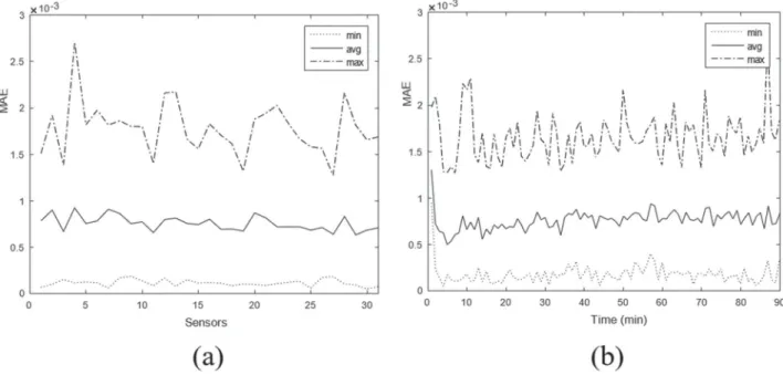
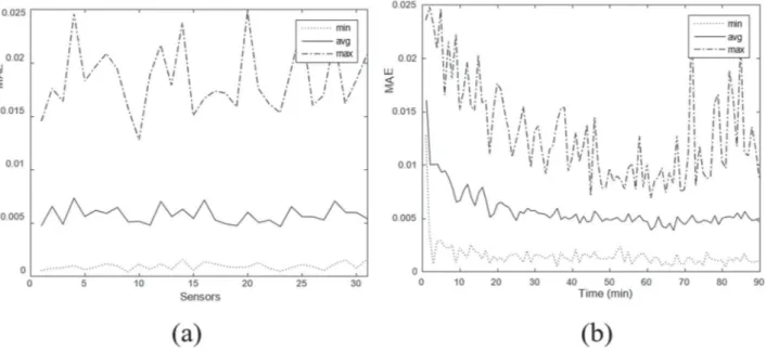
In the LGB system, a traditional MLP structure with three layers (input, hidden, and output) is used. There are 10 neurons in the single hidden layer, and activa-tion funcactiva-tion is hyperbolic tangent for all neurons. For the validation, 6-fold cross-validation method has been applied. Data of 5 soil samples are used to train the MLP system, while the data of remaining 1 soil sample is used as test data to measure the success. This procedure is repeated a total of 6 times as each soil sample is to be test data once. The average of all test results is determined as the overall system performance. Since the MLP here tries to predict the amount of sand, silt, and clay by using two extracted features (standard deviation and entropy) from LDR sensor signals, the error of the sys-tem is calculated as the success according to law of low error for high success. Among many types of errors, the mean absolute error (MAE) is chosen for this study, and the differences between the expected value and the obtained value are summed for each soil component. As a summary, the LGB system measures signals by five LDR sensors, then extracts two features for each sig-nal, and lastly gives these features to the MLP predictor. In order to decrease the size of input signals, at first, a study was made on which sensor combinations and how short the measurement duration can give the most successful result. Because of the five sensors, there are 31 (25 − 1) different sensors combinations. The MAE values obtained from the first 90 min segment for dif-ferent time lengths of the measurement data and for the different sensor combinations for estimating amount of sand are shown in Figure7, and the ones for estimating amount of silt are shown in Figure8.

For both Figures7(a) and 8(a), each sensor combi-nation represents the decimal value of sensors used in binary form for that experiment, in other word, 5 means

Figure 8.The MAE (mean absolute error) values (a) by sensor combinations, and (b) by time lengths for silt determination. “00101” and 25 means “11001” sensor combinations,

as illustrated in Figure9as well. For both Figures7(b) and 8(b), each time value starts from the beginning of that experiment, in other word, 10 means [0 10] and 20 means [0 20] minutes’ time intervals. In Figure7, both images show the minimum, the average, and the maxi-mum of the obtained errors (min–avg–max among dif-ferent sensor combinations for 7.a and min–avg–max among different time lengths for 7.b). According to Figure7, although the lowest error is occurred at 4th minute with the 0.004% MAE, the 0.05% MAE value on the “average” curve at 5th minute is considered as a consistent result. Accordingly, it has been determined that a 5-min measurement is enough to detect sand in the soil samples used in the study. A similar approach has been performed for sensor combinations that pro-duce the best results on the average curve. Accordingly, the four closest combinations starting from the low-est MAE value were 29th (11101), 27th (11011), 11th (01011) and 3rd (00011). Based on their binary repre-sentations, it has been determined that the most valu-able one among five sensors is the top-most LDR sensor in the device (the last bit in the four combinations), and the most successful combination is all the sensors together except the second sensor from the top (29th combination).

Figure8shows that although the overall image looks bad compared to the sand test, the silt estimates are also promising. Since the minimum MAE was reached at 81st minute, it can be said that approximately 81 min of measurement is sufficient to determine the silt per-centage. Although reasonable MAE values have been encountered earlier than 81st minute, it can only be said definitely after being sure there is no more MAE drop off for the remaining plot. It also turns out that the most significant sensor is the top-most sensor, and the best sensors to detect the silt percentage are the second and

Figure 9.Decimal representation of combination of LEDs using binary. (e.g. Combination 25 means taking 1st, 2nd and 5th LDR sensors’ data from bottom to top into calculations like they are on, and excluding data of 3rdand 4th LDRs like they are off. Dec-imal representation of the combination above: 11001= 25).

third sensors from the top. When the system detects sand and silt ratios in detail, then clay amount can be calculated by using 1− (sand + silt).

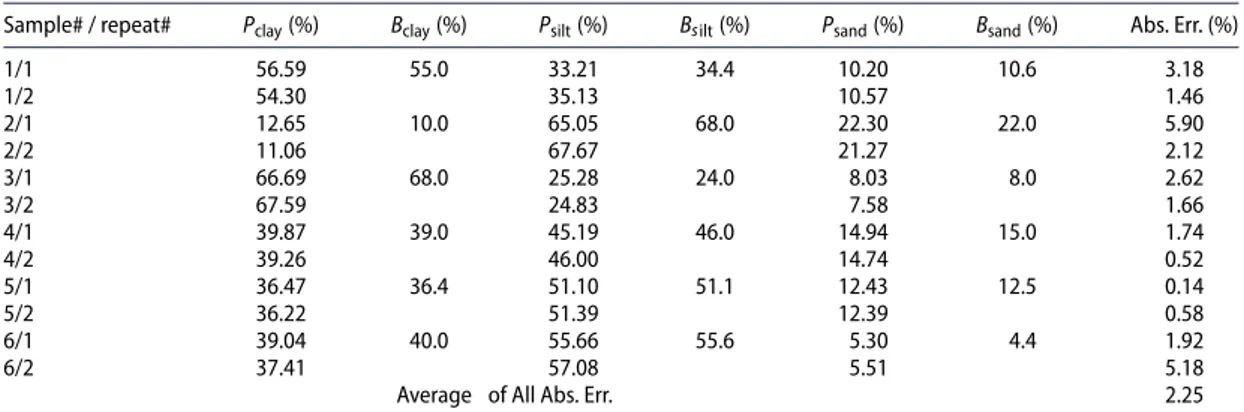
In order to show the success of the proposed sys-tem, an application is performed on the soil samples in Table2. The best sensor combinations described above (the top-most sensor only for sand, the second and third sensors together for silt) and the shortest possible durations (5 min for sand and 81 min for silt) restricted the signals, then the features are extracted, and all data have been given to the MLP model (two experiments done with the same soil sample used for test and the remaining ones for train). The obtained estimations are presented in Table3.

In Table3, the contents of each soil sample (sand, silt, clay) used in the experiments are given in two different

Table 3.Clay, silt and sand percentages detected by the LGB and Bouyoucos.

Sample# / repeat# _Pclay(%) Bclay(%) Psilt(%) Bsilt(%) Psand(%) Bsand(%) Abs. Err. (%)

1/1 56.59 55.0 33.21 34.4 10.20 10.6 3.18 1/2 54.30 35.13 10.57 1.46 2/1 12.65 10.0 65.05 68.0 22.30 22.0 5.90 2/2 11.06 67.67 21.27 2.12 3/1 66.69 68.0 25.28 24.0 8.03 8.0 2.62 3/2 67.59 24.83 7.58 1.66 4/1 39.87 39.0 45.19 46.0 14.94 15.0 1.74 4/2 39.26 46.00 14.74 0.52 5/1 36.47 36.4 51.10 51.1 12.43 12.5 0.14 5/2 36.22 51.39 12.39 0.58 6/1 39.04 40.0 55.66 55.6 5.30 4.4 1.92 6/2 37.41 57.08 5.51 5.18

Average of All Abs. Err. 2.25

Note: P notation stands for predicted result using proposed LGB method, B notation stands for Bouyoucos results obtained in laboratory medium. Abs. Err is the error between the predicted result and the actual Bouyoucos result.

Figure 10.TheR2values for (a) clay, (b) silt, (c) sand.

columns for a better comparison. “Psand(%)” represents the sand amount predicted by the LGB and “Bsand(%)” is the sand amount obtained by the Bouyoucos analysis. According to the table, if the Bouyoucos-hydrometer method and the LGB are compared, it is observed that the maximum absolute error (Abs. Err.) occurred in the first experiment of soil sample #2 with 5.90%, and the average of all Abs. Err. values is 2.25%. It can be said that very successful results are obtained since ±5% devi-ation is acceptable even in the traditional Bouyoucos experiment. On the other side,R2values are given in Figure10for each soil component.

As seen in Figure 10, R2 values are greater than 0.99. In the literature, there are some studies used R2 as success measurements, in which the results can be compared to each other. According to the Roberson and Weltje[25], laser diffraction-based devices (Fritsch Analysette 22C and Horiba Partica LA-950) outper-formed the sediment based systems with the 0.96 and 0.97 for R2 values, respectively. The approach used in [28] reached 0.87 for coarse fractions and 0.88 for fine fractions as the best R2 results. Fisher et al. [27] proposed different thresholds (< 9, < 26, and < 275 μm) for Particle Size Distribution in Laser Diffraction Methods which corresponds < 2, < 20, and < 200 μm thresholds in Bouyoucos-hydrometer

method, respectively. But Lin’s concordance correla-tion coefficient used instead of R2 are only found as 0.82, 0.97 and 0.88 with respect to < 9, < 26, and < 275 μm thresholds. Although only a few soil samples are tested in our study, the results proved that the LGB system is a good idea to work on when considering the literature studies. It is clear that more experiments are required to ensure the reliability of the system. In addi-tion, there are some concerns for clayey soils because of the reasons such as the reflection of light and the inabil-ity of rays to reach the LDR sensors on the opposite side of the beaker for a long time.

Conclusion

Conventional analysis methods such as the Bouyoucos-hydrometer method are still used in the physical anal-ysis of soils in fields requiring soil treatment such as agriculture, construction and mining. These methods are both laborious and time consuming as much as they are successful and reliable. It is a great disadvantage that analysis requires both an expert and a long time. Considering today’s technology, this study has been carried out to demonstrate that soil texture can be anal-ysed more effectively by utilizing the speed, power and success of computerized systems. Thus, a new device

can be produced, which is easy-to-use, fast resulting, independent from the expert, with high accuracy and consistency.

In this study, a device called the LGB, which is based on five sensor-pairs and a simple embedded electronic system was designed to determine the percentage of sand, silt and clay in the soil. Because the light cannot reach the LDR sensors for a long time due to the clay component, the sand ratio estimated at 40 s in Bouy-oucos experiments could not be estimated before of 5 min in this study. But the whole process is short-ened. When the LGB is compared with the Bouyoucos-hydrometer method, the results of the LGB system are almost identical to those of the Bouyoucos method. Although the system needs to be tested with far more soil samples, the high success achieved is noteworthy. Furthermore, the modular design of the device allows for possible improvements. Thus, hardware revisions can be easily done to remove concerns about clayey soils with future works.

Disclosure statement

No potential conflict of interest was reported by the authors.

ORCID

Umut Orhan http://orcid.org/0000-0003-1882-6567

Emre Kılınç http://orcid.org/0000-0002-5250-9322

References

[1] Florian S, Zaucă DC, Pavel LV. Soil structure and water-stable aggregates. Environ Eng Manag J. 2013;12(4): 741–746.DOI:10.30638/eemj.2013.091.

[2] Kettler T, Doran JW, Gilbert TL. Simplified method for soil particle-size determination to accompany soil-quality analyses. Soil Sci. Soc. Am. J.2001;65:849–852.

DOI:10.2136/sssaj2001.653849x.

[3] Saxton KE, Rawls WJ. Soil water characteristic esti-mates by texture and organic matter for hydro-logic solutions. Soil Sci Soc Am J. 2006;70(5):1569.

DOI:10.2136/sssaj2005.0117.

[4] Sedaghat A, Bayat H, Safari Sinegani AA. Estimation of soil saturated hydraulic conductivity by artificial neural networks ensemble in smectitic soils. Eurasian Soil Sci-ence. 2016;49(3):347–357. DOI:10.1134/S1064229316

03008X.

[5] Gee GW, Bauder JW. Particle size analysis. In: Klute A, editor. Methods of soil analysis. Part 1. Physical and mineralogical methods. Madison: Agronomy Mono-graphs, ASA and SSSA;1986. p. 388–411.DOI:10.2136/

sssabookser5.1.2ed.c15.

[6] Syvitski JPM. (1991). Principles, methods, and appli-cation of particle size analysis. In J. P. M. Syvit-ski, editor. Cambridge: Cambridge University Press. DOI:10.1017/CBO9780511626142.

[7] Bouyoucos GJ. Hydrometer method improved for making particle size analysis of soil. Soc Agro J.

1962;54:465–466.

[8] Centeri C, Jakab G, Szabo S, et al. Comparison of particle-size analyzing laboratory methods. Environ Eng Manag J.2015;14:1125–1135.

[9] Barak P, Mcsweeney K, Seybold CA. Self-similitude and fractal dimension of sand grains. Soil Sci Soc Am J – SSSAJ. 1996;60. DOI:10.2136/sssaj1996.036159950060 00010013x

[10] Grout H, Tarquis AM, Wiesner MR. Multifractal analy-sis of particle size distributions in soil. Environ Sci Tech-nol.1998;32(9):1176–1182.DOI 10.1021/es9704343. [11] Tyler SW, Wheatcraft SW. Fractal scaling of soil

particle-size distributions: analysis and limitations. Soil Sci Soc Am J.1992;56(2):362.DOI:10.2136/sssaj1992.0361599

5005600020005x.

[12] Smart P, Tovey NK. Electron microscopy of soils and sediments: techniques. Oxford: Clarendon Press;1982. [13] Czachor H, Lipiec J. Quantification of soil

macroporos-ity with image analysis**. Int Agrophysics.2004;18(3): 217–223. Available from:https://www.researchgate.net/ publication/26551726_Quantification_of_soil_macro

porosity_with_image_analysis.

[14] Stiglitz R, Mikhailova E, Post C, et al. Evaluation of an inexpensive sensor to measure soil color. Comput Elec-tron Agric.2016;121:141–148.DOI:10.1016/j.compag.

2015.11.014.

[15] Galkovskyi T, Mileyko Y, Bucksch A, et al. Gia roots: software for the high throughput analysis of plant root system architecture. BMC Plant Biol.2012;12(1):116.

DOI:10.1186/1471-2229-12-116.

[16] Kimura K, Kikuchi S, Yamasaki S. Accurate root length measurement by image analysis. Plant Soil.1999; 216(1–2):117–127.DOI:10.1023/A:1004778925316. [17] Chen Y, Katan J, Gamliel A, et al. Involvement of

soluble organic matter in increased plant growth in solarized soils. Biol Fertil Soils. 2000;32(1):28–34.

DOI:10.1007/s003740000209.

[18] Hummel JW, Sudduth KA, Hollinger SE. Soil moisture and organic matter prediction of surface and subsurface soils using an NIR soil sensor. Comput Electron Agric.

2001;32(2):149–165. DOI:10.1016/S0168-1699(01)

00163-6.

[19] Forrer I, Papritz A, Kasteel R, et al. Quantifying dye trac-ers in soil profiles by image processing. Eur J Soil Sci.

2000;51(2):313–322. DOI:10.1046/j.1365-2389.2000.

00315.x.

[20] Qing Z, Ji B, Zude M. Predicting soluble solid con-tent and firmness in apple fruit by means of laser light backscattering image analysis. J Food Eng.2007;82(1): 58–67.DOI:10.1016/j.jfoodeng.2007.01.016.

[21] Persson M. Estimating Surface soil Moisture from soil color using image analysis. Vadose zone J. 2005;4.

DOI:10.2136/vzj2005.0023.

[22] Santos JFCd, Silva HRF, Pinto FAC, et al. Use of digi-tal images to estimate soil moisture. Revista Brasileira Engenharia Agríc Ambiental. 2016;20:1051–1056. Available from: http://www.scielo.br/scielo.php?script = sci_arttext&pid = S1415-43662016001201051&nrm

= iso.

[23] Chaney R, Demars K, Vitton S, et al. Particle-size analysis of soils using laser light scattering and X-ray absorption technology. Geotech Test J.1997;20(1):63.

DOI:10.1520/GTJ11421J.

[24] Monson RJ. (2003). Soil particle and soil analysis sys-tem. Available from:https://patents.google.com/patent/

US6570999B1/en.

[25] Roberson S, Weltje GJ. Inter-instrument comparison of particle-size analysers. Sedimentology. 2014;61(4): 1157–1174.DOI:10.1111/sed.12093.

[26] Goossens D. Techniques to measure grain-size distri-butions of loamy sediments: a comparative study of

ten instruments for wet analysis. Sedimentology.2007; 55(1):65–96.DOI:10.1111/j.1365-3091.2007.00893.x. [27] Fisher P, Aumann C, Chia K, et al. Adequacy of laser

diffraction for soil particle size analysis. PLOS ONE.

2017;12(5):e0176510. DOI:10.1371/journal.pone.

0176510.

[28] Sudarsan B, Ji W, Adamchuk V, et al. Characterizing soil particle sizes using wavelet analysis of microscope images. Comput Electron Agric. 2018;148(March): 217–225.DOI:10.1016/j.compag.2018.03.019.

[29] Frei M, Kruis FE. Fully automated primary particle size analysis of agglomerates on transmission electron microscopy images via artificial neural networks. Pow-der Technol. 2018;332:120–130. DOI:10.1016/J.POW

TEC.2018.03.032.

[30] Sauro J, Lewis JR. (2016). Quantifying the user experi-ence (second edition). In: Quantifying the user expe-rience (pp. 9–18). DOI:10.1016/B978-0-12-802308-2.

00002-3.

[31] Gök H, Orhan U. (2015). Topraktaki Kum Oranının Bilgisayar Destekli Tespiti. 23. Sinyal İşleme ve İletişim Uygulamaları Kurultayı; Adana. p. 1178–1181. [32] Kılınç E, Orhan U. (2016). Estimation of sand ratio

in soil by LDR sensors and linear regression. 1st International Mediterranean Science and Engineering Congress; Adana p. 1335–1342.

[33] Hill T, Marquez L, O’Connor M, et al. Artificial neu-ral network models for forecasting and decision mak-ing. Int J Forecast.1994;10(1):5–15.