Short-term solar irradiance forecasting with deep neural networks

(1)

KADİR HAS UNIVERSITY SCHOOL OF GRADUATE STUDIES

PROGRAM OF MANAGEMENT INFORMATION SYSTEMS

SHORT-TERM SOLAR IRRADIANCE FORECASTING

WITH DEEP NEURAL NETWORKS

CANER VATANSEVER

MASTER’S THESIS

(2)

Caner Vatansever M.S. Thesis 201 9 S tude nt ’s F ul l N am e P h.D . (or M .S . or M .A .) T he si s 20 11

(3)

SHORT-TERM SOLAR IRRADIANCE FORECASTING

WITH DEEP NEURAL NETWORKS

CANER VATANSEVER

MASTER’S THESIS

Submitted to the School of Graduate Studies of Kadir Has University in partial fulfillment of the requirements for the degree of Master’s in the Program of

Management Information Systems

(4)

(5)

(6)

ABSTRACT

Usage of solar energy has increased through the last decades, and they are being in-tegrated into main grid systems since the recent years. In order to fully benefit from solar panels, predicting irradiance is essential. By knowing 15-minute ahead values of solar irradiance, resistance of the cells inside the solar panels can be measured to analyze production output. This study focuses on 15-minute ahead forecasting of irradiance by using sliding windows method on the feature set. ANN, K-NN, SVM and RF models are optimized in this study. As the result of the study, around 6% MAPE is achieved.

Keywords: Solar Irradiance Forecasting, Artificial Neural Networks, Ran-dom Forest, K-Nearest Neighbor, Short Term Forecasting

(8)

DER˙IN S˙IN˙IR A ˘GLARI KULLANIMIYLA KISA S ¨UREL˙I G ¨UNES¸ IS¸IMASI TAHM˙INLEMES˙I

¨

OZET

Güne¸s enerjisinin kullanımı son 10 yıl i¸cerisinde art¸s göstermektedir. Ek olarak bu kullanım, son yıllarda, ¸sebeke sistemleri ile entegre edilmeye ba¸slanm¸stır. Güne¸s panellerinden tamamıyla yararlanabilmek i¸cin, ı¸sımayı tahmin edebilmek ¸cok önemlidir. 15 dakika sonrasındaki güne¸s ı¸sıması de˘gerlerini bilerek, güne¸s paneli i¸cerisindeki direnci tahmin edebilir ve üretimi analiz edebiliriz. Bu ¸calı¸sma sürgülü pencere yöntemini kullanarak 15 dakika sonrasındaki ı¸sıma tahminlemesine odaklanmı¸stır. Yapay sinir a˘gları, k-en yakın kom¸su ve rassal orman modelleri bu ¸calı¸smada opti-mize edilmi¸stir. Bu ¸calı¸smanın sonucunda, yakla¸sık olarak 6% mutlak yüzde hataya ula¸sılmı¸stır

Anahtar Sözcükler: Güne¸s I¸sıma Tahminlemesi, Yapay Sinir A˘gları, Ras-sal Orman, K-En Yakın Kom¸su, Kısa Dönemli Tahminleme

(9)

ACKNOWLEDGEMENTS

I would like to express my deep gratitude to Professor Hasan Da˘g and Dr. O˘guzhan Ceylan, my research supervisors, for their patient guidance, enthusiastic encour-agement and useful critiques of this research work. I would also like to thank Dr. O˘guzhan Ceylan, for her advice and assistance in keeping my progress on schedule. My grateful thanks are also extended to Mr. Yunus Kolo˘glu for his help in doing the raw data analysis.

Nobody has been more important to me in the pursuit of this project than the members of my family. I would like to thank my parents, whose love and guidance are with me in whatever I pursue. They are the ultimate role models. Most importantly, I wish to thank my loving and supportive wife, Semanur, and my little wonderful daughter, Yaren, who provide unending inspiration.

(10)

(11)

LIST OF TABLES

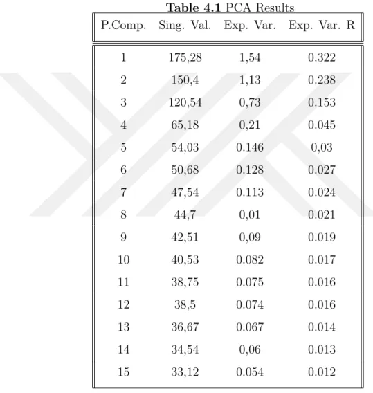
Table 4.1 PCA Results . . . 40

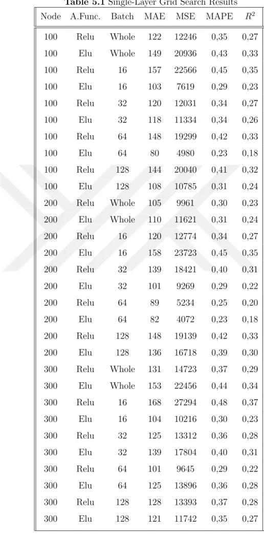
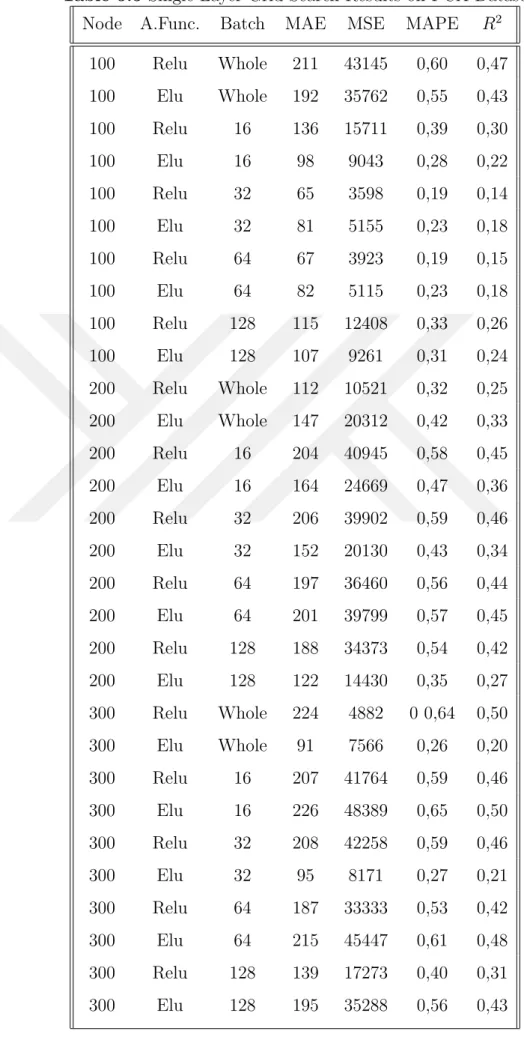
Table 5.1 Single-Layer Grid Search Results . . . 42

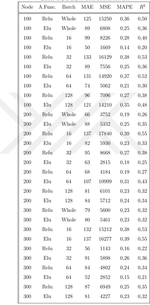
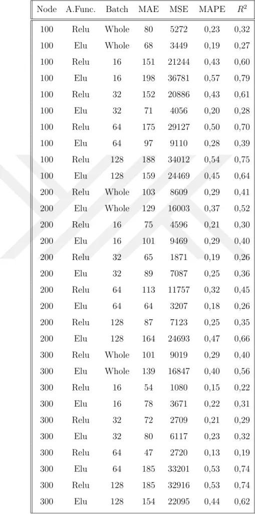
Table 5.2 2-Layer Grid Search Results . . . 43

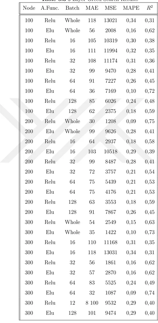
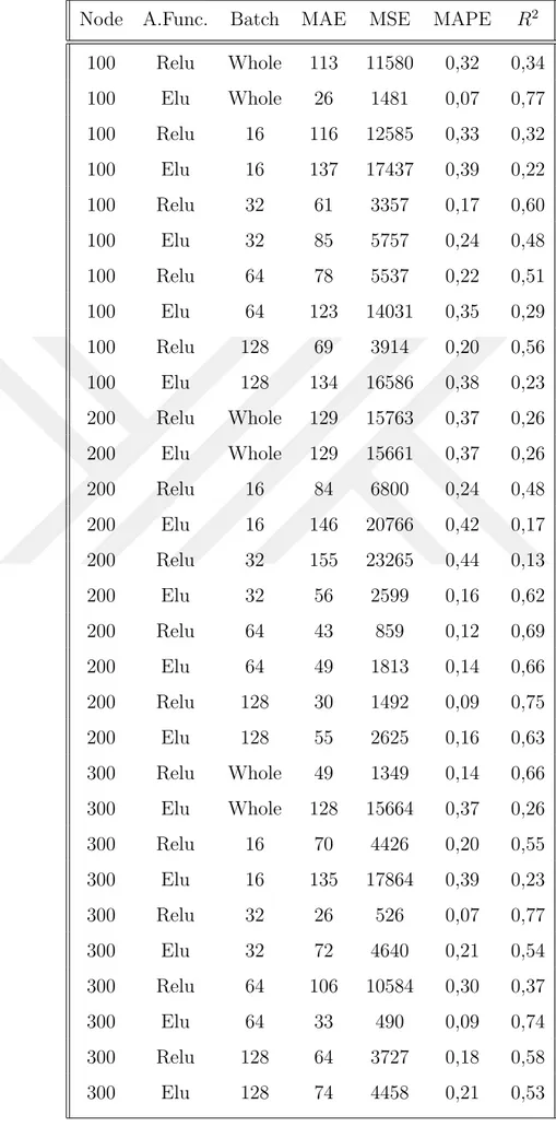
Table 5.3 3-Layer Greed Search Results . . . 44

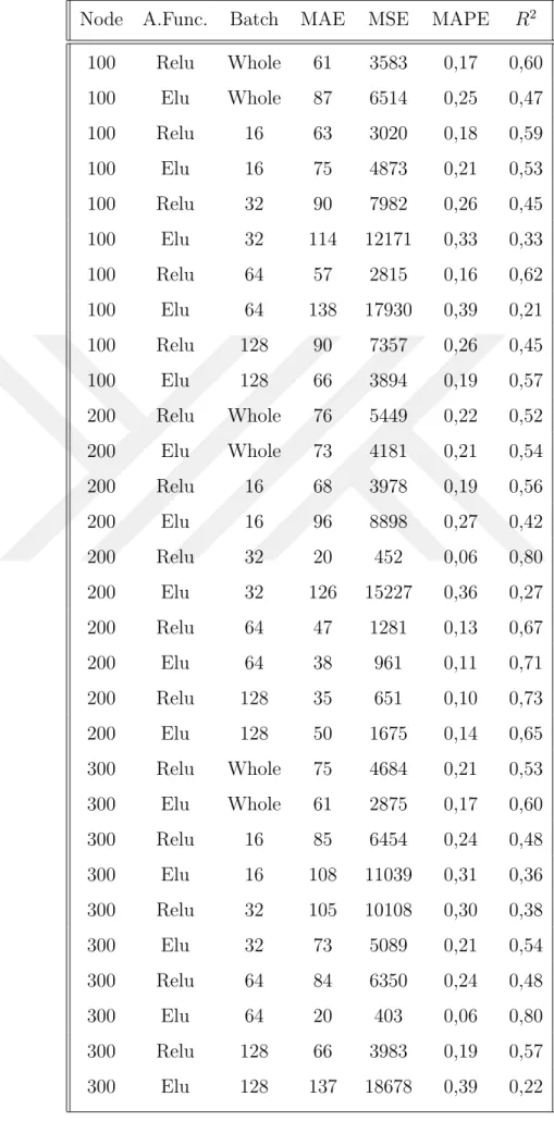
Table 5.4 4-Layer Grid Search Results . . . 45

Table 5.5 Single Layer Grid Search Results on PCA Dataset . . . 47

Table 5.6 2-Layer Grid Search Results on PCA Dataset . . . 48

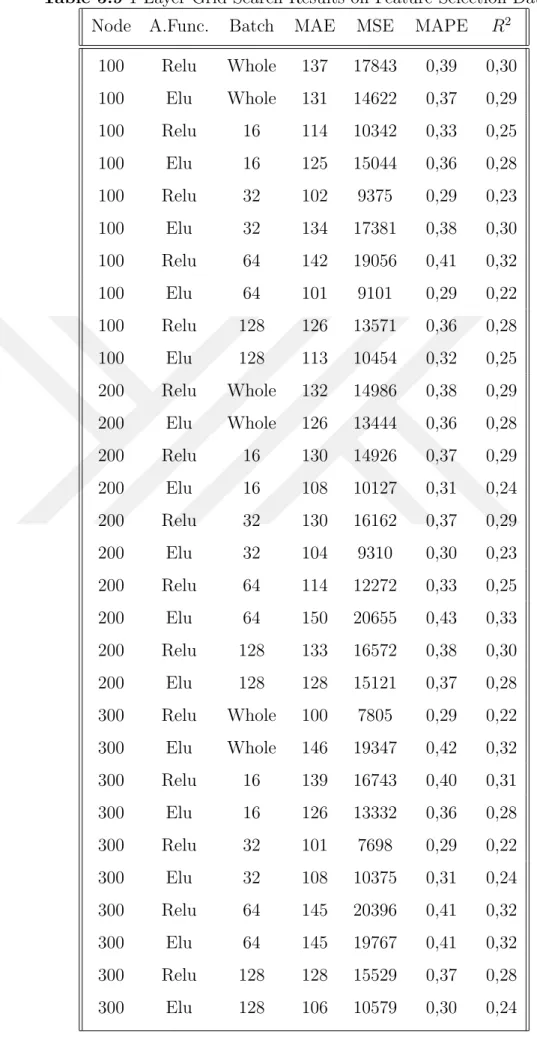
Table 5.9 1-Layer Grid Search Results on Feature Selection Dataset . . . . 52

Table 5.13 Best Models in Original Dataset . . . 56

Table 5.14 Best Models in PCA Dataset . . . 57

Table 5.15 Best Models in Feature Selection Dataset . . . 58

(12)

LIST OF SYMBOLS/ABBREVIATIONS

ANN Artificial Neural Network AR Autoregressive

ARIMA Autoregressive Integrated Moving Average ARMA Autoregressive Moving Average

DT Decision Tree

ELU Exponential Linear Unit

XGBR Extreme Gradient Boosted Regression FASE Forecast Aided State Estimator

GBR Gradient Boosted Regression

IRLS Iteratively Reweighted Least Squares MAD Mean Absolute Deviation

MAE Mean Absolute Error MSE Mean Squared Error

MAPE Mean Absolute Percentage Error

MRMR Minimum Redundancy Maximum Relevance MARS Multilinear Adaptive Regression Splines

MIDC Measurement and Instrumentation Data Center MLP Multi Layer Perceptron

NWS National Weather Service PV Photovoltaic

RF Random Forest

RSM Response Surface Methodology ReLU Rectified Linear Unit

RMS Root Mean Square SVM Support Vector Machine

(13)

1. INTRODUCTION

By the increase in the usage of renewable energies, these systems became more integrated into the grid systems. Solar energy is the most abundant renewable energy exists in the world (Szuromi et al, 2007). There are two ways to convert solar energy into electricity. Solar Thermal Power Plants (STPP) convert the direct normal solar irradiance to electricity by using the heat of beams whereas Photovoltaic plants directly convert energy into the electricity (Lara-Fanego et al. 2012). Worldwide photovoltaic production increases continuously and it is estimated by International Energy Agency (IEA) that 2% of the electricity demand of the world would be satisfied by solar production by 2030 (IEA, 2006a). Thus it became a necessity predict output of these systems as they became integrated into the large scale power systems (Espinar et al, 2010). As energy production from other conventional sources can easily be calculated, due to the high variability in the weather conditions, it is difficult to predict precisely. It is necessary to predict output for following days and hours in order to accomplish a successful integration into the power systems.

Due to the increase in the integration and application of solar energy, requirement for solar data has increased dramatically in the recent years (Mellit Pavan, 2010). Solar irradiance is forecasted within the usage of different approaches; including machine learning models, meta-heuristic algorithms and empirical relations. Nevertheless, three factors are taken into the account during the selection of optimal model for irradiance prediction.

Firstly, data resolution and forecasting horizon play a vital role in the model se-lection. Data resolution refers to time intervals between the successive data points which are used in the model. Depending on the data resolution, forecasting horizon

(14)

is determined accordingly. There are mainly three forecasting horizons which can be used for solar irradiance prediction. Long-term forecasts are used mainly for the deciding the installations of the solar plants. By measuring the solar radiation over the long term, it is possible to increase utilization of solar plants by deciding the best location. Long term forecasts cover the predictions that are 1-year ahead or more. Data resolution belonging to the long-term forecasts have monthly or yearly intervals in general. Medium-term forecasts are used mainly for arranging the deals between energy companies, institutions and customers. By determining the approx-imate output gained from the solar plants, electricity retailing companies can decide the amount and price in the electricity supply and demand prices within free con-sumers and solar plant owners. Data resolution belonging to the medium- term forecasts have weekly or monthly intervals in general. Short-term forecasts are used mainly for supporting decision making processes during the planning of electricity production. By determining the amount of electricity gained from the solar plants and other renewable energy sources, production amount from fossil fuels (natural gas, coal, oil) can be adjusted. This will help within the over and underproduc-tion situaunderproduc-tions. Overproducunderproduc-tion of electricity may result in the waste of resources whereas underproduction of electricity may potentially cause city or countrywide electricity blackouts. Alternatively, very short- term forecasts can be used for mo-mentarily adjustments in the solar panels. Angle of the solar panel and resistance of solar panels can be determined using the very short-term forecast data. Data resolution belonging to short-term forecasts include 1-minute, 15-minute, 45-minute and 1-hour.

Secondly, availability of atmospheric variables plays a vital role in the determination of optimal model for solar radiance forecasting. Basically, Global Horizontal Irradi-ance (GHI) amount determines the output of solar plants (Remund, Perez Lorenz, 2008). GHI is the total amount of radiation which is obtained from above through to the surface that is horizontal to the ground. GHI is determined based on the equation 1 below. Diffuse Horizontal Irradiance (DHI) in the formula refers to the amount of radiation that is received from a surface that arrives through the

(15)

scat-tered molecules and particles in the atmosphere, rather than the directly arriving radiation from the sun. In other words, it is the radiation which arrives from the blue sky and clouds. Direct Normal Irradiance (DNI) in the equation refers for the quantity of solar radiation that received from surface by an angle. Maximum solar radiation is achieved when the surface is perpendicular to the incoming radiation. Since the sun is continuously shifting during the day and solar beams refract when they enter into the atmosphere, determining the angle of solar panels is another possible adjustment to fully utilize the solar panels. In that case, cosine of the angle between the surface and beams are used in the equation in order to calculate the amount of DHI.

GHI = DHI + DN I ∗ cos(z) (1.1)

There are various factors that affect the DHI. Solar elevation, which is the distance between the sun and horizon directly affects the amount of DHI (Reno, Hansen Stein, 2012). Maximum irradiance potentially occurs when the sun is at the most perpendicular position. Cloudiness is another factor that greatly affects the amount DHI because of the fact that clouds may partially block sun beams from reaching to the surface of earth. Weather condition on wind on the other hand, affect the power output of the solar panels. Because of the fact that utilization of the solar panels is directly affected from heat, wind and rain factors are included in the solar radiation forecast models. They are also indicators of the cloudiness in one sense. Alternatively, there are several other factors that are considered in order to choose the optimal model for solar radiance forecasting. Climate of the forecasting region plays a vital factor because of the fact that the significance of the atmospheric variables may change depending on the region. Also, additional variables are taken into the account in specific climates. For instance, sand variable is used in the forecasting models which are built for desert regions.

(16)

forecasting. Generally speaking, the frequently used factors are Root Mean Square Error (RMSE), Mean Bias Error (MBE), Mean Absolute Error (MAE) and Mean Absolute Percentage Error (MAPE). The used accuracy metric affects the applica-bility of the models. The solar radiance amounts during the day start from low, increase in the following hours and decrease afternoon in general. For that reason, difference of amount of the solar radiation between different hours of the day may be large. Selection of RMSE as the accuracy metric in the optimization models would cause in the avoidance of high forecasting errors in where radiation is an extreme outlier within the day. Selection of MAE would cause in treating all of the data points equally, which generates an approximate forecasting error for any interval. Selection of MAPE aims for percentage error, which results in giving importance primarily for the intervals where the interval is lowest. Nevertheless, selection of MAPE causes MAE for the interval where the solar radiation is highest. For that reason, models should be optimized and compared in terms of different metrics in order to gain a better insight. For most of the cases, MAE is the most frequently used metric for the comparison. However, when models which are built for different regions are compared, accuracy metrics may lead into the faulty decisions, as the amount of solar radiation differs between different regions and climates. Addition-ally, seasons have a drastic effect on the models. In literature, there are generally specific models which focus on seasonal forecasts, such as summer and winter. As irradiance duration during the winter months are shorter and beam angles are lower, the amount of solar radiation is lower.

In the literature, Artificial Neural Network (ANN), K-Nearest Neighbor (K-NN) Support Vector Machines (SVM) and Random Forest (RF) models are frequently used for solar radiation forecasting tasks because of several reasons. Especially in short-term forecasting tasks, thousands of data tuples which include GHI amount and features exist and simple models are not capable of handling this data. There is also no linear relation between the features and the output, and determining the nonlinear relations require advanced models. Hence, Deep Neural Networks (DNN) are frequently used for this purpose. In DNN cases, there are different

(17)

factors that are taken into the account. Universal approximation theorem states that neural networks with a single hidden layer and a nonlinear activation function can approximate any continuous function with zero error; meaning that any optimization problem can be solved within the neural networks. However, there are several factors which must be taken into the account in ANN models. First of all, settings of hyper parameters directly affect the performance of the model; both in terms of accuracy and algorithm efficiency. Loss function type, number of hidden layers and nodes, optimization function and batch size are the hyper parameters that are included in the neural networks. In SVM and RF models, there are less types of hyper parameters which make it easier for these models to find the best accuracy.

There are theoretically infinite number of settings that can be applied in order to reach the best results. Nevertheless, it is not achievable in practice (Yager Kreinovich, 2003). For that purpose, hyper parameter optimization techniques are used in order to reach the best model. Grid search, random search and meta-heuristic algorithms are frequently used for hyper parameter tuning. Grid search method is basically a brute force approach which tries all the possible settings in a grid of hyper parameters and finds the best model according to the defined accu-racy metric. Although it guarantees finding the best model in the given parameter choices, it is computationally inefficient and also it limits user between a discrete set of hyper parameters. Random search on the other hand, is a faster version of grid search which only considers the random combination of given parameters in the defined iterations. It generally results in a worse models compared to the grid search. Nevertheless, it is computationally more efficient than the grid search method. Alternatively, metaheuristic algorithms (Bat Algorithm, Firefly Algorithm, Particle Swarm Optimization) can be used in order to optimize the hyper param-eters. Metaheuristic algorithms can find a superior point compared to the initial point in a given subspace, without providing the optimal solution. Nevertheless, hyper parameter optimization is still a challenge to overcome in ANN models.

(18)

Mainly, machine learning models will be used for this purpose. Dataset belonging to the Oak Ridge National Lab, belonging to the May, June, July and August months of 2016, 2017, 2018 and 2019 will be used in this study. As for machine learning models, DNN, K-NN, SVM and RF will be used for that purpose. There are two main contributions which will be provided within this methodology. First contribution is the forecasting horizon from the given data resolution. Belonging data to the Oak Ridge National Lab has 1-minute data intervals and from this data resolution, predictions for 15 minutes ahead will be made, without knowing any of the data for the next 15 minutes. Second contribution is about the features that will be used in this study. Wind direction is integrated into the feature set and sliding windows method is applied in all of the features.

(19)

2. MACHINE LEARNING METHODS

2.1 Artificial Neural Networks

Artificial neural network is a methodology that is developed by inspiring from bi-ological neural networks which human brains have. The reason of this inspiration is because brain is an incredible information processor. People focused on brains learning or processing structure in order to develop similar structures or algorithms for computers. Solely, human brains are very different from computers. Man (1982) discussed three levels of understanding an information processing; computational theory, representation and algorithm and hardware implementation. According to Gnen and Alpaydn (2011), people are at level of algorithm and representation level in understanding the brain and neural networks. There are many applications of neural networks such as picture and speech recognition, signature verification, and forecasting.

Briefly, the aim of the methodology is to work many machine learning algorithms together with data inputs to produce outputs. To understand how neural network is processing the data, some of the basic elements need to be defined such as per-ceptron, multilayer perceptrons, back propagation algorithm, and gradient descent algorithm.

2.1.1 Perceptron

In 1950s, Rosenblatt developed perceptrons. A perceptron may have inputs and its outputs may be inputs for other perceptrons. Basically, a perceptron takes inputs and produces outputs. For each connection, a weight w is defined which is called

(20)

connection weight. The z is defined as weighted summation of the inputs. The output y is defined as the function value of z, where [w = [w0, w1, w2, ...wn]T vector

of weights and X = [1, x1, x2...xn] vector of inputs.

z = WTX (2.1)

For each node, an activation function G(z) is defined. The output of the function will give activation value (a) of that node.

G(z) = a (2.2)

2.1.2 Multilayer perceptron

A single perceptron cannot be used for nonlinear functions of inputs. As a result of that, multilayer perceptron methodology is applied in such cases. This method includes hidden layer(s) between input and output layers. For each node, activa-tion value and activation function is defined similar equations defined above. Xi is

taken to input layer and weighted summation (z) is calculated. Later the activation function to weighted summation is calculated in order to find the activation value a. For output layer, the activation value ”a” is equal to y, output.

2.1.3 Back propagation algorithm

Back propagation algorithm was developed in 1970s but its importance became noticeable in 1986 by Rumelhart et al. It was an important development in terms of learning in neural networks. Basically, the aim of this algorithm is to see which weights are more significant on the error and assign new values to those weights using gradient descent algorithm. Thus, the error can be decreased.

σE/σW hj = (σE/σYi) ∗ (σYi/σZh) ∗ (σZh/σW hj) (2.3)

(21)

calculated as:

Yt=X

h

Vh∗ Zht + V0 (2.4)

The error function is as follows:

E(W, v|X) = 1/2X

t

(rt− yt)2 (2.5)

In the given equation, rt stands for real values. The error function depends on the

problem type. If the analysis is regression, the least-squared is used. If the analysis is classification, then the cost function of logistic regression is valid. In order to update hidden layer weights, least-squared rule is used.

∇Vh = n

X

t

(rt− yt) ∗ Z_ht (2.6)

The terms (rt− yt₎ play the role of error for , the hidden unit. The error in the

output is (rt− yt_). Additionally, Zt

h ∗ (1 − Zht) is the the derivative of activation

function in the equation. X_jt is the derivative of Zh. In order to obtain ∇Whj Vh ,

we need to use . At the beginning of the algorithm, the weights are given as random. Later, using this algorithm the weights effect is calculated. Then, using gradient descent the new weights will be assigned.

2.1.4 Gradient descent

Gradient descent is an iterative algorithm to minimize a function by moving in a direction that is negative of the gradient. This algorithm is used in machine learning to adjust parameters. α is learning rate and W_iis a neighbor point on function.

(22)

If F(x) is convex, the convergence to global maximum is guaranteed. For artificial neural networks, given a learning rate of alpha, W_i+ stands for new value of weight w W_istands for existing weight∇W i stands for the effect of W_ion cost function. Thus, the weights can be assigned and cost function can be improved.

2.1.5 Neural network hyper parameters

Optimizers shape and mold neural networks into its most accurate possible form by updating the model in response to the output of the loss function. The type of optimizers used that are generally used in researches are Stochastic Gradient Descent, RMSprop, Adam and Adadelta.

Adam is an adaptive learning rate method which means, it computes individual learning rates for different parameters. Adam optimizer uses estimation of first and second moments of gradient to adapt the learning rate for each weight of the neural network. The method is computationally efficient. It has little memory requirements and is well suited for problems that are large in terms of data and parameters.

Adadelta is an optimization method that uses the magnitude of recent gradient and steps to obtain an adaptive step rate. An exponential moving average over the gradients and steps is kept; a scale of the learning rate is then obtained.

RMSprop uses a moving average of squared gradients to normalized the gradient itself. It balances the step size. It decreases the step for large gradient to avoid exploding and increase the step for small gradient to avoid vanishing.

In the working process of neural networks, each layer feeds the next one with its outputs and those outputs become next layers inputs. What makes an input into output in a node is the activation function on that node. Basically, when a signal comes to a node it has its X value. This X value gets into the activation function and takes an output value. If activation functions were not in use in a neural network, inputs still vary when they get multiplied with weights. Yet the problem in this

(23)

situation is that the model would be linear. Neural networks are capable of handling complex models because with the activation functions they can achieve non-linear properties in the model. Non- linearity is important because it achieves better fitting in big complex datasets. One can create his/her own activation function yet there are some famous ones that can achieve the most out of the models. They are linear, ReLu, SeLu and ELu.

Linear activation function is a simple function that is simply . It is a line function where activation is proportional to input with c. Since c is constant, in back prop-agation the changes are constant. This way, changes are not dependent to . Linear activation function is not considered good in general.

Relu is the shortened version of rectified linear unit. It is the most used most general activation function in deep learning. Function of Relu is stated below.

R(x) = max(0, x) (2.8)

Relu captures interactions and non-linearities very well. When more than one signal comes to the node with ReLu activation function, the activation of node is dependent to all coming signals, their inputs and weights. Also having non-constant slope, ReLu achieves linearity. Having ReLu in more than one layer, capturing non-linear fit gets better. ReLu avoids vanishing gradient.

Elu is exponential linear unit (Shat et al., 2016), it is so similar to ReLu. Elu also avoids vanishing gradient. The difference of ReLu and elu is that elu has negative values. Negative values push mean activations closer to zero. Zero means makes learning faster and it works like a regularization method. They bring gradient closer to natural gradient and prevent overfitting.

There are various pros and cons of each of these activation functions. Linear activa-tion funcactiva-tion reflects the range of activaactiva-tions, and linear relaactiva-tions can be represented

(24)

better this way. However, it is not capable of handling non-linear relations. Ad-ditionally, derivative of linear activation function is constant, which implies that there is no relation between the gradient and the values. Relu is capable of handling vanishing gradient problem and it is computationally efficient. Nevertheless, it can only be used inside the hidden layers rather than output layer. Additionally, since the range is between 0 and infinity, exploding gradient may possibly occur within this activation. Elu shares the similar properties with Relu. Additionally, negative values are also included in Elu.

A loss function is an objective function that machine learning models try to max or min through its learning steps. The output of a loss function measures the accuracy of models. There are several loss function options for the neural networks. Mean squared error is the sum of squared distances of data points to the regression line. Squaring has two goals, one to remove negativity and another is to increase the impact of distance. Mean absolute error is the average of sum of distances of data points to regression line. Mean absolute percentage error is the most used loss function in regression problems. It measures the prediction accuracy of forecasting methods.

2.2 K-Nearest Neighborhood Algorithm

The aim of the nearest neighbor algorithms is to determine the point in a dataset which is closest to a given query point (Beyer et al., 1999). It is mostly used in Geographical Information Systems as in these systems, points are associated with several geographical location and the closest city to a given point can be found by nearest neighbor algorithms. These algorithms request no preprocessing of the labeled sample set prior to their use. The crisp nearest-neighbor classification rule assigns an input sample vector, which is of unknown classification, to the class of its nearest neighbor.

(25)

the aim is to find the class for vector by finding the most common class in K neighbors. Nevertheless, in a classification problem, there may be a tie if the number K is an even number. For binary classification problems, it can be prevented by choosing K as an odd number. The figure below shows the simple representation of K-NN algorithm. K-NN isnt a parametric method, which does not make any assumptions about the distribution of data. By choosing different distance metrics (Supremum, Manhattan, Euclidean, Minkowski), different results can be concluded. By considering xi as the x coordinate of the th point and as the y coordinate of

the th point, Manhattan distance is found by the equation Distance = |x1− x2| +

|y1−y2|. Euclidean distance can be found by the equation p(x1− x2)2+ (y1− y2)2.

Minkowski distance is the general name of these distance metrics and by changing the order of square root terms, different metrics can be found.

2.3 Decision Tree

The Decision Tree classifier is one of the possible approaches in multistage decision making, which involves breaking a complex decision into smaller and simple decisions to arrive at a final solution (Safavian Landgrebe, 1991). A decision tree includes a root node which is formed from all of the data, a set of splits which are generated by smaller problems, and leaf nodes which represent the classes. The class of a new example can be identified by following the splits starting from the root and reaching to a leaf node. Figure below shows the scheme of a decision tree. Compared to the other supervised classification methods in the literature, decision tree has several benefits as it can handle both numeric and categorical inputs, allow missing values and handle nonlinear relations between features and classes. Additionally, decision trees significant intuitive appeal as the built classification framework is explicit and can be interpreted easily.

Decision trees are built within the consideration of entropy and information gain. Entropy controls the splitting scheme of the data, and effects the boundaries of a decision tree. Information gain must be calculated for each attribute in order

(26)

to execute splitting process in a decision tree. In a problem with classes of the target attribute, information gain for each attribute can be calculated by the formula E(s) = P

i−pilog2pi. Pi refers to the number of occurrences of class I divided by

the total number of instances.

There are several algorithms that are used in the decision tree method. ID3 al-gorithm, developed by Quinlan (1986) uses a top-down approach and deploys a greed search through the space of possible branches in the decision tree without the property of backtracking. Entropy and Information Gain are used in ID3 algorithm to build a decision tree. CART (Classification and Regression Trees) is another method to build decision trees. Decision trees built with CART are binary trees. Additionally, CART uses Gini Index metric instead of entropy and information gain for building decision tree. Equation Gini=1 − P

ip

2

i shows the formula for Gini

Index. In TT the perfect classification case, Gini Index is equal to zero.

Additionally, C4.5 is a popular decision tree algorithm which is an improved version of ID3 algorithm. Differently from ID3, it can also handle numerical values, missing values and it is suitable for error based pruning operation.

2.4 Ensemble Methods

An ensemble of classifiers is a set of classifiers whose individual decisions are com-bined in some way (such as weighted or unweighted average) in order to classify the new coming examples. Building good ensemble methods is an active research area in machine learning field, and empirical researches support the argument that ensembles are often more accurate when they are compared to individual classifiers which are part of the ensemble models.

In order to increase the accuracy of an ensemble model, the individual models which make the ensemble must be accurate and diverse, meaning that their structure should represent individual errors. The most famous ensemble methods are bagging, boosting, and random forest. Bagging (Bootstrap Aggregating) aims for generating

(27)

subsets from the original dataset randomly, training them and taking the average of their outputs. Boosting refers to the method which combines weak predictors with rules of thumb and forms a strong predictor. Lastly, random forest is a popular ensemble method which combines multiple decision tree models and finds the output (Breiman, 2001).

2.5 Feature Selection and Extraction Methods

2.5.1 Principal component analysis

Principal Component Analysis (PCA) is among the oldest and the most widely dimensionality reduction methods. Basically, model aims for finding variables that reduce the dimensionality while keeping the explained variance as high as possible. Let us consider that we have a dataset with p features and n samples. Let X_j= X1, X2, ...Xn be the feature vector of the sample j. Finding a linear combination

of the features that provide the maximum variance in data is aimed. These linear combinations are denoted asP

i(ajxj = Xai) , where a is considered as the vector of

constants aj = a1, a2, ...an). This linear combinations variance can be found by the

equation var(Xa) = a0Sa, as S is the sample covariance matrix and the transpose

is denoted by . This problem is bounded by working on the unit vectors, and the limitation is provided by the equation a0a = 1. This problem is also the same problem as maximizing a0Sa− λ(a0a − 1) , and λ is considered to be the Lagrange

multiplier in this equation. By taking derivative subject to a and equation to the null vector, we obtain the equation Sa − λa = 0 ⇐⇒ Sa = λa. We are interested in largest λ values because of the fact that eigenvalues are identify the variances of linear combinations. Returning to the original equation,Xai are the principal

(28)

2.5.2 Factor analysis

Factor analysis is a method of reducing the dataset into a smaller size, while finding hidden patterns in the dataset while showing whether they overlap or not (Harman, 1960). Briefly, we can identify a factor as a set of observed variables which have the similar response patterns. The variables in these sets are bounded to each other by unknown noise variables.

Generally, two types of factor analysis are used; respectively exploratory and confir-matory factor analysis. Confirmatory Factor Analysis (CFA) aims for figuring the relationship between the set of observer variables and underlying the construction beneath them. On the other hand, Exploratory Factor Analysis (EFA) aims for underlying structure of large set of variables to a smaller set of summary variables (Brown, 2014).

2.5.3 Backward elimination

Backward elimination is a common sub feature set selection method in the machine learning. Consider that there are p features in a dataset. While deploying the backward elimination method, we begin by considering all p features in the time, and we eliminate one variable at a time according to the selection criterion, which

P

can be found by the equation P RESS = (y_i− yˆi)T(yi − yˆi). In the given equation i

yˆi, refers to the predicted values from the equation yˆi = Xmbm ; where Xm is the

calibration / training set with the ith sample removed whereas m refers to the set ¯

of regression parameters, and finally yˆ_iis the true value of the removed sample from the set. In the backward elimination method, according to the given significance level and adjusted R2 value, features are continuously eliminated until a subset of relevant features are reached.

(29)

2.6 Response Surface Methodology

In most of the cases, Grid Search and Random Search algorithms are the frequently used hyper parameter tuning techniques. Although metaheuristic methods such as Particle Swarm Optimization and Artificial Bee Colony Optimization are im-plemented into the machine learning in order to detect the optimal levels of the parameters, further developments are required within this field.

One method that can be used in Neural Networks in order to tune the hyper param-eters is Response Surface Methodology. In ML perspective, there are examples of its usage on Random Forest models (Lujan-Moreno, Howard, Rojas Montgomery, 2018), application of response surface methodology in ANN is not done in the lit-erature. By adopting this methodology into the ANN models, performance and efficiency of the model could be further improved.

Response Surface Methodology (RSM) uses the variables obtained from the experi-ments, and tries to find the optimum point in a topological space (Khuri Mukhopad-hyay, 2010). Designing the experiment is the most important step in the application of RSM. Number of variables and interval of the variables directly affect the model output in RSM method. Additionally, degree and the curvature of the experimen-tal results affect the outputs gained from an RSM model. If the response in an RSM model can be shown within a linear function of the independent variables, the approximating function in the RSM is called first-order model.

Additionally, if curvature exists in the RSM model and interactions between the variables of the RSM model affect the output, a polynomial of higher degree is used to show the response in the model, such as second-order model. In most of the RSM optimization cases, one or several approximating polynomials are tried to be utilized. Nevertheless, there is not a strict guarantee that obtained polynomial will be a reasonable approximation of the existing relation between the variables and their outputs in the entire space of the independent variables.

(30)

RSM can be identified as a sequential procedure (Bezerra et al., 2008). In the first step of the RSM methodology, initial operating conditions are identified as the start-ing point. A first order model is deployed in the beginnstart-ing of experiments to move towards the optimality direction faster. However, after a certain threshold, a second order model is deployed after that threshold in order to increase the performance of the model as much as possible. RSM method can be identified as a problem of climbing hill, and only convergence to the local optimum can be guaranteed in an RSM model.

Experiments can be designed in several different ways. Factorial Designs, Composite Designs and Latin Hypercube Designs can be classified as several experiment designs in that sense. In the factorial design experiments, all combination of a number of parameters and their values in the domain are used (Montgomery, 1995). In that case, m factors with n possible values for each factor makes mn entries in a factorial design model. As the complexity of the model is exponential, Fractional Factorial Designs are used in order to overcome this increasing complexity. Fractional designs take some of the variables as the result of other variables, which decreases the number of factors used in a model. In general, although factorial designs usually provide better results, they are costly in terms of algorithm time.

Central Composite Designs on the other hand aim for placing the fractional or embedded factorial designs into the center points that is augmented with a group of star points which provide ease of estimation of the curvature (Ahmadi et al., 2005). Whenever the distance between a factorial point and the center of the design space is 1 for each factor, the distance between a star point and the center of the design space is a > 1, whereas the value of depends on the desired certain properties in the experiment and the number of the involved factors. In the central composite designs, number of the star points are always twice the number of factors.

Additionally, Latin Hypercube Design is another type of experiment which takes randomized combinations of the factor values and collects them in an experiment

(31)

(Wang, 2003). In that sense, they can be related to the Monte Carlo simulations. Nevertheless, Latin hypercube designs dont take completely random combinations as Monte Carlo simulations do. Instead of this approach, feature space is divided into sub sample spaces and samples are drawn from these grids in the equal amounts. Instead of a square grid, samples are located in a hypercube. In order to sample from an experiment of N variables within M probable intervals in each of the variables, a uniform cube is formed.

The method of Steepest Ascent is used in RSM. Usually, initial operating conditions in a system are chosen to be farm from optimum. In these cases, primary task to accomplish is to move towards to the direction of optimum rapidly (Hill Hunter, 1966). The method of steepest ascent is defined as the procedure of the sequential movements towards the path of the steepest ascent, which is the direction of the highest increase in the response. In a minimization case on the other hand, this method is called as the method of steepest descent.

Application of the steepest descent / ascent method involves several sequential steps. After the experiment is designed and initial operating conditions are determined, a first-order linear model which includes no quadratic terms or interactions between the factors is fitted into the data. According to the fitted first order model, the direction which provides the highest improvement is determined and tests are run on the path of steepest ascent until the response of the model improves no more. At that step, curvature of the response surface is examined. If the response surface does not have much curvature, first step is repeated and new experiment is built. However, in the case of a high curvature, a second order model which includes curvature or quadratic terms is deployed. According to the second order model, the path of the steepest ascend / descent is followed until the response no longer improves.

(32)

3. LITERATURE SURVEY

There are many examples of load forecasting models implemented by scientists. Azedah (2008) applied the fuzzy method that determines the type of ARMA models in load forecasting. Wang (2008) combined autoregressive models and moving aver-age with exogenous variables (such as weather conditions) in electricity forecasting problem. Amjady (2007) employed a hybrid model that combines the multilayer perceptron (MLP) neural network and the forecast-aided state estimator (FASE) to indicate load of power systems. Additionally, many of these authors estimated the load by separating the days in 24-hour periods or days of week (Khadem, 1993).

Machine learning algorithms are commonly used for predicting the Photovoltaic en-ergy prediction. In supervised learning algorithms, models try to find a mapping from given inputs to outputs (Inman, Pedro Coimbra, 2013). On contrary, unsu-pervised learning models seeks to find hidden structure between the input values without the introduction of output variables (Barlow, 1989). In that sense, it is similar to finding the distribution of the inputs. In addition to supervised and un-supervised methods, it is also efficient to combine several successful models in order to increase the overall model performance, and it is called ensemble learning (Gala, Fernandez, Diaz Dorronsoro, 2016).

Support Vector Machine (SVM) is a supervised learning method introduced by Vap-nik in order to solve classification and regression problems (VapVap-nik, 2013). SVM aims to find the best hyperplane that separates the data into different categories in the most accurate way. Support Vectors are the name of data points have the clos-est distance to the defined hyperplane. Sharma, Sharma, Irwin and Shenoy (2011) applied machine learning models and compared the results within the forecasts of

(33)

National Weather Service (NWS). In their study, weather data between January 2010 and December 2010 was used. Weather metrics used in the data are temper-ature, dew point, wind speed, sky cover, probability of precipitation and relative humidity. Moreover, days and hours are implemented into the data. Training data was chosen between January and August, and as methods, Linear Regression and SVM with Radial Basis Function (RBF) kernel are used. By applying Principal Component Analysis, redundant information in data was eliminated, and as the result of the study, SVM with RBF kernel was found to be more successful within a lower RMS error. Shi et al. (2012) conducted a study in China to predict the photovoltaic production between January 2010 and October 2010. The data interval used in the study is fifteen minutes, and production values are normalized in order to increase the accuracy in the preprocessing phase. Before building the model, according to the weather conditions, data was separated into four categories: sunny, foggy, rainy and cloudy day. RBF kernel was selected for this purpose as stated in the study, it is the most frequently used kernel in these studies. In the result of the study, 12.42% error was obtained in cloudy days, 8.16% error was obtained in foggy days, 9.12% error was obtained in rainy days and 4.85% error was obtained in sunny days.

Random Forest (RF) is an ensemble method which is used for regression and clas-sification tasks (Breiman, 2001). It essentially combines K number of decision trees and obtains an output. Study of Huertas Tato and Centeno Brito (2019) focuses on predicting the photovoltaic production of six solar panels at Faro (Portugal). In the study, data contains temperature, meteorological variables and radiation as attributes. Three years of data within the minute intervals were used. Number of trees is the most important hyper parameter in RF method, and it is tuned to 500 by brute force approach. In conclusion, it is stated that module type of so-lar plant affects the performance of RF method, and it is possible to improve the performance by conducting complex trend analysis, more relevant data and wider prediction intervals.

(34)

Nearest Neighborhood algorithms are instance-based supervised learning algorithms which aims to find an output by performing local approximations and identifying the closest data. By assigning weights to the determined number of closest neighbors, output is computed. Voyant, Paol, Muselli and Nivet (2013) conducted a study to assess the performance of forecasting methods for predicting photovoltaic production for different horizon. K-NN is used in the study as it is essential to use naive models to verify the relevance of complex models. In the result of the study, it is discovered that on daily basis, k-NN is a viable option for forecasting. However, k-NN is not the optimal model for hourly forecast according to the result of the study.

Furthermore, Panapakidis and Athanasios (2016) focuses on day-ahead electricity price forecasting within the usage of Artificial Neural Network (ANN) approach. The used data in the study belongs to South Italy Electricity Market, and seven different ANN models within their specific attributes. Attributes mainly includes day and hour labels, predicted loads, and sliding windows on electricity price. Logis-tic sigmoid, hyperbolic tangent sigmoid and linear activation functions are used in the neurons, the neural network includes single hidden layer with a varying number of nodes from 2 to 30 within the step size of 2, and epoch number is determined as 500. As results, lowest Mean Absolute Percentage Error (MAPE) was obtained from model which used the electricity price of other countries as an input variable, and the model which used a cascaded structure in order to ensemble 2 models. In the cascaded structure, first model calculates the hourly price of the days, and the second model uses the output of the first model in addition to previously used parameters in order to smooth the initial prediction made by the first model. Lowest MAPE obtained in the study is around 18% by these models.

Tibshirani (1996) developed a new regression method which minimizes sum of squares within the consideration of sum of absolute values of coefficients being less than a determined constant. It gives a sparse solution with most of the coefficients being zero. This regression uses L1 norm in the algebra, and also called as LASSO (Least Absolute Shrinkage Selector Operator). Model is used on a prostate cancer data,

(35)

and in three different scenarios. First scenario is consisted of a data where a small number attributes contribute a large effect. The second scenario is consisted of a data where small to moderate number of attributes contribute moderate effect, and the third scenario is consisted of a data where large number of attributes contribute small effect. 3 methods are compared in these scenarios, namely LASSO, Ridge Regression (L2 Regression) and Subset Selection. In the first scenario, Subset Se-lection performs the best whereas other two models perform poorly. In the second scenario, LASSO performs the best, and in the third model, ridge regression and lasso perform the best. It can be concluded that in problems that are like the second case, LASSO regression is a viable option.

Luo, Hong and Fang (2018) present three new regression models in order to solve the data integrity problems existing in the proposed models in the literature. Data integrity problems are mostly caused by the under-forecasts, as they can possibly cause blackouts. Main motivation of the study was to solve sudden anomalies in electricity load data rather than solving Features in presented models include trend, time variables and temperature. Two of the models were Iteratively Reweighted Least Squares (IRLS) models, where the observations with the larger residuals were considered as anomalies, and forecasting these anomalies contributes to objective function less while accuracy on normal data points had a greater reward. First IRLS method assigns relatively small weights to the residuals with a large value whereas second IRLS method deletes the residuals above a threshold. Third model is an L1 regression model, and in the results, all models gave accurate results and especially L1 model was successful even when the 30% of data included anomalies, with an accuracy around 10%, as L1 model was less sensitive to outliers.

Ishik et al. (2015) implemented a feed-forward neural network for case study of short-term electricity load forecasting in Turkey. In this study, the authors focused on short term electricity demand forecasting. Ishik et al. trained a feed- forward neural network by using Levenberg- Marquardt algorithm to predict the next day load in the electricity market of Turkey. Their data file contains hour, day of week,

(36)

month, year, temperature of cities and the electricity load. There are six units of for input variable, and output variable of the study is hourly electricity load. The data samples of 2012 weekdays are randomly divided with 70% training set, 15% validation set and 15% test set. The authors separated the network for seasons of the year in Turkey and trained SVM to compare with their network. The results of their study show that final accuracy of the neural network is similar with SVM and the neural network gives better results for winter and spring data while Support Vector Machine predictions are better for summer and fall. MAPE for each season are between 2.0 3.7.

Moreover, adjusting the hyper parameters of the built models is another challenge in machine learning approaches. In ANN case the number of nodes, hidden lay-ers, activation functions, optimizlay-ers, batch size and epoch numbers have in- finitely many combinations, thus trying all settings is computationally impossible. For that purpose, there are various approaches for hyper parameter tuning in the literature. Most common approach for optimizing the hyper parameters is using Grid Search method, which iteratively tries all of the possible combinations thus takes vast com-putational time. Bergstra and Bengio (2012) proposed a new methodology named Random Search which tries the random settings in the determined amount of it-erations in order to find the optimal set of parameters, and it is demonstrated in this study that grid search is inferior to this methodology. Hinton (2012) shares the ideal values for several parameters such as batch size, learning rate, momentum and number of hidden units. Lujan-Moreno et al. (2018) propose a methodology which uses Response Sur- face Methodology and Design of Experiments methods in order to optimize number of trees, features, node sizes and number of maximum number of nodes in RF methodology.

Gala et al. (2016) conducted a study in Spain and applied SVR, Gradient Boosted Regression, Random Forest and a hybrid method which combines them in order to predict day-ahead and 3-hourly solar irradiance. The radiation data used in the study included hourly data for every day between October 2009 and July 2011. Their

(37)

main contribution to the literature is to develop a new method for downscaling solar irradiance, and decompose three-hour aggregated radiation into hourly values using the concept of a local empirical CS radiation curve. MAE (Mean Absolute Error) is used as the metric in the study, and built forecast models are compared with ECMWF (European Center for Medium Weather Forecast). Average irradiance value in the used data is 1370 W/m2. They evaluated values for several stations, but in general, SVR performed better on both 3-hour and daily models. Second best performing model in the study is the hybrid model, which is a combination of GBR, SVR and RF. Persson et al. conducted (2017) deployed Gradient Boosted Regression Tree (GBRT) method in their study. Data used in the study had a range between April 2014 and 2015. On hourly basis, weather forecasts and power observations exists in the used data. First 75% of the data is used training data and 5-fold cross validation is applied in order to optimize hyper parameters of the model. Power data includes hourly averages of 42 photovoltaic production plants in Nagoya Bay, Japan. Night hours are discarded from data as they mainly included zero production. In the result section, GBRT is compared within benchmark models, which are Persistence, Climatology and Recursive AR (Autoregressive). GBRT outperformed all other models, and additionally, it is noted that normalizing the data didnt contribute major benefits to the results.

Massidda and Marrocu (2017) deployed Multilinear Adaptive Regression Splines (MARS) method in order to predict photovoltaic production. MARS is a frequently used approach in data mining, and it doesnt take any assumption about the rela-tionship between the features. A relarela-tionship between basis functions and a set of coefficients is constructed in MARS method, and divide and conquer approach is taken, which refers to splitting the input space into the regions and applying regres-sion equations separately onto these regions. First phase of MARS method involves the calculation of intercept of the regression model and the deployment of the basis functions repeatedly. Second phase involves elimination of basis functions which provide the minimal increments in the accuracy of fit until the best sub model is found. Study is conducted in Borkum, a German island and the data which was

(38)

used included 15-minute interval data. 3-hourly forecasts are done. As benchmark model, Persistence is used. MARS method performed better in this study, and it is also observed that resolution of the data affects the performance of MARS method.

Bouzgou and Gueymard (2017) proposes a new methodology which combines Ex-treme Learning Machine (ELM) and mutual information measures, in order to pre-dict global solar irradiation. The ensemble method in the study includes two steps; in the first steps dimensionality of the problem is reduced and in the second step, ELM is used in order to forecast. The method is tested in different time horizons, and it is observed that best possible dimensionality reduction strategy for the first step is Minimum Redundancy Maximum Relevance (MRMR) method. Addition-ally, it is noted that accuracy of the ELM decreases inversely proportional within the cloud frequency.

Shakya et al. (2017) conducted a study by deploying a novel method, Markov Switching Model (MSM) for irradiance forecasting problem. Proposed method uses locally available data in order to forecast the solar irradiance amount for the next day. MSM was tested on data of 5 years, and the best model reached 31.8% MAPE. Marzo et al. (2017) deployed ANN models in order to predict the solar irradiation in desert areas. Features of the model are meters above sea level, daily angle, solar declination, zenith angle cosine, sunrise hourly angle, maximum temperature, minimum temperature and extraterrestrial solar radiation. Inputs and outputs are normalized in the study, and hidden nodes between 2 and 30 are tested. As the result of the study, 13% Root Mean Square Deviation (RRMSD) is reached.

Leva et al. (2017) deployed ANN model with 9 neurons in the first layer, 7 neurons in the second layer and 3000 iterations per trial. Forecasts in the study are done in hourly basis for next 30 days. As the result of the study, built model performed good in sunny days and slightly worse in cloudy and partially cloudy days. Torres-Barr an, Alonso and Dorronsoro (2019) applied Random Forest, Gradient Boosted Regression and Extreme Gradient Boosting in their study. Their study included forecasts with

(39)

daily horizon for 1 year, and for benchmarking, Multilayer Perceptron and Support Vector Regression are used. As the result of the study, lowest MAE is obtained from Gradient Boosted Regression and Extreme Gradient Boosting Regression models.

Pierro et al. (2017) conducted a study to measure the efficiency of deterministic and stochastic techniques in order to predict photovoltaic production. Weather and power data between January 2011 and December 2014, belonging to Airport Bolzano Dolomiti, Italy is used. Persistence model is used for benchmarking in this study. Data resolutions in the study were 15 minutes 1 hour. Daily forecast for a year is done in the study for testing the models. Stochastic models in the study performed remarkably better compared to deterministic models. Ibrahim and Khatib (2017) developed a novel-hybrid model for predicting hourly global solar radiation. Hourly prediction model uses three stages. In the first stage, RF method is trained by Bagger Algorithm, feature importances are measured, cluster analysis is executed and outliers are removed from the sample. In the second stage, after new variables are modified in dataset, number of trees and leaves in the RF model are optimized, Bagger algorithm for training is used and final evaluations are done. Number of trees and leaves are optimized by Firefly algorithm, and used metric in this process is chosen as RMSE. For benchmarking, conventional and optimized neural networks are used. Results of the study indicate that new hybrid model is superior to neural network models within 6.38% estimated MAPE and model execution speed.

Alfadda, Rahman and Pipattanasomporn (2018) conducted a study on Saudi Arabia and developed a model for photovoltaic production prediction in desert areas by including sand as a feature. MLP, KNN, SVR and DT models are developed in the study. It is determined in the study that MLP models are more suitable for desert areas, as it had achieved Mean Square Average Error of under 4%.

(40)

4. METHODOLOGY

For this thesis, models for solar radiance forecasting are built within the usage of Python language. Python is mainly used for data preprocessing phase and for the development of the machine learning models.

Main aim of the data prprocessing is to transform the features in the original dataset in order to use it mathematically. There are several steps which are required to fol-low in order to complete a KDD (Knowledge Discovery Process). Data cleaning is the initial step to be completed in a KDD process (Fayyad et al., 1996). Attribute values may include flaws in itself. Incomplete data refers to the blank cells in a column, and it causes neural networks to give not applicable results. Incomplete data can be fixed by replacing the values within the median, mean or mode of the values in the range. Alternatively, copying the values of the nearest neighbors is an alternative approach. Inconsistent and intentional errors may also occur in the data, and they may require manual handling. Alternatively, ignoring the tuples where er-rors occur can be applied to the data. Nevertheless, it results in fewer tuples in the data, which affects the model performance. Data integration is the next step in a KDD process, coming after the data cleaning. Clearing the redundancies and incon-sistencies in a dataset covers the data integration process. Data redundancy refers to the unnecessary columns in a dataset. If a variable can be found as a function of other variables, it is referred a redundancy. In redundant datasets, multicollinearity occurs. Multicollinearity refers to the situation where affecting features in a model can be represented by different settings of parameters, which makes it difficult to determine the importance of the features. Additionally, correlation analysis helps to identify the relations between the variables and determine the related features. Both correlation analysis and redundancy clearing helps lowering the complexity of

(41)

the model.

Data reduction is the third step in the KDD process. It aims for achieving the same results in a model within a lower number of features and a smaller sample size. Dimensionality reduction is done by using feature selection and feature extraction methods which are mentioned in the chapter two. Smaller sample size is achieved by special sampling strategies. There are four frequently used sampling strategies: simple random sampling, sampling without replacement, sampling with replacement and stratified sampling. Simple random sampling is basically randomly selecting tuples within equal probability. Sampling without replacement is applicable for the datasets where identical tuples exist; and once a tuple is selected, its duplicates are removed from the population. In sampling without replacement, duplicates are not removed from the population. In stratified sampling, dataset is partitioned into the clusters, and sampling is done equally from each of these clusters.

Last step of the KDD process is the data transformation and discretization. Initially, type of each attribute must be determined in a dataset for this step. Attributes in a dataset can take values in four different types; which are Nominal, Binary, Ordinal and Numeric. Nominal values refer to the values which are simply labels and dont represent any mathematical values. Days of the weeks, uniform numbers of the sport players, marital status, occupation and zip codes are nominal valued attributes. Binary values refer to the values that take 0 and 1. Binary values can be symmetric and asymmetric. Symmetric values have equal importance; such as gender and coin sides. On the other hand, asymmetric values have different importance; such as medical test results. Ordinal values refer to the values which imply the rank of an attribute. Ranking and grades are examples for the ordinal values. Numeric values can be interval-scaled and ratio-scaled. Interval-scaled values are measured on a scale with equal intervals, such as calendar dates and temperature. Ratio-scaled values include a zero point and provides us the ability to establish a mathematical relation. Length, Kelvin temperature and counts are examples for the ratio-scaled values.

(42)

In order to process nominal values, a number for each element in the range is replaced within the original values. Because of the fact that there is no mathematical relation between the nominal values, encoding scheme is established on the values. One-Hot Encoding (OHE) and Binary Encoding (BE) are the most frequently used encoding methods. OHE generates columns for each of the specific values of an attribute. In other words, if there are different values for an attribute, columns are generated. Sum of all the values in these column for each of the tuples is equal to 1, referring that a vector cant take a value different than zero in the encoded columns. Differently from OHE, BE aims to generate encoded columns that are less in numbers compared to OHE. By using columns, up to different values can be represented by BE. Both of these methods have pros and cons. BE is less complex in terms of vector space, but feature selection and extraction methods dont work properly on variables that are encoded with BE. Although OHE overcomes this disadvantage, it is computationally inefficient and may lead to inaccurate results as it has mostly zeroes in its columns. Ordinal values can also be encoded these methods. Nevertheless, binary variables dont require encoding by nature.

Numeric values can be processed by using scaling methods. There are mainly two methods for the feature scaling. Normalization is done by finding the minimum and maximum values in the range of an attribute, and using the formula 4.1 below. In the equation, x refers to the numerical value of the attribute, and x’ refers to the new value of the attribute. Essentially, normalization causes an attribute to take values between 0 and 1. Nevertheless, this interval can be arranged in any range for specific problems.

x0 = x − min(x)

max(x) − min(x) (4.1)

Standardization is another frequently used method for feature scaling. Aim of stan-dardization is to replace the values with new values according to the distribution of the variable. Standard deviation and mean of the attribute is required in order to

(43)

complete standardization process on a variable. It is done according to the formula 4.2 below.

x0 = x − x

σ (4.2)

In the formula, x’ refers to the replaced value, x refers to the mean of the values of the attributes and σ refers to the standard deviation of the attribute. Selection of the scaling method affects the outputs of the ML models. As nature, standardization allows negative values to be in range, whereas the length of the range cant be foreseen. On the other hand, although normalization takes the values in a predefined range, it is extremely sensitive to outliers because of the fact that it only considers minimum and maximum values in a range.

In order to choose the optimal scaling strategy, distribution of the data must be ana-lyzed. Central tendency and dispersion of the data can be analyzed within the usage of several indicators. Indicators for the central tendency are mean, weighted arith-metic mean, trimmed mean, median, mode and midrange. Mean of the attribute can be determined by dividing the sum of the variables in a range by the number of the elements. Weighted arithmetic mean is determined by assigning weights to the individual data points. Trimmed mean is determined by excluding the outliers in an attribute range. Median refers to the middle value in the variable range. Mode refers to the most occurring value in an attribute range. Lastly, midrange is determined by taking the average of the highest and lowest value in a domain. Especially, mean and median can be used to determine the skewness of a distribution. In symmetric distributions, mean, mode and median are equal to each other. In positively skewed data, the mode is lower than the median and the median is lower than the mean. In negatively skewed data, the mean is lower than the median and the median is lower than the mean. Apart from the central tendency, dispersion of the data is also essential. Variance and quantiles are important indicators for data dispersion.

(44)

Proposed dataset includes approximately 350,000 rows which includes information about GHI for the June, July, August months of 2016, 2017, 2018 and May, June, July of 2019. Existing features in the dataset are listed below:

• Air Temperature • Relative Humidity • Wind Speed • Peak Wind Speed • Wind Direction • Estimated Pressure • Precipitation

• Accumulated Precipitation

In the raw dataset, test and training sets are generated in the first step. Initially, data belonging to 2016, 2017 and 2018 are used as training set whereas 2019 data are used as test set. In the next step, random sampling is applied to both test and training data independently. As a result, 25000 tuples for training and 5000 tuples for test set are chosen. Preprocessing steps are applied as a whole on the dataset.

Air temperature is taken from Kelvin type and it is normalized between 0 and 1. Additionally, 5 sliding windows are integrated into the data. These windows represent the temperature values up to 5 minutes prior to the data tuple. Relative humidity exists in dataset as percentage value. In a similar manner, it is normalized between 0 and 1, then 5 sliding windows are integrated into the dataset. Wind speed is given as feet/second in the original dataset. It is standardized differently from the previous features because of the fact that extreme outliers exist within the column. 5 sliding windows are integrated into the wind speed feature. Peak wind speed is processed in the same methodology. Wind direction is given in the original dataset as a direction between 0 and 360. Directions are classified according to 4 basic directions, and two feature columns are generated in order to represent wind direction in the dataset. Main reason of using two columns is to decrease redundancy

(45)

in the dataset. For instance, if north feature of a column takes 1, south feature of the column takes 0; hence it becomes possible to predict the value of a feature by using another feature; which eventually causes multicollinearity. Estimated pressure and precipitation features are normalized between 0 and 1, then sliding windows of 5 are integrated. CR800 temperature and RSR Battery features are related to the solar panel and dont affect the GHI amount, thus they are not included in the dataset.

After the sampling and preprocessing steps are completed, feature processing and extraction methods are applied on the dataset. Within the usage of Sci-kit learn library of the Python; PCA and Factor Analysis are applied as feature extraction methods and Extra Trees Regressor is applied as feature selection method. Addi-tionally, a separate code is written in order to implement Backward Elimination as a feature selection method. Assessment criteria for these dimensionality reduction methods are unique. Factor analysis determines the selection variables. PCA aims for representing dataset with principal components, and each principal component possesses an explained variance ratio. Backward elimination determines the signifi-cant variables under given significance level, which is represented by α. Extra trees regressor ranks the features from the most important to the least important, within their contributions to the output. Among these dimensionality reduction methods, the ones which gave more relevant features are chosen.

After the data preprocessing and dimensionality reduction techniques are applied, next step is to build ML models. Essentially, 4 different methods are used; which are SVM, RF, ANN and K-NN. Hyper parameter settings for each of these methods are unique.

SVM hyper parameters are error term, kernel, degree, gamma, zero coefficient, shrinking, probability and tolerance of stopping criterion. Error term, which is denoted by represents the penalty parameter of the error term. Kernel determines the type of the kernel to be used. Mainly, three types of kernels are used in SVM; which are radial basis function (rbf), polynomial and linear. Linear kernels aim