Acoustic microscopy with mechanical scanning—A review

(1)

1092 PROCEEDINGS OF THE IEEE, VOL. 67, NO.

a,

AUGUST 1979

Acoustic

Microscopy

with

Mechanical

Scanning-A

Review

CALVIN

F. QUATE, FELLOW,

IEEE,

ABDULLAH ATALAR,

AND

H.

K. WICKRAMASINGHE

Invited Paper

A R r t m e t - A e waves in liq- ne to hrVe

-

l

e

-c o m ~ ~ t o t h a t o f v i p ' M e ~ t i f t h e t r e p u e n -c y i s m t h e ~

range. The phenomena of BriIIouin scattering in liquids b b a d on

arch waves. In helium near 2 K acoustic waved with a w w e h g t h of 2000 A were studied some ten yens ago at UCLA. It follows from these observptions that an imagiug system baaed on acoustic radiation

with a resdving power competitive with the optical microscope is w i ~ r e p c h i f a n i d e r l l e n s f R e ~ a b e ~ c w l d b e f o u n d .

Such a lens, which was so elusive at the besinniqg, is now a simple device and it is the basic component in the acoustic microec~pe that forms the basis f a this review.

In this lrtide we win establish the chpricteristic properties of this new instrument We will review some of the simple prop- of acoustic waves and show how a single spherical surface formed at a solid liquid interface can serve as this ideal lens free from abern%oas

and capable of producing diffnction limited Lwams. When this is in- corporPted into a mechanical sunning system aud excited with acoustic Erequencies in the microwave ranp

m

i

w

can be recotded with acoustic wavelengths equal to the wavelength of visible light We will present

haps that show the elastic properties of specimens selected from fhe fields of material science, integrated ci~~uit.8, and cell bidogy. The in- formation content in these images will often exceed that of the optical

microgmphs.

In the reflection mode we illuminate the smooth surface of a crystallhe material with a highly convewnt acoustic

beam.

The

reflected field is perturbed in a unique way that is determined by the ehstic properties of the reflecting surf- and it shows up in the p h e of the reflected acoustic field. There is a distinct and chrrpcteristic response at the output when the spacing between the object and the lens is vpied This behavior in the acoustic Rflection m i c m a y p pro- vi& a rather simple aud direct means for monitoring the elasbc param- eters of a solid surface. It is easy to distinguish between different mate- riais, to determine the layer thickness, and to display variations in the

elastic constants on a microscopic

sale.

These features lead us to be-

lieve there is a promising futuxe for the W d of acoustic microscopy.

I

I. INTRODUCTION

MAGING of microscopic objects with optical and electron microscopes has been closely linked to our understanding of physical or biological phenomena. It is hard to conceive of a modem laboratory involved with technology or the advancement of science that is without a microscope of some kind. It has been suggested that the number of instruments in a given country used to extend our "vision" beyond the limits of the unaided eye can be used as an indicator of the progress and advancement of that region.

Electronic microstructures and electronic materials form the basic elements of solid-state electronics-electronics that un- derlie an ever increasing part of the complex systems that our

This Manuscript received September 15, 1918;revised February 21,1919. research was supported in part by the Air Force Office of Scientific Research and the NBS/ARPA Program on Semiconductor Electronics.

C. F. Quate and A. Atalar are with the Edward L. Gmzton Laboratory, Stanford University, Stanford, CA 94305.

H. K. Wlckramasinghe is with the Department of Electronic and Elec- trical Engineering, University College London, London, England.

new technology makes possible. The complexity of these systems comes from an acquired ability to control material uni- formity and to fabricate devices on a scale that is determined by the wavelength of light. We not only exploit this wavelength through lithography for the fabrication of devices but we also use this radiation to examine structural details with dimensions of micrometers.

The materials themselves exhibit features with those dimensions either in the form of defects in single crystals or in the alloying of two different materials to produce microscopic regions with inhomogeneous properties. Other noncrystalline materials have a grain structure which can be of this size. The strength of the material itself depends upon these microscopic features.

The entire world of biological structures is largely made up of cellular components that are microscopic in size. The elastic properties of these components are important and they domi- nate a large number of biomedical problems. The contractile mechanisms involved with cell movement, other contractile processes associated with muscle contraction, the deformability of cells of the blood stream, and the enormous changes in elastic properties that occur when a given cell goes through the mitotic process and divides into two separate cells are examples where the elastic properties are of primary importance.

It may seem that the tools now available for examining microscopic structures form a complete set satisfactory for

every task. But there are limitations-by and large the electron microscope in the scanning version is used to examine surface features and it is restricted to objects that can withstand the environment of the vacuum chamber. The optical microscope cannot, be used to examine the interior of opaque material. But there is a stronger objection to these instruments which comes from the fact that they cannot be used to examine the mechanical or elastic properties of microstructures. These elastic properties are fundamental-they make a difference as

to whether the structures will hold together. The abiljty to examine these properties on a microscopic scale would increase our knowledge by a wide margin. The alloying spikes of alu- minum and silicon, the adhesion properties of the grains that form metal alloys and ceramics, the regions surrounding dis-

locations and faults in single crystals that are highly stressed, the viscosity and density of intracellular material in biological cells and tissues-all of these form an enormous area in the microscopic world, an area that is worthy of study and an area where we need new tools.

This desire to examine elastic properties on a microscopic scale has motivated our work on the use of acoustic radiation in a microscope. Acoustic waves have always held a potential for microscopic imaging simply because the wavelength of sound at microwave frequencies is small. In c r y s t a l s of quartz

(2)

QUATE et al.: ACOUSTIC MICROSCOPY WITH MECHANICAL SCANNING 1093

at low temperatures acoustic waves with a wavelength of 100

A

have been generated and studied [ 1

I .

In liquid helium, wavelengths as short at 2000

A

have been propagated between two paralle! surfaces [21. At room temperature in liquids the acoustic wavelengths have been much longer. Nevertheless progress to date has permitted us t o work over short distances in water with wavelengths less than 1 pm.

Much of this article will be devoted t o the use of these waves in a focused system wherein the specimen is mechanically scanned to record the image. One primary goal-a goal that has been realized within the past few months [3] -is the con- struction of an instrument with a resolving power equal to that of the optical instrument. This article will be devoted to a description of that work and a description of some of the micrographs that illustrate the features that can now be studied with acoustic radiation.

We will concentrate almost entirely on the version of the acoustic microscope that uses mechanical scanning and acoustic lens [ 4 ] . Before we proceed with the full description we will point out that the essential component in the system is a simple spherical lens formed at the interface between a solid such as

sapphire with a high velocity of sound and a liquid such as

water with a low sound velocity. There is no spherical aberration in this lens and it c q be used t o focus the acoustic beam into a waist with a diameter that is less than one wavelength. In water this wavelength is equal to that of visible light (0.5

pm) for a frequency of 3 GHz. The acoustic micrographs at this frequency are beginning to approach the optical micrographs in quality.

The material in this article is confined for the most part t o instruments operating above 1 GHz. This region is attractive. There we can compete with the optical microscope in resolving fine detail and we enjoy this competition. Work in the field of acoustic microscopy below 1 GHz is important but it will not be included here since it has been covered in previous review articles [ 5

1

-[ 121

.

The early work of Korpel [ 51 and the cur- rent work of Kessler [ 121 on laser scanning systems has estab- lished principles and pointed to areas of investigation [ 13) where acoustic radiation can play a unique role. The work of Tsai [ 141 has demonstrated the utility of acoustic waves as a method of probing bonds between opaque materials. Wilson [ 151 and Weglein [ 161 have studied integrated circuits with the acoustic microscope and they argue that increased contrast in their acoustic micrographs provides information that is not available in optical micrographs. In France, Bridoux and Torquet [ 171 in their work have shown that this instrument is useful for opaque objects such as fossils. Attal [ 181 and Wick- ramasinghe [ 191 have taught us that the phase of the output signal contains as much information about the image as does the amplitude of the signal. In Japan, Chubachi [20] has shown that piezoelectric transducers can be fabricated directly on the curved surface of the lens and thereby eliminate the spurious pulses that rattle around inside the crystal that forms the acoustic cell. In England, Bennett, Payne, and Ash [ 21 ] have demonstrated that acoustic microscopy is useful for studying the electrolytic deposition of metallic layers. In addition, this field has been discussed in several articles of a more general interest [ 221 -[ 261

.

II. THE SCANNING

PFUNCIPLE

The “field of view” imaging system where the image appears either on the retina of the observer, on photographic film, or on a fluorescent screen is not a viable alternative for acoustic radiation. Other meansmust be found. Piezoelectric films are

efficient, highly sensitive and they operate over a wide range of frequencies. These could be used t o build an array of de- tectors in the form of an acoustic retina. In such an m a y careful attention would have to be given to both the phase and amplitude of the signal from each element. The degree of complexity in this system was such that we found that we were continually working on arrays. It was the microscope itself that held our interest. A single piezoelectric detector and a mechanically scanned object is an alternative. An imaging system based on scanning the beam is tightly focused and the image field is constructed point by point as the object is moved in a raster pattern through the focus of the beam.

At first we turned to this system as an expedient, but as we gained experience we found that a scanned system has advantages not found in conventional systems.

The primary drawback for the mechanical scanning system is the speed. It is slow. Several seconds are required t o build up a single frame as compared to television rates of 30 frames per second. This will be overcome in time for we have built mechanical systems that operate at 10 frames per second but the work to be reported here wllibe limited to the systems which

use slow scans.

The advantages inherent to scanning systems with focusing were not obvious in the beginning. It is now becoming evident that scanning systems which record a single point at a time exhibit properties different from those that display the entire field of view. In the scanned system there is no problem with coherent radiation. Since the energy at the focus is confined t o a diameter that is less than one wavelength in dimension there are no interference fringes of the type that are common with optical microscopes that use coherent laser radiation. These fringes arise from the scattered radiation from two points on the object that are separated by many wavelengths. This point will become clear in a later section when we calculate the response of an abrupt edge for the two systems.

The scanned system is sensitive to transverse phase gradients in the object. In transmission this is an important source of contrast. In the reflection mode the highly focused beam makes it possible to study small variations in the elastic constants across the surface of a solid specimen. This turns out to be an important source of contrast in reflection images. These two points will be discussed at some length later on in this review. And finally, the sequential recording of the image point by point is ideally suited t o a system that uses a micro- processor t o manipulate, store, and process the image prior to display. The cost of memories is decreasing with time, and microprocessors will be important elements in future microscopes.

H I . THE FORM OF THE INSTRUMENT WITH

MECHANICAL

SCANNING

If acoustic imaging systems suffer from the absence of photographic film (sensitive to acoustic radiation) they have an enormous advantage (over optics) in that the wave velocity in solids can be larger than that in liquids by a factor of ten. The sketch of Fig. 1 is useful for explaining this advantage. The large velocity ratio means that there is a large angle of refraction, for a wave is traveling through the solid-liquid interface (Fig. l(a)). This has two consequences in the microscope: 1) with a spherical interface, rays approaching from the solid will leave in a direction that is nearly radial (Fig. 1 (b)), 2) with a plane interface waves approaching from the liquid will find a critical angle for total internal reflection which is much smaller than that encountered in optics (Fig. l(c)).

(3)

1094 PROCEEDINGS OF THE IEEE, VOL. 67, NO. 8, AUGUST 1979

LIQUID

Fig. 3. Scanning acoustic microscope-Mechanical components. (Cour- tesy of R. C. Addison.)

(c)

Fig. 1. Illustration of strong refraction of acoustic waves at a liquid- solid interface (TIR-total internal reflection). (a) Snell’s law.

(b) Lens. (c) Reflector. PIEZOELECTRIC ZnO LAYER -EN METAL ELECT- RADIATW

@

yTRANSDUCER - \

@

rLENS

: @

>REFLECTING OBJECT

-

PIEZOELECTRIC TRANSDUCER

Fig. 2. Sketch of microscope geometry for transmission. The first factor permits us to construct a simple, single sur-

face lens that is free from aberrations and focuses the beam to

a diffraction limited waist. The second factor permits us to use the reflection mode and sense the elastic properties of the reflecting surface.

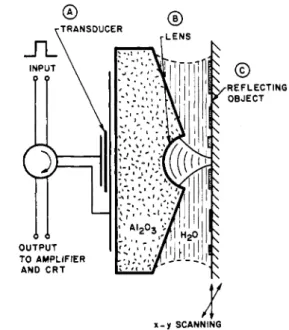
The acoustic components of the microscope are shown in Fig. 2 for the transmission mode. A photograph of the me- chanical components for

this

mode is presented in Fig. 3. The essential parts of the reflection mode microscope are shown in Fig. 4.

Referring to Fig. 2, we b.egin with the electrical input signal to the piezoelectric transducer. It is a sputtered film of zinc oxide sandwiched between the two films of gold. This transducer is extensively used in a variety of microwave acoustic devices [ 2 7 ] . It has proved to be efficient (50-percent conversion effective) and it operates at frequencies that exceed 10 GHz. In our instrument it generates a plane wave that travels through the sapphire crystal to the spherical lens. The ratio of

x

x - y SCANNING

FG. 4. Sketch of microscope components for reflection. the radius of the transducer to that of the lens as well as the transducer-lens spacing must be carefully adjusted. The lens is in the Fresnel zone of the radiating transducer and it is sur-

prisingly easy to pick a combination of dimensions that wlli result in nonuniform illuminations of the lens. At the lens surface the impedance ratio between sapphire and water is nearly 50 : 1 and t h i s must be overcome with a quarter-wave matching layer. Various combinations have been suggested- gold-quartz [281

,

glass [29]

,

Arsenic-Tri-Selenide 1171

-

and they all are effective. Carbon films with an acoustic imped- ance of 9 X lo6 kg/m2-s may be ideal for this purpose but they have not yet been used.

With the sapphire-water combination the beam converges to a focus with a focal length that is 15 percent greater than the radius of curvature. In the transmission mode (Fig. 2) the radiation passes through the object which is supported on a thin Mylar film and it is collected by an output-lens-transducer combination that is similar to the input. In this mode where we use continuous radiation it is possible to monitor either the change in amplitude or the change in phase of the signal as the object is scanned.

(4)

QUATE et al.: ACOUSTIC MICROSCOPY WITH MECHANICAL SCANNING 1095 r - - - -

-

1 I AI I I I I r MASTER CRYSTAL CLOCK I ! a95- 1.25 GHZ I S 8 H 4 BPF I , / I CRT DISPLAY

-

t

SCAN CONTROL - M x ) CRT DRIVE CIRCUITRY .-c

[

-

I

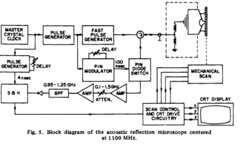
A

Fig. 5. Block diagram of the acoustic reflection microscope centered at 1100 MHz.

The object itself is mechanically translated through the beam waist by the loudspeaker shown in Fig. 3. This unit moves the object with simple harmonic motion along a straight line at a frequency of 60 Hz over a distance of 0.2 mm. A micrometer drive is used to lift the loudspeaker through this same distance in a time equal t o several seconds.

This slow scan speed (5-10 slframe) makes it necessary to store the image by some method before display. We use two methods: 1) a scan converter, and 2) direct writing on film.

In the reflection mode (Fig. 4) the radiation is pulsed so that the reflection from the object can be distinguished in time from spurious pulses that come from other reflecting points within the system. A block diagram of the reflection mode system is shown in Fig. 5. An avalanche transistor pulser excites the piezoelectric transducer through the circulator. The pulsewidth is selected such that the frequency content of the pulse covers the operating frequency range of the acoustic system.

As an example, a pulse of duration 500 ps can excite the acoustic system centered at 1100 MHz. The return pulse will then be an RF pulse centered at 1100 MHz and of a duration determined by the bandwidth of the acoustic transducer. After being amplified this pulse is detected and its amplitude is used to modulate the intensity (Z-axis) of a television monitor. The images are recorded by photographing the face of this monitor [ 301

.

In addition to a system with increased scan speed, other systems have been explored with features that complement and enhance those discussed here. Two are of primary interest. The nonlinear system where the output transducer is tuned to the second harmonic of the input; in this system the nonlinear properties of the object itself can be monitored [ 3 1

1.

In another system the

axis

of the output lens is moved from the colinear alignment as shown in Fig. 2 to

an

off-axis position

1321. It is then possible to detect the energy that is scattered through a wide angle by the object. It is analogous to dark field imaging in some ways since the output transducer does not detect the direct signal from the input when the object is absent.

Iv.

PROPERTIES OF ACOUS'ITC WAVES

It may, at first, seem U M ~ C ~ S S U Y t o write down the elemen-

tary equations for acoustic waves-no one would take the space t o write out the equations for electromagnetic waves-but we feel that it would be useful since acoustic wave properties do

FT2

~~

EPUlLlBRlUM P L A N E S

Fig. 6. Sketch of planes and then displacement from equilibrium as used in derivation of wave equation.

not have the familiar ring of dielectric constant or permeabil- ity. For that reason we will write out the differential equations. The wave equations that come from these are convenient for defining the terms that we deal with throughout the text.

Acoustic waves come in a variety of forms-shear, longitudinal, and surface-but in liquids the longitudinal wave represents the only mode of propagation. We

will,

therefore, limit the discussion to longitudinal, or compressional, waves where the direction of the particle motion coincides with the direction of propagation.

In the sketch of Fig. 6 we illustrate two parallel planes spaced by a distance Az. The medium is liquid with a density PO. The stress on plane 1

,

denoted by T I , and on plane 2 by T2, represents the force per unit of area on these planes. The differential pressure, or net force, on this thin slice is Tl - T2. The net force acting to compress the slice is (-aT/az)Az since T2 is given by T1

+

(aT/az)Az. Compressive force will be

taken as positive. The mass per unit area of this slice is p o A z . Newton's Force Law gives us the relation

- (aT/az)az = p 0 a z a u l a t or

aT/az = -poaulat. (4-1)

Here U is the velocity of the material in the slab. It is to be distinguished from the wave U, velocity which will appear later. If plane 1 is displaced from its equilibrium value by an amount

5

the material velocity U is equal t o

at/&.

If the dis-

placement from equilibrium of plane 1

,

51, is equal t o

5'

,

the displacement of plane 2, the slab is merely translated along the z-axis. But if & is less than

51

the slab is compressed by an

amount f 1

-

f z = - ( a s / a z ) A z . The strain S is equal to ( f l -

(5)

1096 PROCEEDINGS OF THE IEEE, VOL. 67, NO. 8 , AUGUST 1979

D E N S I T Y ( 0 / c m 3 )

Fig. 7. Chart of material parameters for acoustic waves. (Courtesy

OK

C. Eggleton.) and invert the order of differentiation, we find

We can invoke Hooke’s Law, T = cS, and write

a u l a z =

- -

1 aT/at. (4-2)

C

Here c is the elastic constant for the liquid.

The two equations (4-1) and (4-2) give us the wave equations. We assume lossless one-dimensional propagating waves in the form exp ( - j ( k z - a t ) ) and the equations take the form

k T = WPOU

k U = ( a / c ) T . (4-3)

We find the relation for k to be of the form

k = = f a / v s (4-4)

where

vs

=

a.

With the forward wave ( k = +a/vs) we have T = U =

Zo U and with the backward wave ( k = - a / v s ) we have T = Here Z o ( E 6 ) is the characteristic impedance of the acoustic wave. It is related to the wave velocity through the relation ZO = pov,. These three parameters are conveniently plotted in the form as given in Fig. 7. There we see that the wave velocity (m/s) and acoustic impedance (kg/m2-s) for different materials can vary by more than a factor of ten. This

- z o

u.

large variation underlines the crucial difference between acoustic imaging and optical imaging. The index of refraction, which determines both the wave velocity and wave impedance for optical waves, varies by less than a factor of two from material- to-material. It is for thisreason the biological material exhibits a small contrast for optical waves and a large contrast for acoustic waves.

The similarity of (4-1) and (4-2) with the one-dimensional form of electromagnetic waves means that we can take over those solutions directly. The power flow for acoustic waves is given by

(4-5) The reflectivity of a wave at an interface by two materials of impedance Zol and Zo2 is given by

Ref = z02

-

ZOl

z02 +ZOl

(4-6a) and the transmission (amplitude) through the interface is given by

Trans = 2ZOl

ZOl + z02

(4-6b) It also follows that the reflection at an interface can be reduced and the transmission improved with a matching layer one quarter wave in thickness with an impedance equal t o ( Z O I 2 0 2 ) ” ~ .

It thus forms an acoustic antireflection coating [ 291.

The attenuation of these waves is included by rewriting the propagation in the form exp (+j(kz - at)) exp (-

aZ)

where

(6)

QUATE et al.: ACOUSTIC MICROSCOPY WITH MECHANICAL SCANNING 1097

TABLE I

COMPARISON OF CALCULATED AND EXPERIMENTAL VALUE^ OF

ATTENUATION AT 1 GHz (FROM WAUK [34])

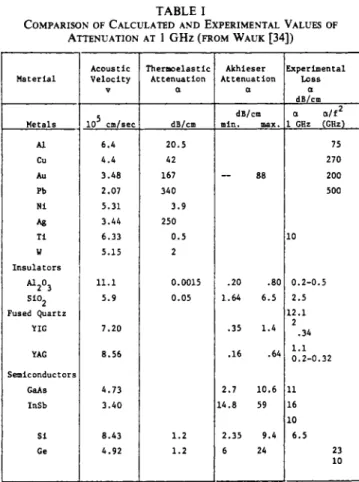
Material Hetals Al cu Au Pb Ni A8 Ti U Insulators A1203 sioz Fused Quartz Y IG YAG Semiconductors GaAS InSb si Ge Velocity Acoustic V 10’ cm/aec 6.4 4 . 4 3.48 2.07 5.31 3.44 6.33 5.15 11.1 5.9 7.20 8.56 4.73 3.40 8 . 4 3 4.92 rherwelastic Attenuation a dB/cm 20.5 42 167 340 3.9 250 0.5 2 0.0015 0.05 1.2 1.2 kt tenuation Akhieser a nin. max dBlcm I 88 .20 . 8 1.64 6.5 .35 1.4 .16 .6 2.7 10.6 4 . 8 59 2.35 9.4 6 24 3perimental Loss dB/cm 1 GHz (GHz) a elf2 Q 75 270 200 500 LO 0.2-0.5 2.5 12.1 2 .34 1.1 0.2-0.32 11 16 10 6.5 23 10

and dominant influence on acoustic imaging at microwave frequencies. Values for typical solids are shown in Table I.

In solids the attenuation is moderate and does not affect the microscope in an important way. But in liquids the attenuation is the factor that determines the ultimate resolution of the microscope. It is interesting, and somewhat ironic, to learn that this parameter-utterly different from the physical factors that limit the resolving power of an optical microscope- operates in such a way as to limit the resolving power of the acoustic instrument to a value near the optical limit.

In metals and certain other solids a major source of attenuation is due to thermoelastic heat flow [ 3 3 ] . A longitudinal wave has alternating regions of compression and rarefaction. Compression can produce an increase in temperatures and the flow of heat from this heated region to the cooler region at the rarefaction point represents a source of energy loss. The path length for heat flow of this sort decreases as the frequency increases. This produces a loss per cycle which increases directly as frequency, and hence the overall attenuation increases as the square of the frequency. The values of attenuation as

measured by Wauk 1341 for two important metals, Au and Ti, are given in Fig. 8.

In insulators an important source of attenuation has been worked out by Akhieser [351. It can be described in terms of viscous damping of the propagating sound waves due to the “phonon gas,” and the phonon-phonon collisions within this gas. Those materials included in Table I show the dramatic decrease from the values for metals. Semiconductors have attenuation coefficients which are intermediate between these values.

The theory that underlies the absorption in liquids is incom- plete and we must, therefore, lean heavily on the experimental data [ 3 6 ] . Liquids that appear suitable for the acoustic cell

1

LONGITUDINAL ATTENUATION IN TITANIUM 500 lo00 2000 FREOUENCY I M H z ) (a) 200

-

LONGITUDINAL ATTENUATION ROOM TEMPERATURE IN GOLD

-

90- z- 8 0 -

E

70-

2

6 0 - $ 50- a w I- SLOPE 1.97 40

t

3 0 1

I I , I l l 400 Mo 600 800 lo00 FREOUENCY ( M H z ) @) [ 341 1.

Fig. 8. Attenuation characteristics of (a) titanium and (b) gold (”auk

can be placed into three groups-1) water where a/fz is inde- pendent frequency (it also has a negative temperature coefficient), 2) liquids such as benzene and carbon disulphide which have a strong molecular absorption near 10’ Hz (and a positive- temperature coefficient), and 3) cryogenic liquids such as argon and helium.

The characteristics of water are shown

in

Fig. 9 where we see the reduced absorption with elevated temperature [28]. The

velocity does increase slightly with heating but it is not an important effect. The high attenuation at low temperatures is attributed to a component in the liquid with an ice-like open structure. It has been found that the absorption coefficient near room temperature can be reduced by as much as a factor of two with the addition of an electrolyte [ 371. It means that

saline solutions can be used in connection with biological systems.

In the second category we find liquids with a lower velocity than water but a low-frequency absorption that is enormous. This high value of attenuation comes from molecular vibration near 100 MHz. For selected liquids it can be described by a single relaxation time constant 7 or more conveniently by a critical frequency fc = 1361. The absorption is frequency dependent and takes on the following form

a / f 2

= B + ~ ( 1 +

(f/fCY).

In typical cases A is three orders of magnitude larger than B ,

(7)

1098 PROCEEDINGS OF THE IEEE, VOL. 61, NO. 0 , AUGUST 1919 1550

-

u

..

- ₁₅₀₀

₂

-

20 40 60 80 I00

Fig. 9. Acoustic wave properties of water as a function of temperature (Lemons [21]).

1250F

0 I 1 I

L

A

lo7 lo8 lo9 IOIO

(a) f , Hz f i ) f , Hz 6400

:::K!

1600 0

lo6 lo7 lo8 lo9 IOIO 10"

(c) f , Hz

Fig. 10. Absorption characteristics for liquid described with a single relaxation time (Fabelinskii [36]). (a) Methylene chloride. (b)

Benzene. (c) Carbon disulfide.

can neglect the A coefficient in the absorption. The experimental curves taken from the work of Fabelinskii (and repro- duced in Fig. 10) [ 36

I ,

are typical of liquids with a single relaxation frequency. The liquid carbon disulphide is interesting at high frequencies since the attenuation and the velocity are

both less than water. It is a classic example of high absorption arising from molecular vibrations. In this case it is a bending mode of the CS, molecule which peaks near 78 MHz [331. In Fig. 11 we show on an enlarged scale, the comparative absorp- tion of CS, near 3 GHz.

These curves are significant in our work for a most interesting reason. The high-frequency limit is not known for many liquids, and for those liquids where it has been measured, the accuracy is not high. The work in liquids for frequencies greater than 4 GHz has been carried out through Brillouin scattering of laser beams. With this technique liquids with

I I

I 2 3

ACOUSTIC FREOUENCY (GHrl

Fig. 11. Detail of absorption characteristic for carbon disulphide as compared to water (Attal [ 311).

low attenuation coefficients

(a/f2

<

5 X 1 0 - l ~ ) are difficult to measure since this corresponds to the limit imposed by the linewidth of the laser itself. If you were optimistic by nature (as we are!), this would suggest that more work needs to be done in this frequency range using the direct method of monitoring of absorption in a variable length acoustic cell.

At cryogenic temperatures liquids have both low attenuation and low velocity [ 21. Two hold promise-argon with a velocity of 0.86 X lo5 cm/s, and superfluid helium with a velocity of

0.24 X l o 5 cm/s. But we will not dwell on these possibilities since a discussion of operation at cryogenic temperatures is outside the scope of this review.

The examples included here offer some hope that a liquid might be found with a velocity near lo5 cm/s and a value of

a/f2

less than 5 X lo-' sz /cm. If a liquid with these properties could be found it would permit us to operate the microscope with a wavelength of 0.25 pm.

V.

CONVERGING

BEAMS A . Spatial Frequencies

In 1973, Cathey wrote 1391

The impression o f information onto an electromagnetic wave by modulating some parameter, such as amplitude, frequency, or phase, as a function of time is a familiar concept. Spatial infor- mation can also be impressed on the wave by amplitude, fre- quency, or phase modulation.

. . .

He goes on in Qlapter 5 to introduce the concept of spatial frequencies and he illustrates how these procedures can be used to deal with imaging problems. In earlier work, Goodman

[401 and O'Neill [411 made extensive use of the spatial frequency concept to analyze systems for imaging. A large part of

this later writing used the work of Ratcliffe [421 as a source. Ratcliffe's article is so clearly written and it sheds so much light on spatial frequency decomposition that it is s t i l l today well worth reading. Champeney [431 has discussed the comparative merits of the classical approach using diffraction inte- grals of this approach based on angular spectrum and spatial frequencies.

(8)

QUATE e t d.: ACOUSTIC MICROSCOPY WITH MECHANICAL SCANNING 1099

X

4

T R A N S M I T T I N G TRANSDUCER

Fig. 12. Sketch for a plane wave in x-z plane showing h, and h, as 0 , ky = 0, and k , = 2n/A, = kg cos x. Wave equatlon demands that components of LO. For this wave kg = 2n/ho, kx.= 2n/hx = ko cos

k i + k $ + k z = k g .

The sketch of Fig. 12 shows the appropriate geometry for a plane wave propagating as

exp (-jot

+

jko cos Ox + j k o cos xz) = exp ( - j u t

+

jk,x +jk,z) where

X.

is the freespace wavelength and 8,

x,

k,, and k, are defined in Fig. 12. We willhereafter suppress the exponential time factor and use the following notations:

u amplitude distribution of the actual function of both A spectrum of plane waves that are used to constitute the

x a n d y ;

spatial distribution u. It is a function of k, and k,.

These two are related via the Fourier transform and this will become clear as we proceed.

We first develop the relation between the spatial distribution and the angular spectrum for a system that is uniform in the y direction. We can, therefore, deal only with the x and z coordinates as indicated in Fig. 12. The amplitude of the plane wave components propagating at the angle 8 is denoted by A ( 8 ) d e , and the component directed along the z-axis is A ( @ sin 8 d e . These plane waves can be summed over 8 to form the spatial distribution of u ( x ) at z = 0

+n/2

U(X) = A ( 8 ) sin 8 exp (-jk,x) dB.

We note that k, will serve as well to denote this component

since k, = ko c o s 8. In this treatment where we deal with a single frequency ko is constant and we have therefore dk, = -sin 8 de ko. Equation (5-1) takes the form

I,,,

(5-1

1

u ( x ) =

--

rk0

A ( k , ) exp (-jk,x) dk,. ko - k ,

For k ,

>

ko the waves at z = 0 are evanescent and do not propagate. Nevertheless, they can be included without undue difficulty [441 and the limits can be extended to +m. After

suitable normalization, t h i s can be written as

u ( x )

=[I

A(k,) exp (-jk,x) dk,. (5-2) In this form we recognize that the spatial distribution at z = 0 is the Fourier transform of the angular spectrum distribution A(k,). 1t.follows directly from this that the angular spectrum'

SCANNED

OBJECT

Fig. 13. Sketch of imaging system showing the various planes beginning

with the input to plane 1 at the lens t o plane 3 at the focal point and frnally plane 6 at the output.

A ( k , ) is given by the inverse transform of u ( x ) . With a spatial distribution in both x and y , these results can be extended to give

+-

u(x,y)

=I--

A ( k , , k,) exp [ - j ( k , x

+

kyy) dkXdk,l (5-3)

and the inverse

1 +=

A ( k , , k,) = 7 u ( x , y ) exp [+j(k,x + kyy)l dx du.

(2n) -m

(5-4) In more compact notation, equation (5-3) becomes

U ( X , Y ) = F I A ( k x , k,)) (5-3a)

A@,, k,) = F - ' ( U ( x , Y ) )

.

(5-4a) and equation (5-4) becomes

The power of this analytical approach is evident when we consider the problem of determining the spatial distribution u l ( x , y ) across a plane 1 a distance z1 from the input plane. We know the distribution at the input plane to be u o ( x , y ) .

The appropriate geometry for our complete system is sketched in Fig. 13. With the decomposition into plane waves as treated in (5-3), we can easily see the change in each of the plane waves as they move from the input plane to plane 1. It is merely a phase shift given by

AI@,, k,) = A o ( ~ , , k,) exp [+jkzzll ( 5 - 5 )

where k, = (k;

-

k:

-

k;)'I2 as indicated in Fig. 12.

The most illustrative case and one that serves our purpose here is for a beam that is rather narrowly confined around the z-axis. In this case both k, and k, are small as compared to

ko and we have

The relation in ( 5 - 5 ) then becomes

(9)

1100 PROCEEDINGS OF THE IEEE, VOL. 67, NO. 8, AUGUST 1919 where Ao(kx, k,) is related to the spatial distribution at the

input plane by (5-4). The spatial distribution at the output plane is written with the aid of (5-6) in the form

X exp [-j(kxx

+

k,y)I dk, dk, (5-7)

or in compact notation we write

6 - 7 1

But we know from the theorems of Fourier transformation that

3

-l {ghl=

5-'

*

3-'

{ h ) (5-8) and

With these we can write in place of (5-7)

(5-1 0)

This permits us to move from the input plane to plane 1 just prior to the lens itself (see Fig. 13). In traversing the lens the angular spectrum is modified in phase according to the expression

exp[ 2 f

1

-iko(x2 + y 2 )

(5-1 I ) where f is the focal length of the lens (see Fig. 14). At the focal plane itself the distribution is u2 (x, y ) . It is equal to

Fourier transform of the spatial distribution at the lens input u l ( x , y ) as modified by the pupil function P(x1 ,y1). That is we can write

(5-1 2 )

where the transform is now limited by the pupil function to the region

In writing the pupil function in this way we have assumed that the diameter of the beam at the focal plane is much less than the radius of the lens R. In a generalized treatment the pupil function can include numerous interface factors such as the effect of a quarter-wave matching layer. From focal plane we

can with (5-1 0) determine the spatial distribution at a distance z from the focal plane. At that plane we encounter the object

a A A B / 9 / / / / - _I

Eg. 14. A lens acts to convert a spherical wavefront (A) into a plane wavefront (b). It must add a phase shift exp ( - j k o A ) where f'

+

? = ( f + A)' - f + 2Afor A = ?/2f= (x'

+

y')/2f.

which either described by a transparency t(x, y ) for the trans- mission mode or a reflectivity 9((x,y) for the transmission mode.

After traversing the object, or being reflected by the object, we can continue

this

process to again reach the focal plane, transform through the lens, and move from the lens to the transducer to obtain the distribution at plane 6 are denoted by us(x,y). This is the output, but it is not that parameter that we measure. Rather we measure the transducer voltage V .

This voltage is simply.the integral of the distribution u 6 ( x , r ) weighted by the response of the transducer itself at the point x and y , i.e., s(x, y ) :

V = ~ ~ u 6 ( x , y ) s ( x , Y ) d x d y . (5-1 3) It is easy to demonstrate that a unit voltage on the transducer will produce a wave distribution in the c r y s t a l , plane 0, that is just s(x, y ) . It has also been shown that the principal of reciprocity can be invoked to demonstrate this feature.

B. Beam Contours and Computed Images

The theory as outlined here can be used to calculate beam contours and spatial frequency content of the converging beam. With these we can compute the images that would be expected for idealized objects. The details of the calculations which do appear in the literature 1451 are not appropriate for this review and we

will,

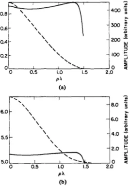
therefore, proceed directly to the results.

We specify a particular lens at a sapphire-water interface and a frequency of 1 GHz. The lens radius is 75 pm and the focal length is 83 pm. The radius of the transducer is 96 pm and it is spaced 2 mm from the lens. The sensitivity of the trans- ducer #(x, y ) is assumed to be uniform over the area of the transducer itself. The spatial frequency transfer function of the system produced by

this

combination is shown in Fig. 15. In Fig. 15(a) we plot amplitude (dotted) and phase (solid) as a function of the spatial frequencies for an ideal lens which neglects all factors such as absorption in the liquid, mode conversion at the lens surface, and a quarter-wave matching layer on this surface. When all of these factors are included the distributions change to that given in Fig. 15(b). The corresponding beam contours at the focal plane are shown

in Fig. 16. The expected resolving power for beam contoured

as in Fig. 16(b) is 0.7?10, i.e., the instrument is capable of resolving a periodic grating with a full period of 0 . 7 b which is 1 .O pm for the wavelength in water is 1.5 pm at 1 GHz.

(10)

QUATE et d.: ACOUSTIC MICROSCOPY WITH MECHANICAL SCANNING 1101 0.81 \ \ I \

\

.-

c e 0.41 \ \

'\

0.2

t

'\

6 0 I I

'\

I 0 0.5 I .o 1.5 2.0 l o

a

P i (a)

-

\ I I I

-

W

'

-

\ 6.0-

'

-

8.0

3

2.0

k

'.

-

%

\ \ E \ -6.0 .- \ \ 5.5

-

\ - 4.0 \ 3 0

.

_'.

_a 5.0 I I 0 0.5 1.0 1.5 2.0 P A @)

Fig, 15. The amplitude (dashed) and phase (solid) of the spatial fre-

quency transfer function in terms of the spatial frequency p and the wavelength A. Curve (a) is for an ideal system. Curve (b) is for a sys- tem with spherical aberration, mode conversion, and absorption in the liquid as described in the text.

p'

bL-J

2 1 01

L-J

1 2

( b r

Fig. 16. The amplitude distribution at the focal plane for the condi- tions specified in Fig. 1 5 .

The theory can also be used to calculate the expected re-

sponse of

an

edge and three different systems are compared in Fig. 17 [ 281. There we show a conventional incoherent and coherent optical system together with the coherent scanning system. We see that the confocal scanning system (Fig. 17(c)) compares with the incoherent conventional system. The ring- ing usually associated with coherent radiation (Fig. 17(a)) is missing. The characterizations as shown in Figs. 16 and 17 are often used but it is necessary to consider the image of

an

individual object with some care. For example, the circular sidelobes on the beam profie of Fig. 16 do not show up in the

-10 10-

c

Fig. 17. Calculated one-dimensional images of a step function object. (a) Conventional coherent image. (b) Conventional incoherent image. radiation (Lemons [ZS]).

(c) Image produced by a confocal scanning system using coherent

image of a straightedge as in Fig. 17. They could, however, distort the image of two scattering centers that were closely spaced when their scattering strengths were widely different.

A computed image of the red blood cell is shown in Fig. 18. The object is assumed to be lossless and it only acts to vary the phase of the transmitted beam as shown in Fig. 18(a). The transducer output is plotted in Fig. 18(b) for the phase of the signal and in Fig. 18(c) for the amplitude of the signal. The phase image Fig. 18(b) corresponds quite closely to the object itself. The amplitude image Fig. 18(c) exhibits high contrast even though the amplitude of the scanning beam was assumed to be uniform over the object. The amplitude image of phase objects of this kind does not necessarily conform to the structure of the object. This phenomenon is important for t h i s

type of imaging. It can be explained with the aid of the sketch in Fig. 19. We learn from that diagram that a change in object phase over the beam cross section will tilt the transmitted beam. After passing through the output lens the tilted beam will transform into a pseudo-plane propagating off the center of the crystal axis. It

will,

therefore, be normally incident on the transducer but the transducer response will be diminished

as a result of the tilting. The decrease in the magnitude of the output signal is proportional to the gradient of phase in the focal plane. The phase of the transmitted beam is unaffected

by

this

tilt. We do, therefore, expect the phase of the output

signal to reproduce the phase of the object with good fidelity.

(11)

1102 PROCEEDINGS O F THE IEEE, VOL. 67, NO. 8, AUGUST 1979

-T----l

Fig. 18. Ideal red blood cells. (a) Phase profde from Evans and Fung

[46] (hemoglobin absorption equal to water). (b) Phase response of transducer output. Grid lines are h/8 by All 6. (c) Amplitude response of transducer together with the derivative of the phase responses in (b). Grid lines are AI16 by h / 3 2 .

TRANSMITTER RECEIVER

I

4

SCANNED CBJECT

Fg. 19. Illustration of change in illumination of the lens when the beam encounters a transverse phase gradient in the focal plane. correspond to the phase gradients in the object plane. We see both of these features in Fig. 18(b) and (c).

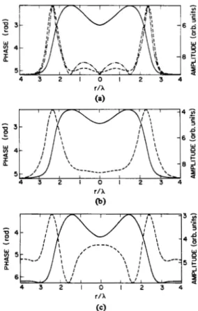
These ideal properties are changed if the focal conditions are not precise. Defocusing can be of two types-either a) the object is not placed at the focal plane, or b) the spacing between the lens in Fig. 13 does not equal to confocal conditions. These two defocusing conditions are illustrated as follows. In Fig. 20 we show the spatial frequency content of the beam for (a) the in-focus condition, (b) the object defocused from the focal plane by one wavelength, and (c) the lens sepa- ration is decreased from the confocal condition by one wavelength. There are changes in both the phase and amplitude of the spatial frequencies, and they alter the images as shown in Fig. 21. The translation of the object from the focal plane

I I v) - 8.0

.;i

6.0 - \ \ 0 2.

e

2 5.5

-

\ - 6 . 0 $ \

.-

\ w \ \ - 4.0

-

\ 3 W n \ \ \

-

2.0 t _d \ 5.0

-

I

,

- a

2

0 0.5 I .o 1.5 2.0 \ \

-

2.0 t _d \ 5.0

-

I

,

- a

2

0 0.5 I .o 1.5 2.0 I \ \ \ \ \ \ 2.0 -

-

1.0 k o '

P

'.

0. I 1

'.+

0 0.5 1.0 1.5 2.0 PA (c)

FII. 20. Spatial frequency transfer function amplitude (dashed line) and phase (solid line) for various cases. (a) Lenses are confocal and the object is at focus. (b) Lenses are confocal and the object is de- focused by one wavelength. (c) Transmitter-receiver lens spacing decreased by one wavelength.

makes a small difference in the contrast and broadens the image somewhat. But the more dramatic distinction comes from the images in Fig. 21(c), where the lens spacing is decreased by one wavelength. We see there in the amplitude image a contrast reversal which is different in character from the image. This type of reversal for focusing errors in optical systems has been discussed by Goodman [471.

Finally, in Fig. 22 we present the red blood cell images as they appear when the focusing errors of Fig. 21 are introduced. The most pronounced feature in this series is again the contrast reversal in the amplitude images when the lens spacing decreases (Fig. 22).

C. The

V(Z)

Curves

For the reflection instrument the output voltage as ex- pressed in (5-14) can be used in a unique way to measure some of the elastic properties of the reflecting surface. The

initial distribution at the transducer is ui(x, y ) , the distribution of the returning field is uO(x, y ) , and we have

In writing

this

form we are anticipating the fiial result wherein we monitor V as a function of the parameter 2 ; i.e., the dis-

(12)

QUATE et al.: ACOUSTIC MICROSCOPY WITH MECHANICAL SCANNING 1103

r/X

@)

r/X

( 4

Fig. 21. Computed amplitude (dashed line) and phase (solid line) images

of the ideal red blood cell with the conditions specified in Fig. 20. placement of the reflecting object from the focal plane. Equa- tion (5-14) can take on a more suitable form by using the transforms described previously. The details are published elsewhere [481. The final form for V ( 2 ) is as follows:

Since our problem exhibits circular symmetry about the z a x i s we can replace x' + y 2 by r2 and write [48]

(5-1 5)

An alternative form of this expression and its derivation may be found in the literature [491. This

V(Z)

expression has proved to be valuable as a method for studying surfaces. Some results for real cases will be given in a later section. Here we want to gain some understanding of what is to come by ana- lyzing a few simple reflectors.

One straightforward case is that of a lens with a uniform illumination, i.e., u1(r) = 1, and radius R , i.e., P ( r ) = circ ( r / R ) and a perfect reflector !TI(r/f) = 1. In this case (5-1 5) becomes

V ( 2 ) =

lR

r exp (-j r2) dr =

-

R 2 exp ( - j x ) sine x

2

(5-16)

PHASE AMPLITUDE

(c)

Fii. 22. Experimental imagea of red blood cells for the three conditions specified in Fig. 20. Note the r&rsal of contrast in amplitude for (c) the favorable comparison with the theory in

Fig.

2l(c).

-

MIRROR LENS DETECTOR

r R I A 8

=

f 2 / 2 z (From above,

r 2 + R ~( r + A ) ' = r 2 + 2 A r A = R~ / z r * ( R ' / f 2 1

z

(b)

Fig. 23. Sketch of rays for a displaced mirror. (a) Reflection from mirror displaced by z from the focal plane. (b) Phase variation across fransducer for a spherically diverging wave.

where

x E n ( R / f )2Z/xo and sinc x E sin x/x.

The result in (5-16) is easily understood. When Z is positive the wavefront that impinges on the transducer is spherical with a radius of curvature that depends on 2. As 2 is changed we experience an increasing number of cyclic variations of the field across the transducer which gives rise to the sinc curve.

It is instructive to use this concept and calculate the value of

2 for the f i i t null in the transducer output. The sketch in Fig. 23 is sufficient for this purpose. We can see from Fig.

(13)

1104

[FOCAL PLANE OF L E N S

PROCEEDINGS OF THE IEEE, VOL. 67, NO. 8, AUGUST 1979

R O + r y = ( R ~ + A ) ~ 2 R ~ + ~ A R ~ Z A = r: R0 = R~ r 2 / t 2

Fig. 24. Illustration of phase shifts associated with a spherical dome of radius R, centered on focal plane.

23(b) that the response of the transducer will be reduced to zero when the wave at the outer rim undergoes an additional phase shift of 27r as compared to the portion of the wave at the center of the transducer (A =

b).

We see from Fig. 23(a) that this occurs when the radius of curvature of the converging wave is adjusted to be R 2 / 2 b . From (b) we fiid that a displacement of the reflector from the focal plane by an amount Z wlliproduce a radius of curvature in the converging wave given by r = f 2/2Z. In turn

this

is equal t o R 2 / 2 b . Therefore, we have the expression Z = &(Rz/f 2, for the null condition

at the transducer. This agrees with (5-16) when we note that t h e ~ e c function has a null for x =

n

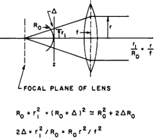
(and Z/)b = (R/f )2).

In the second example as illustrated in Fig. 24 the reflecting object is a dome with radius of R o and centered on the focal plane. We see from the sketch that oxf the plane spaced a distance Ro from the focal plane, the waves suffer an additional phase shift of ko(2A) where A is given by

The factor of 2A is entered since the wave going and returning traverses this distance twice. We are at liberty to represent

this dome by a surface with a reflectivity given by

91

= exp [-jko(F) 1.3

and in place of (5-16) we have

V(2) =

lR

r exp [-jko(F) r2] dr R 2 = - exp ( - j x 2 ) sinc x2 (5-17) 2 where x2 = n(R/fI2(Z +Ro)/)b.

This result is similar to (5-16) except that the reflector must be located at Z = -Ro to give the maximum output. This is intuitively correct since at that point the curvature of the dome equals the curvature of the wavefront.

For the third case we consider the special situation where the acoustic impedance of the liquid is equal to that of the solid. However, the velocity ratio is still small and the critical

Fig. 25. V(Z) curves of a uniformly illuminated lens for a perfect re- flector (solid line) and for a reflector matched to the liquid up t o a critical angle (dashed line).

angle for total internal reflection occurs within the conver- gence of our acoustic beam. (The interface between mercury and silicon approximates this condition.) The reflectance becomes

3={

0, r < R 1 1, R ~ < ~ < R '

For this case we can still use (5-17) except that the limits on the integration now extend from R 1 to R. The result is

V(2) =

-

R 2 - R : k o R 2 - R : sinc -

-.

(5-18) 2 2

f 2

It is similar to the f i i t case but the null now occurs at Z/x, = f2/(R2 - R:) which is larger than that of the perfect reflector.

A comparison of (5-18) with (5-16) is shown in F i g . 25 for the case where the area of transducer within R1 is equal to t h e a r e a b e t w e e n R 1 a t R , i . e . , R = f i R l .

For the fourth case we choose a reflector that more closely follows the characteristics of the actual liquid-solid interface encountered with real objects. The reflectivity for t h i s case

is of the form

With t h i s we can write

(5-19)

V(2) =

lR'

r exp [-j

(F)

1'3 dr

+

exp ( j # )

J"

exp

[

- j

(F)

1'1 dr.

R ,

This when evaluated reads

X exp (+j$) sinc - ko (R2 - R:)

2 f 2

(14)

QUATE et al.: ACOUSTIC MICROSCOPY WITH MECHANICAL SCANNING ₁₁₀₅

I

- 2

_I

_{I l i / I ?}

_ _

Fig. 26. V ( Z ) curve of a uniformly illuminated lens for a reflector with a unit amplitude reflectance function. Reflectance function phase is nonzero for angles exceeding a critical value. Different V ( Z ) curves are for various phase values.

The curves resulting from different values of $J are shown in

Fig. 26.

These simple cases tell us a great deal about the character we expect t o find in the measured V(2) curves. A reduction of the reflectivity for incident angles less than the critical angle will tend to broaden the curve and a phase shift for angles greater than the critical angle will tend t o displace the curves. There is one other important feature that comes forth- namely contrast reversal in the images as 2 is varied [ 151,

[50]. Assume that we have an image composed of two materials-one with the reflectivity as in the second case, and the other as in the perfect reflector. For 2 = 0 the perfect reflector would have the larger reflectivity and would appear brighter in the image (Fig. 25). For negative values of 2 we see that the contrast is reversed particularly at the null where the ideal reflector goes dark and the reflector with the matched liquid remains fairly bright.

The most important feature that has been left out of these examples is the nonuniform illumination of the lens. This can

arise from several factors: diffraction over the length of the crystal, a nonuniform response of the transducer over its cross section, the axis of the transducer displaced from the lens axis through misalignment in the initial fabrication, or the quarter- wave matching layer can exhibit inhomogeneities. For all of these reasons, and more, we find actual distributions t o differ from the ideal that has been postulated in the previous examples. The most pronounced effect in the V(2) curves is the disappearance of the nulls and their replacement with dips of varying degrees of depth.

D . Reflectance Functions

We now attend to the problem of calculating the reflectance of plane waves on a liquid-solid interface as a function of the angle of incidence. The problem is straightforward and it has been treated in the literature [ 51

I .

Our needs are somewhat peculiar in that we must cover the entire range of incident angles. The operating frequency is high enough to make the attenuation of the liquid important but for the most part we deal with a linear problem in classical wave theory. The prob- lem is sketched in Fig. 27. We express the reflected wave in terms of the incident wave by the reflection coefficient

3.

We require both the magnitude and the phase of %as the incident angle 0 (or more properly sin 0 ) is varied. In the solid we find that several modes can propagate which involve longitudi-

X I \ I I’

.

\ / I \ I , - 2 INCIDENT__.” \ \ \ \ \

Fig. 27. Acoustic plane wave scattering at a plane boundary between a liquid and an isotropic solid.

1 . 0 0

* I !

(b)

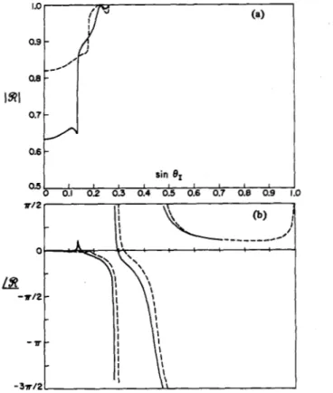
Fig. 28. Amplitude and phase of the reflectance function for H,O-YIG and H,O-YAG interfaces.

nal, shear, and Rayleigh waves along the interface. In layered media other modes representing energy propagating within the layer will enter.

For this review it is only required that we present the final form of the reflectance functions since it is this parameter that enters into the expression that we use t o calculate the

V(2) curves. A typical result is given in Fig. 28 for two differ- ent crystals (YAG and YIG) against water. The magnitude of

9

is rather uninteresting since the results would not be altered appreciably if we set % = 1 over the entire range. But the phase

9

is crucial. We see that the phase of the reflected wave under-

goes a large shift at the critical angle and approaches 2n for large angles. The range near the critical angle is important where the phase relation between the reflected wave and the incident wave undergoes a maximum of change. The boundary conditions that determine this condition require continu-