IET Radar, Sonar & Navigation
Research Article
Compressive sensing-based robust
off-the-grid stretch processing
ISSN 1751-8784 Received on 16th May 2017 Revised 4th August 2017 Accepted on 12th August 2017 E-First on 22nd September 2017 doi: 10.1049/iet-rsn.2017.0133 www.ietdl.org
Ihsan Ilhan
1, Ali Cafer Gurbuz
2, Orhan Arikan
31Department of Electrical and Electronics Engineering, TOBB University, Ankara, Turkey
2Department of Electrical and Computer Engineering, The University of Alabama, Tuscaloosa, AL, USA 3Department of Electrical and Electronics Engineering, Bilkent University, Ankara, Turkey
E-mail: [email protected]
Abstract: Classical stretch processing (SP) obtains high range resolution by compressing large bandwidth signals with narrowband receivers using lower rate analogue-to-digital converters. SP achieves the resolution of the large bandwidth signal by focusing into a limited range window, and by deramping in the analogue domain. SP offers moderate data rate for signal processing for high bandwidth waveforms. Furthermore, if the scene in the examined window is sparse, compressive sensing (CS)-based techniques have the potential to further decrease the required number of measurements. However, CS-based reconstructions are highly affected by model mismatches such as targets that are off-the-grid. This study proposes a sparsity-based iterative parameter perturbation technique for SP that is robust to targets off-the-grid in range or Doppler. The error between reconstructed and actual scenes is measured using Earth mover's distance metric. Performance analyses of the proposed technique are compared with classical CS and SP techniques in terms of data rate, resolution and signal-to-noise ratio. It is shown through simulations that the proposed technique offers robust and high-resolution reconstructions for the same data rate compared with both classical SP- and CS-based techniques.
1 Introduction
Obtaining higher resolution is important in many engineering applications such as remote sensing, medical and radar imaging. Radar systems are often operated with large bandwidths to provide high resolution. Classical matched filtering detects targets over the entire unambiguous range if Nyquist rate samples are acquired. This could require high data rates for large bandwidth waveforms. On the other hand, stretch processing (SP) [1–3] processes wide bandwidth signals with narrowband systems such as lower rate analogue-to-digital converters (ADCs) by constraining the observed range to a limited window and still obtains the high resolution of the wide bandwidth waveform. Therefore, SP is very well suited for target discrimination and classification [4], synthetic aperture radar (SAR) imaging [5] and tracking applications [6].
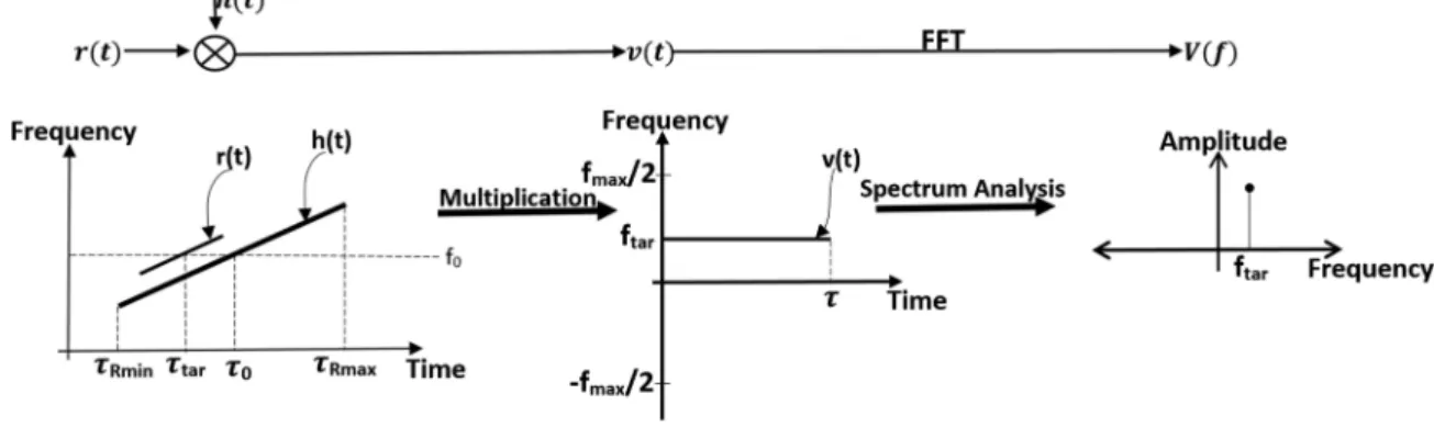
In general, linear frequency-modulated (LFM) waveforms are used in SP, and the received signal is stretched by mixing it with a local oscillator LFM signal that has the same sweep rate as the transmitted signal as illustrated in Fig. 1.
After the mixing operation, targets at different ranges appear at distinct frequencies. Classical SP determines these frequencies, and hence their corresponding ranges, by spectrum analysis techniques such as the discrete Fourier transform (DFT). The Doppler shift
due to moving targets causes frequency shifts which result in ambiguity in the observed ranges. SP using multiple pulses within a pulse–Doppler framework could estimate both range and velocities of moving targets by using two-dimensional (2D) spectral analysis [2, 7].
The range window observed by SP either has a small number of targets or a single target that has a small number of dominant reflecting points. In either case, the observed target scene can be sparsely modelled. Compressive sensing (CS) [8, 9] provides further reduction in the number of measurements for reconstruction of sparse signals under a known basis. Owing to the appealing properties of CS and its important advantages for radar, CS has received considerable attention in the radar research community. In [10], the possibility of sub-Nyquist sampling and elimination of match filtering has been discussed. CS has been shown great interest in many high-resolution radar imaging applications such as SAR imaging [11, 12], inverse SAR imaging [13], ground penetrating radar [14] and through-the-wall imaging [15].
The CS framework is also studied with SP in [16]. In this application of CS to SP the continuous frequency space is discretised into a frequency grid and the DFT basis is used only to reconstruct the discrete frequency/range vectors. If the scatterers are exactly on the ranges that correspond to the grid frequencies of
the CS dictionary, then the observed scene is sparse and CS reconstruction of the scene will be successful. However, no matter how fine the grid is, the targets are typically located in off-grid positions. It has been discussed in the literature that the off-grid targets create an important degradation in CS reconstruction performance [17–23] since the sparsity assumption on the defined grids is no longer valid. In [16], performance degradation for off-grid targets is discussed for CS and SP but a solution is not provided.
This paper proposes to use a parameter-perturbed orthogonal matching pursuit (PPOMP) technique [24] within the SP framework for robust and joint estimation of range and Doppler parameters of the targets for sparse reconstruction under the general off-grid case following an initial work in [25]. The proposed technique is analysed in terms of data rate, resolution and reconstruction performance for varying levels of noise and it is compared with classical SP- and CS-based approaches. It is shown that the proposed robust CS-based technique for SP provides better performing results in all compared metrics.
This paper is organised as follows: Section 2 describes the signal model, as well as classical SP- and CS-based SP frameworks. The proposed parameter perturbation technique and its application to SP are detailed in Section 3. Simulation results on a variety of examples with performance comparisons are given in Section 4 and Section 5 covers conclusions.
2 Signal model for SP
Assume that the radar transmits an LFM waveform as
s(t) = ejπαt2
rect tτT (1)
where B is the bandwidth, τT is the pulse width, α = B/τT is the sweep rate and rect(x) = 1, | x| ≤ 0.5 and 0 elsewhere. If there are
K scatterers at ranges Rk, k = 1, 2, …, K within the range interval [Rmin, Rmax] around centre range R0, the received signal r(t) from all reflectors will be modelled as
r(t) =
∑
k = 1 K
Akej2π fct−τRkejπα t−τRk2 (2) where fc is the carrier frequency, c is the propagation speed, Ak is the complex reflectivity and τRk= 2Rk/c is the time delay of the kth scatterer. This time delay can also be written with respect to the time delay τ0 for the centre range as
τRk= τ0+ ΔτRk. (3)
In SP, a heterodyne LFM signal h(t) with the same sweep rate as s(t) is formed
h(t) = ej2π fc(t−τ0)ejπα(t−τ0)2 (4) and is mixed with the received signal r(t) as illustrated in Fig. 1. The mixed output can be written as
v(t) = r(t)h∗(t) =
∑
k = 1 K A^ ke−j2παΔτRkt+ n(t) (5) where n(t) is the additive white Gaussian noise. The term A^k includes all complex constant terms for the scatterer. The mixer output is a sum of complex exponentials as observed from (5) and the frequency of the kth term that corresponds to a relative time delay ΔτRk is fRk= αΔτRk. The output of the mixer is sampled witha lower rate ADC where the sampling frequency is determined by the bandwidth in the mixed signal. Since the mixed signal is a sum of complex exponentials, its bandwidth is related to the maximum
and minimum possible frequencies which are determined by the range window extent. If the time delay interval for the examined range window is ΔτRint= τRmax− τRmin where τRmax and τRmin correspond to maximum and minimum time delay values for the corresponding maximum and minimum ranges in the range window; then a minimum ADC rate Fs= ΔτRintα is required in SP which is less than the pulse bandwidth B. Uniformly sampling the mixed output with Fs over a time interval of
τRmin−
τT
2 ≤ t ≤ τRmax+
τT
2 will generate at least
Ns≥ FsτT+ ΔτRint number of samples for SP. Target frequencies
fRk and their corresponding ranges are estimated with any spectrum
estimation technique such as DFT.
If targets are moving, frequency shifts occur due to Doppler, creating ambiguity in range estimation for a single pulse. To solve for both range and velocity pulse–Doppler processing is used with SP. In pulse–Doppler, a coherent train of Np pulses is transmitted. So, the data model in (5) can be rewritten as
v(t) =
∑
n = 0 Np− 1∑
k = 1 K A^ke−j2π fRktfej2π fDkts+ n(t) (6) where fDk is the Doppler frequency of individual scatterers within− PRF2 , PRF2 interval, tf is the fast time defined within
t0−τ2 ≤ t ≤ th 0+τ2h, ts= nTPRI, n = 0, 1, …, Np− 1 is the slow
time where TPRI and PRF = 1/TPRI are the uniform pulse repetition
interval (PRI) and pulse repetition frequency, respectively. Classical SP applies a 2D DFT to find both range and Doppler frequency parameters of individual scatterers.
The examined range window is generally populated with a small number of scatterers, hence application of CS-based techniques allow further decrease in data acquisition rates. Classical application of CS to SP requires discretisation of continuous frequency space where target range and velocity parameters live. Hence, a sparsifying basis is created where each column corresponds to the data model that is expected to be acquired for a target having on grid parameters. Under Nyquist rate sampling this is 2D DFT basis. However, for the sparsity assumption to hold, this model inherently assumes that the DFT grid points θj= fRj, fDj, and discrete target frequencies exactly
coincide.
Assuming the on grid model, the measurements v can be written as
v= Ψx + n (7)
where x is the discrete range–Doppler space and Ψ is the sparsity basis with columns being a(θk) = e−j2π fRtfej2π fDts. The size of Ψ will be NtNp× NRND where Nt is number of time samples, Np is
number of pulses and NR and ND are the number of frequency grid
points of range and Doppler, respectively.
If there are K scatterers that are exactly on grid, then x is a K-sparse vector. However, target range and velocity values may be anything from the continuous parameter space and v cannot be represented as K-sparse in Ψ which diminishes the benefits of CS.
In formulation of CS, lower rate linear measurements of the form are acquired
v= ΦΨx + n = Ax + n (8)
where Φ is a measurement matrix of size M × LtNp. Depending on
the implementation of the linear measurement setup, the Φ matrix can be populated with random Gaussian or Bernoulli entries or it can be random M rows of LtNp× LtNp identity matrix
corresponding to sampling at random times. In all cases the combined matrix A= ΦΨ should satisfy the restricted isometry property [26] for reconstruction of x from measurement v. The
sparse scene x can be obtained by solving an optimisation problem as
min
x ∥ x ∥1 s . t . ∥ v − Ax ∥2 ≤ ϵ . (9)
The problem in (9) can be efficiently solved with linear programming. Also many greedy sparse reconstruction techniques have been developed [27–30] for lower computational complexity.
3 Parameter perturbation for reconstruction
The model in (8) and the classical CS reconstruction in (9) assume on grid target parameters. However, the targets may have any range or Doppler parameter value and hence are essentially always off-the-grid. This off-grid problem invalidates the sparsity assumption with the previously used basis and hence degrades the reconstruction performance of CS solvers. Here, parameter-perturbed OMP (PPOMP) technique proposed in [24] is adapted and applied for robust reconstruction of sparse scenes in SP. The proposed algorithm is a greedy technique where at each iteration it starts with a selected set of on grid dictionary vectors that can be obtained via one of any known sparse reconstruction techniques such as OMP [27]. Therefore, at the kth iteration the measuredsignal can be represented as v= v⊥+
∑
i = 1 k
αia(θi), (10)
where v⊥ is the orthogonal residual of v to the span of k chosen
support vectors a (θi). The idea is to perturb the parameters θi in (10) such that the norm of the orthogonal residual is to be minimised; hence, the goal is to solve the following minimisation problem: arg min αk, δ fRk, δ fDk∥ v −i = 1
∑
k αia( fRi+ δ fRi, fDi+ δ fDi) ∥ s . t . |δ fRi| < ΔfR/2, |δ fDi| < ΔfD/2 (11)where δ fRi and δ fDi are the perturbation of range and Doppler of
the ith scatterer from the corresponding grid point, respectively.
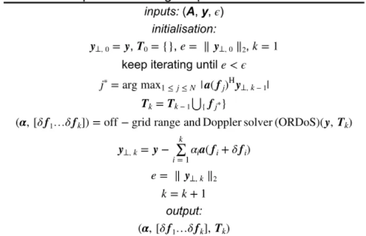
The proposed OMP-based iterative algorithm with the additional step of parameter perturbation giving a sub-optimal solution to (11) is summarised in Table 1.
For the solution of the non-convex optimisation problem defined in (11), an iterative optimisation of the cost function is proposed where selected dictionary parameters are iteratively
updated toward directions that decrease the residual norm while keeping them within their grids. To do so estimation of target reflectivities α and the parameter perturbations are iteratively performed. Starting from grid centres of corresponding k targets θi, 1= fRi, fDi, i = 1, 2, …, k, target reflectivity vector αℓ is
obtained for the given target parameters θi,ℓ as
αℓ= arg min
α ∥ v −i = 1
∑
kαi,la(θi,l) ∥2 (12) where ℓ is the perturbation index and i represents the target index. Starting from the k target grid parameters, at each perturbation step, parameters of all k targets are updated as
θi,ℓ+ 1= θi,ℓ+ δθi,ℓ, i = 1, …, k (13)
The parameter updates δθi,ℓ at the perturbation index ℓ can be
found by solving (see (14)) The target reflectivities in (12) are solved for using a standard least-square formulation. However, the problem defined in (14) is a constrained non-linear optimisation problem. For solving (14), a fRi, l+ δ fRi, fDi, l+ δ fDi is linearised
at the current parameter point as
a fRi, l+ δ fRi, fDi, l+ δ fDi ≃ a fRi, l, fDi, l
+ ∂a∂ f
Ri, lδ fRi+ ∂a∂ fDi, lδ fDi.
(15)
Hence using (15) in (14) results
[δθ1,ℓ…δθk,ℓ] = arg minu ∥ rℓ− Bℓu∥2 (16) where rℓ is the orthogonal residual defined as
rℓ= b −
∑
i = 1 k
αi,ℓa θi,ℓ
and Bℓ∈ CM× 2k is the matrix holding the weighted partial
derivatives at the linearisation point and is defined as Bℓ= ΔRα1,ℓ∂ f∂aR 1, l, …, ΔRαk,ℓ ∂a ∂ fRk, l, ΔDα1,ℓ∂ f∂aD 1, l, …, ΔDαk,ℓ ∂a ∂ fDk, l . (17)
Note that Bℓ is different at each perturbation iteration ℓ since the
linearisation points θi,ℓ are updated and a new linearisation is made
at each updated parameter point as stated in (15). Since directly using the solution from (16) could result in errors in parameter updates due to a first-order linear approximation, instead a gradient descent update that reduces the norm in (16) is adapted. The negative gradient direction that reduces the norm at u = 0 will be Re{2BlHrl} and the proposed parameter update is
αℓ= [a(θ1,ℓ)a(θ2,ℓ)…a(θk,ℓ)]†b (18a)
θi,ℓ+ 1= θi,ℓ+ μi,ℓRe{BℓHrℓ} (18b)
where μi,ℓ is the gradient descent step size. The proposed off-grid
parameter solver procedure is summarised in Table 2. Table 1 Proposed off-the-grid sparse solver
inputs: (A, y, ϵ) initialisation:
y⊥, 0= y, T0= {}, e = ∥ y⊥, 0∥2, k = 1
keep iterating until e < ϵ
j∗= arg max
1 ≤ j ≤ N|a( fj)Hy⊥,k− 1|
Tk= Tk− 1⋃{fj∗}
(α, [δ f1…δ fk]) = off − grid range and Doppler solver (ORDoS)(y, Tk)
y⊥,k= y − ∑ i = 1 k αia( fi+ δ fi) e = ∥ y⊥,k∥2 k = k + 1 output: (α, [δ f1…δ fk], Tk) [δθ1,l…δθk,l] = arg min δ fRi: |δ fRi| ≤ ΔfR/2 δ fDi: |δ fDi| ≤ ΔfD/2 ∥ v −
∑
i = 1 k αi,la fRi, l+ δ fRi, fDi, l+ δ fDi ∥ 2 . (14)4 Simulation results
In this section, performance of the proposed technique is analysed for SP in the case of targets that have arbitrary range or Doppler parameters. In the comparisons, an SP framework is developed. A linear chirp waveform with bandwidth of B = 20 MHz and pulse width τT= 100 μs is used. Hence sweep rate is α = 0.2 MHz/μs. The range window centre is taken to be 1.5 km, with an extent of 1.5 km around the centre. The range resolution will be ΔR = 7.5 m corresponding Δ fR= 50 kHz and range window is discretised to
range grids with ΔR.
In addition, Np= 16 pulses are used with PRI of 1 ms, hence
PRF is 1 kHz. Doppler space is uniformly discretised to ND= 32
Doppler grid points within −PRF/2, PRF/2 . If classical SP is used, a sampling frequency of Fs= ΔτRintα = 2 MHz would be required to reconstruct the observed limited range window instead of sampling at the waveform bandwidth of B = 20 MHz. Further
reduction in number of samples with CS is tested where CS uses only a random subset of these measurements in the simulations.
First, a sparse scene with K = 6 scatterers is simulated using the
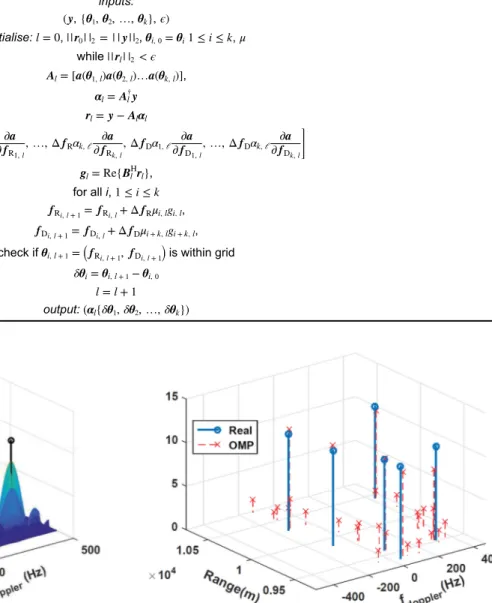
defined parameters. Additive white Gaussian noise is added with a signal-to-noise ratio (SNR) of 20 dB. A surface clutter model defined as in [7] is also generated and added to the measurements with an signal-to-clutter ratio (SCR) of 15 dB. Classical SP obtains the result in Fig. 2. It can be seen that a non-sparse scene is generated with SP. In this case, SP uses DFT which is a matched filtering operation resulting in sinc shape sidelobes. In addition,
performing DFT degrades considerably if random subsamples are observed instead of full Nyquist samples. For classical CS and the proposed PPOMP techniques, only 10% of the time samples are used. Both techniques use the same measurements and have the same stopping criteria. The obtained reconstruction results for CS and PPOMP are shown in Figs. 3 and 4, respectively. Correct target parameters are also plotted in these figures as circles for better comparison. It can be seen that while PPOMP generates a correct sparse scene, classical CS generates a non-sparse scene due to the off-grid nature of the targets. In addition, CS only returns the grid centres as parameter estimate values, while PPOMP could provide off-grid target parameter estimates.
Next for quantitative analysis, the proposed PPOMP technique is compared with standard SP, OMP and ℓ1-based reconstruction techniques for varying sparsity, SNR and measurement rate levels. In each test, 50 independent trials are performed and target parameters are selected randomly. Sparsity-based techniques are terminated if the energy of residual signal is under a given threshold. To measure the off-grid parameter estimation performance of compared techniques Earth mover's distance (EMD) [31] metric is used. EMD is a measure of minimum mass flow between two compared scenes and it is more appropriate compared with a mean squared error (MSE) since our goal is to capture the off-grid parameter estimation performance.
First, effect of scene sparsity level is analysed. All techniques are simulated using 20% of the entire set of measurements at an SNR of 20 dB and SCR of 15 dB for varying sparsity levels from Table 2 Off-grid RDoS
inputs:
(y, {θ1, θ2, …, θk}, ϵ)
initialise: l = 0, ||r0| |2= | | y||2, θi, 0= θi1 ≤ i ≤ k, μ while ||rl| |2< ϵ
Al= [a(θ1,l)a(θ2,l)…a(θk,l)],
αl= Al†y rl= y − Alαl Bl= Δ fRα1,l∂ f∂a R1, l, …, Δ fRαk,ℓ ∂a ∂ fRk, l, Δ fDα1,ℓ ∂a ∂ fD1, l, …, Δ fDαk,ℓ ∂a ∂ fDk, l gl= Re{BlHrl}, for all i, 1 ≤ i ≤ k fRi, l + 1= fRi, l+ Δ fRμi,lgi,l, fDi, l + 1= fDi, l+ Δ fDμi+k,lgi+k,l, check if θi,l+ 1= fRi, l + 1, fDi, l + 1 is within grid
δθi= θi,l+ 1− θi, 0
l = l + 1 output: αl{δθ1, δθ2, …, δθk}
Fig. 2 Classical SP result applying 2D DFT using all measurements.
Obtained EMD is 13 dB Fig. 3 OMP result using only 10% of all measurements. Obtained EMD is−6 dB
10 to 100 point reflectors. The average EMD is shown in Fig. 5 for each technique. It can be observed that the proposed technique achieves lower EMD values for all sparsity levels compared with tested techniques. EMD for SP is much higher compared with all sparsity-based techniques since it generates a non-sparse scene and its EMD value is affected the least from changing sparsity level of the scene. While EMD increases for sparsity-based techniques as the sparsity of the scene increases, PPOMP still achieves lower values compared with classical OMP or ℓ1-based reconstruction techniques.
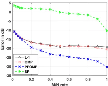
Second, measurement rates, M/N, is varied between 0.01 and 1
for a fixed setting of K = 30 targets with an SNR of 20 dB and SCR of 15 dB. Obtained average EMD values are presented in Fig. 6. It is seen that for measurement rates higher than 0.1 the proposed technique provides lower EMD values than compared techniques. Increasing the number of measurements lowers EMD for the proposed method while OMP and ℓ1 techniques level off since they only provide on grid solutions. While increasing M/N
ratio decreases EMD for SP, still it is much higher compared with sparsity-based techniques.
Next, all techniques are compared for varying SNR levels of −10to 30 dB at a fixed setting of K = 40 and M/N = 0.2 for sparsity-based techniques. All measurements are used in classical SP. Average EMD results for compared techniques are given in Fig. 7. It can be observed that while SP uses all measurements it provides higher EMD values compared with all sparsity-based techniques since it does not provide sparse results. PPOMP provides lower EMD for SNRs higher than 0 dB. While increasing SNR helps to lower average EMD for PPOMP, EMD does not get smaller for other techniques. This shows that off-grid estimation performance gets better with increasing SNR with the proposed
technique while classical sparsity-based techniques only provide on grid results hence EMD stays similar after some SNR level.
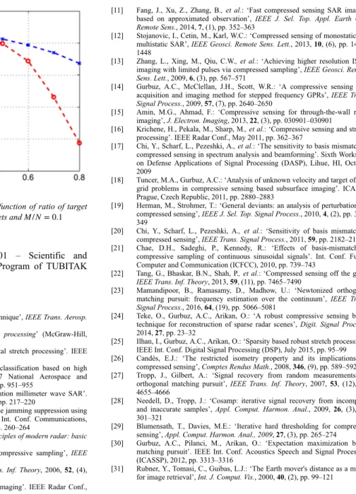
For resolution analysis of compared techniques, a two-target scenario with same Doppler but varying ranges is performed. Two targets are randomly located at different ranges with a distance of
R1, 2 which is less than a resolution level of ΔR. Classical OMP and PPOMP techniques are compared using a finer grid size. The average MSE in the target parameter estimates as a function of ratio of target distance R1, 2 to range resolution level ΔR is shown in Fig. 8. It can be seen that when targets are separated more than half of the grid size, parameter estimation error for the proposed technique is much smaller compared with OMP result. This shows that the proposed technique provides better separation of targets when the target separation is lower than the classical match filter resolution limit.
5 Conclusion
It is shown that the moderate data rate offered by classical SP for high bandwidth waveforms can be further reduced by the CS-based techniques. Although classical CS techniques provide advantages over SP, it has off-the-grid target problems which reduce its performance. The proposed sparsity-based PPOMP technique is robust to targets off-the-grid in range or Doppler and successfully recovers the sparse scenes. It is shown through simulations that the proposed technique offers robust and high-resolution reconstructions for the same data rate compared with classical SP-and CS-based techniques.
Fig. 4 PPOMP result using only 10% of all measurements. Obtained EMD
is −21 dB
Fig. 5 Average EMD for tested techniques for different sparsity levels
Fig. 6 Average EMD for tested techniques for different measurement rates
6 Acknowledgment
This work was supported by the 1001 – Scientific and Technological Research Projects Funding Program of TUBITAK with grant no. 113E515.
7 References
[1] Caputi, W.J.: ‘Stretch: a time-transformation technique’, IEEE Trans. Aerosp. Electron. Syst., 1971, AES-7, (2), pp. 269–278
[2] Richards, M.: ‘Fundamentals of radar signal processing’ (McGraw-Hill, 2005)
[3] Schikorr, M.: ‘High range resolution with digital stretch processing’. IEEE Radar Conf., May 2008, pp. 1–6
[4] Hu, R., Zhu, Z.: ‘Researches on radar target classification based on high resolution range profiles’. Proc. IEEE 1997 National Aerospace and Electronics Conf. NAECON, July 1997, vol. 2, pp. 951–955
[5] Brehm, T., Wahlen, A., Essen, H.: ‘High resolution millimeter wave SAR’. European Radar Conf. EURAD., October 2004, pp. 217–220
[6] Ying, X., Xiukai, Y., Yongqiang, Z., et al.: ‘Noise jamming suppression using stretch processing and BEMD filtering’. 2013 Int. Conf. Communications, Circuits and Systems, November 2013, vol. 2, pp. 260–264
[7] Richards, M.A., Scheer, J.A., Holm, W.A.: ‘Principles of modern radar: basic principles’ (SciTech Publishing, 2010)
[8] Candes, E., Wakin, M.: ‘An introduction to compressive sampling’, IEEE Signal Process. Mag., 2008, 25, (2), pp. 21–30
[9] Donoho, D.: ‘Compressed sensing’, IEEE Trans. Inf. Theory, 2006, 52, (4), pp. 1289–1306
[10] Baraniuk, R., Steeghs, P.: ‘Compressive radar imaging’. IEEE Radar Conf., April 2007, pp. 128–133
[11] Fang, J., Xu, Z., Zhang, B., et al.: ‘Fast compressed sensing SAR imaging based on approximated observation’, IEEE J. Sel. Top. Appl. Earth Obs. Remote Sens., 2014, 7, (1), pp. 352–363
[12] Stojanovic, I., Cetin, M., Karl, W.C.: ‘Compressed sensing of monostatic and multistatic SAR’, IEEE Geosci. Remote Sens. Lett., 2013, 10, (6), pp. 1444– 1448
[13] Zhang, L., Xing, M., Qiu, C.W., et al.: ‘Achieving higher resolution ISAR imaging with limited pulses via compressed sampling’, IEEE Geosci. Remote Sens. Lett., 2009, 6, (3), pp. 567–571
[14] Gurbuz, A.C., McClellan, J.H., Scott, W.R.: ‘A compressive sensing data acquisition and imaging method for stepped frequency GPRs’, IEEE Trans. Signal Process., 2009, 57, (7), pp. 2640–2650
[15] Amin, M.G., Ahmad, F.: ‘Compressive sensing for through-the-wall radar imaging’, J. Electron. Imaging, 2013, 22, (3), pp. 030901–030901
[16] Krichene, H., Pekala, M., Sharp, M., et al.: ‘Compressive sensing and stretch processing’. IEEE Radar Conf., May 2011, pp. 362–367
[17] Chi, Y., Scharf, L., Pezeshki, A., et al.: ‘The sensitivity to basis mismatch of compressed sensing in spectrum analysis and beamforming’. Sixth Workshop on Defense Applications of Signal Processing (DASP), Lihue, HI, October 2009
[18] Tuncer, M.A., Gurbuz, A.C.: ‘Analysis of unknown velocity and target off the grid problems in compressive sensing based subsurface imaging’. ICASSP, Prague, Czech Republic, 2011, pp. 2880–2883
[19] Herman, M., Strohmer, T.: ‘General deviants: an analysis of perturbations in compressed sensing’, IEEE J. Sel. Top. Signal Process., 2010, 4, (2), pp. 342– 349
[20] Chi, Y., Scharf, L., Pezeshki, A., et al.: ‘Sensitivity of basis mismatch to compressed sensing’, IEEE Trans. Signal Process., 2011, 59, pp. 2182–2195 [21] Chae, D.H., Sadeghi, P., Kennedy, R.: ‘Effects of basis-mismatch in
compressive sampling of continuous sinusoidal signals’. Int. Conf. Future Computer and Communication (ICFCC), 2010, pp. 739–743
[22] Tang, G., Bhaskar, B.N., Shah, P., et al.: ‘Compressed sensing off the grid’, IEEE Trans. Inf. Theory, 2013, 59, (11), pp. 7465–7490
[23] Mamandipoor, B., Ramasamy, D., Madhow, U.: ‘Newtonized orthogonal matching pursuit: frequency estimation over the continuum’, IEEE Trans. Signal Process., 2016, 64, (19), pp. 5066–5081
[24] Teke, O., Gurbuz, A.C., Arikan, O.: ‘A robust compressive sensing based technique for reconstruction of sparse radar scenes’, Digit. Signal Process., 2014, 27, pp. 23–32
[25] Ilhan, I., Gurbuz, A.C., Arikan, O.: ‘Sparsity based robust stretch processing’. IEEE Int. Conf. Digital Signal Processing (DSP), July 2015, pp. 95–99 [26] Candès, E.J.: ‘The restricted isometry property and its implications for
compressed sensing’, Comptes Rendus Math., 2008, 346, (9), pp. 589–592 [27] Tropp, J., Gilbert, A.: ‘Signal recovery from random measurements via
orthogonal matching pursuit’, IEEE Trans. Inf. Theory, 2007, 53, (12), pp. 4655–4666
[28] Needell, D., Tropp, J.: ‘Cosamp: iterative signal recovery from incomplete and inaccurate samples’, Appl. Comput. Harmon. Anal., 2009, 26, (3), pp. 301–321
[29] Blumensath, T., Davies, M.E.: ‘Iterative hard thresholding for compressed sensing’, Appl. Comput. Harmon. Anal., 2009, 27, (3), pp. 265–274 [30] Gurbuz, A.C., Pilanci, M., Arikan, O.: ‘Expectation maximization based
matching pursuit’. IEEE Int. Conf. Acoustics Speech and Signal Processing (ICASSP), 2012, pp. 3313–3316
[31] Rubner, Y., Tomasi, C., Guibas, L.J.: ‘The Earth mover's distance as a metric for image retrieval’, Int. J. Comput. Vis., 2000, 40, (2), pp. 99–121
Fig. 8 MSE of range parameter estimates as a function of ratio of target distance to range resolution level with K = 2 targets and M/N = 0.1