Feedforward controller synthesis for uncertain time delay systems via dynamic iqcs

(1)

T.C.

YILDIZ TECHNICAL UNIVERSITY

GRADUATE SCHOOL OF NATURAL & APPLIED SCIENCES

FEEDFORWARD CONTROLLER SYNTHESIS

FOR UNCERTAIN TIME DELAY SYSTEMS VIA DYNAMIC IQCs

LEVENT UCUN

DANIŞMANNURTEN BAYRAK

PHD THESIS

DEPARTMENT OF ELECTRICAL ENGINEERING

CONTROL AND AUTOMATION PROGRAM

YÜKSEK LİSANS TEZİ

ELEKTRONİK VE HABERLEŞME MÜHENDİSLİĞİ ANABİLİM DALI

HABERLEŞME PROGRAMI

ADVISOR

ASSOC. PROF. İBRAHİM BEKLAN KÜÇÜKDEMİRAL

İSTANBUL, 2011DANIŞMAN

DOÇ. DR. SALİM YÜCE

İSTANBUL, 2012

(2)

T.C.

YILDIZ TECHNICAL UNIVERSITY

GRADUATE SCHOOL OF NATURAL & APPLIED SCIENCES

FEEDFORWARD CONTROLLER SYNTHESIS

FOR UNCERTAIN TIME DELAY SYSTEMS VIA DYNAMIC IQCs

The Ph.D. study prepared by Levent UCUN has been approved by the jury given below as Ph.D. THESIS in Yıldız Technical University Graduate School of Natural and Applied Sciences Electrical Engineering Department on 10/01/2012.

Thesis Advisor

Assoc. Prof. İbrahim Beklan KÜÇÜKDEMİRAL Yıldız Technical University

Jury Members

Prof. Leyla Gören SÜMER

Istanbul Technical University _____________________

Prof. Galip CANSEVER

Yıldız Technical University _____________________

Assoc. Prof. Mehmet Nur Alpaslan PARLAKÇI

İstanbul Bilgi University _____________________

Assoc. Prof. Haluk GÖRGÜN

Yıldız Technical University _____________________

Assoc. Prof. İbrahim Beklan KÜÇÜKDEMİRAL

(3)

This PhD Thesis was partially supported by The Scientific and Technological Research Council of Turkey (TUBITAK) under Grant 108E089.

(4)

PREFACE

I would like to appreciate Assoc. Prof. İbrahim Beklan KÜÇÜKDEMİRAL who encourages and supports me during my Ph.D. study. I am also grateful to Prof. İbrahim Emre KÖSE for his valuable contribution to the thesis.

I also appreciate TÜBİTAK for the financial support that they have given during our research project.

Moreover, I am so thankful to my family who have been always understanding and supportive to me during my entire education period including my Ph.D. study.

Finally, I feel so lucky and happy that my dear wife Rabia UCUN has been always by my side whenever I need her support. I am so grateful to her for everything she has done for me.

January, 2012 Levent Ucun

(5)

v

LIST OF SYMBOLS

Suspension damping ratio daug Diagonal augmentation diag Diagonal

G Nominal system Hilbert Space Inertia of

Spring constant of the active suspension system Wheel spring constant

Sprung mass Unsprung mass

Order of the multiplier

Number of positive eigenvalues Number of negative eigenvalues Set of real numbers

sat Saturation function sup Supremum

x State vector y Measured output

Exogenous controlled output Constant time delay

Upper bound of time delay gain

Bounded and causal operator Multiplier

Initial condition Vector 2-norm

Off-diagonal block completion of a symmetric matrix

Spaces of vector-valued square integrable functions defined on Inner product

Extended imaginary axis Kronecker product

(8)

viii

LIST OF ABBREVIATIONS

BRL Bounded Real Lemma FB Feedback Controller FF Feedforward Controller FWM Free Weighting Matrix

IQC Integral Quadratic Constraints KYP Kalman Yakubovich Popov LMI Linear Matrix Inequalities

NFDE Neutral Functional Differential Equation RFDE Retarded Functional Differential Equation L-K Lyapunov-Krasovskii

(9)

ix

LIST OF FIGURES

Page

Figure 3. 1 Basic Feedback Configuration. ... 19

Figure 3. 2 Robust analysis problem. ... 24

Figure 4. 3 Robust feedforward problem ... 33

Figure 5. 4 Combined feedback and feedforward control scheme. ... 39

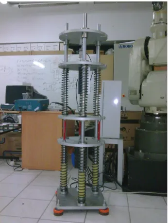
Figure 5. 5 Active suspension system experimental model. ... 42

Figure 5. 6 Random road profile. ... 44

Figure 5. 7 Bode magnitude plots of uncontrolled, only FB controlled and FF+FB controlled systems. ... 44

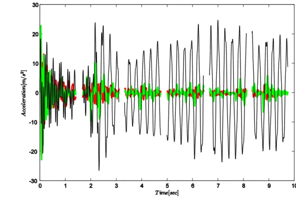
Figure 5. 8 Acceleration of the main body. ... 45

Figure 5. 9 Time-domain response. ... 48

Figure 5. 10 Comparison of FF+FB and only FB in terms of variation of z2(t). ... 50

Figure 7. 11 Simulink .mdl file for state and control delay example. ... 68

Figure 7. 12 Simulink .mdl file for neutral system example... 76

(10)

x

LIST OF TABLES

Page

Table 5. 1 Minimum allowable values for FB+FF and only FB in Example 1. ... 41

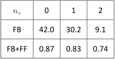
Table 5. 2 The obtained values of with respect to . ... 41

Table 5. 4 The obtained values of for ship steering problem without time-delay. .. 46

Table 5. 5 The obtained values of for ship steering problem with time-delay. ... 46

Table 5. 7 The obtained values of with respect to ... 48

Table 5. 9 The obtained values of with respect to . ... 50

(11)

xi

ÖZET

BELİRSİZLİK İÇEREN ZAMAN GECİKMELİ SİSTEMLER İÇİN DİNAMİK

ENTEGRAL KARESEL KISITLAR KULLANILARAK İLERİ-BESLEMELİ

DENETLEYİCİ TASARIMI

Levent UCUN

Elektrik Mühendisliği Anabilim Dalı Doktora Tezi

Tez Danışmanı: Doç. Dr. İbrahim Beklan KÜÇÜKDEMİRAL

Bu doktora tezi çalışmasında durumlarında ve kontrol sinyalinde zaman gecikmesi bulunan ve durumların türevlerinin (dinamiklerinin) zaman gecikmesi tarafından etkilendiği, literatürde "nötral" sistemler olarak da ele alınan sistemler için zaman gecikmesine bağlı gürbüz en iyi ileri-beslemeli ve geri-beslemeli denetleyici tasarımı üzerine çalışılmıştır. Ele alınan sistem aynı zamanda bozucular tarafından etkilenmektedir. Amaçlanan denetleyici tasarımı, durum geri beslemeli denetleyici ve dinamik ileri-beslemeli denetleyici olmak üzere iki temel kontrol döngüsü içermektedir. Geri beslemeli denetleyici ele alınan nominal sistemi kararlı kılma problemi için bir çözüm oluştururken ileri-beslemeli denetleyici bozucunun sistem çıkışına olan etkilerini minimize etmektedir. Frekansa bağlı çarpanlar (multiplier) içeren dinamik entegral karesel kısıtlar (EKK) sistemde bulunan zaman gecikmelerini ve sisteme etki eden parametrik belirsizlikleri ifade etmek için kullanılmışlardır. Kullanılan IQC'lerde bulunan çarpanların dereceleri elde edilen sonuçlardaki tutuculuğu azaltmak üzere mümkün olduğu mertebede yükseltilmişlerdir. Belirsiz zaman gecikmeli sistemin en küçük bozucu bastırma seviyesi ile evrensel ve asimtotik kararlı olmasını sağlayan gecikmeye bağlı yeter koşul, doğrusal matris eşitsizlikleri cinsinden verilmiştir. Doktora tezinin son bölümlerinde önerilen tasarımın başarımını göstermek için pek çok sayısal örnek verilmiştir.

(12)

xii

Anahtar Kelimeler: Zaman Gecikmeli Sistemler, İleri-beslemeli Denetleyici, Integral

Karesel Kısıtlar, Dayanıklı Kontrol, Optimal Kontrol

(13)

xiii

ABSTRACT

FEEDFORWARD CONTROLLER SYNTHESIS

FOR UNCERTAIN TIME DELAY SYSTEMS VIA DYNAMIC IQCs

Levent UCUN

Department of Electrical Engineering PhD. Thesis

Advisor: Assoc. Prof. Dr. İbrahim Beklan KÜÇÜKDEMİRAL

The thesis studies the design problem of a delay-dependent robust optimal feedforward plus feedback controller for systems having state and control delays and neutral systems with delays affecting the derivative of states. The controlled system having parametric uncertainties is subject to disturbances. The proposed controller involves two main control loops which are state-feedback and dynamic feedforward controller. The state feedback controller is used as a stabilizing controller whereas the feedforward controller performs the minimization of disturbance effects. Dynamic Integral Quadratic Constraints (IQCs) which consist of frequency dependent multipliers, have been introduced to represent the delays and parametric uncertainties in the system. The degree of the multipliers used in IQCs is increased in order to decrease the conservatism in the obtained results. Sufficient delay dependent criterion in terms of Linear Matrix Inequalities (LMIs) such that uncertain time-delay system is guaranteed to be globally, asymptotically stable with a minimum disturbance attenuation level, is presented in this study. Many numerical examples provided at the end, illustrating the usefulness of the proposed design.

(14)

xiv

Key words: Time-Delay Systems, Feedforward Controller, Integral Quadratic

Constraints, Robust Control, Optimal Control

YILDIZ TECHNICAL UNIVERSITY GRADUATE SCHOOL OF NATURAL AND APPLIED SCIENCES

(15)

1

SECTION 1 INTRODUCTION

1.1 Literature Review

Many physical systems such as chemical engineering processes, electrical networks and systems with long transmission lines involve time-delay naturally. This fact is one of the main reasons for instability and poor control performance.

There are many studies in the literature which survey the work on time-delay systems such as [1], [2], [3] and [4]. For example, after presenting some motivations for the study of time-delay system, [2] recalls modifications (models, stability, structure) arising from the presence of the delay phenomenon. A brief overview of some control approaches is provided, together with control methods of time-delay systems. Lastly, some open problems such as the constructive use of the delayed inputs, the digital implementation of distributed delays, the control via the delay, and the handling of information related to the delay value are discussed.

Moreover, [4] considers methods such as the time-domain control of delayed systems and the robust filtering including Robust Kalman filtering and robust filtering. The book begins with an introduction to time-delay systems and continues with the robust control of time-delay systems which involves robust stability, guaranteed cost control, passivity analysis and synthesis.

In the last decade, there has been a considerable amount of research effort in the literature for the analysis and design of robust controllers both for continuous and

(16)

2

discrete time-delay systems. These research activities can be classified basically into two main groups such as delay-dependent and delay-independent controller synthesis. Since it is a fact that delay-independent results tend to be more conservative, the researchers dealing with time-delay systems mostly deal with delay-dependent methods. In these studies, the delay systems are generally treated in time-domain by the use of different choice of Lyapunov-Krasovskii functionals [5], [6], [7], [8].

For example, [5] considers the problem of delay-dependent robust control for uncertain systems with time-varying delays. An improved delay-dependent bounded real lemma (BRL) for time-delay systems is established in terms of a linear matrix inequality. Based on the obtained BRL, a delay-dependent condition for the existence of a state feedback controller, which ensures asymptotic stability and a prescribed performance level of the closed-loop system for all admissible uncertainties, is proposed in terms of a matrix inequality.

Similarly, [6] discusses the problem of delay-dependent robust control for uncertain singular systems with time-delay. Firstly, based on Jensen inequality formula and Lyapunov stability theory, the sufficient condition is established for a delay-dependent singular system with time-delay, which guaranteed the nominal system to be regular, impulse free and stable. Secondly, based on the sufficient condition, the design method of robust state feedback controller is given for delay-dependent uncertain singular systems with time-delay, which guarantees that, for all admissible uncertainties, the resultant closed-loop system is regular, impulse free, and stable. [7] studies the design problem of a robust delay-dependent controller for a class of time-delay control systems with time-varying state and input delays, which are assumed to be noncoincident. Based on the selection of an augmented form of Lyapunov–Krasovskii (L-K) functional, first a Bounded Real Lemma (BRL) is obtained in terms of linear matrix inequalities (LMIs) such that the nominal, unforced time-delay system is guaranteed to be globally asymptotically stable with minimum allowable disturbance attenuation level. Extending BRL, sufficient delay-dependent criteria are developed for a stabilizing controller synthesis involving a matrix inequality for

(17)

3

which a nonlinear optimization algorithm with LMIs is proposed to get feasible solution to the problem. Moreover, for the case of existence of norm-bounded uncertainties, both the BRL and stabilization criteria are easily extended by employing a well-known bounding technique.

An alternative delay-dependent controller design is proposed for linear, continuous, time-invariant systems with unknown state delay in [8]. The resulting delay-dependent control criterion is obtained in terms of Park's inequality for bounding cross term. controller determined by a convex optimization algorithm with linear matrix inequality (LMI) constraints, guarantees the asymptotic stability of the closed-loop systems and reduces the effect of the disturbance input on the controlled output to within a prescribed level.

The common and main purpose of these studies is to design a control scheme that provides minimum gain and maximum allowable delay bound together with the minimum conservativeness.

Rather than using Lyapunov-Krasovskii functional approach, in the thesis, time-delay phenomenon is treated by means of IQCs. It is well-known that IQCs have played an efficient role especially in analysis of uncertain linear systems since the mid of 1990s. Survey paper [9] is a well-known reference for the use of IQCs and their applications. The paper introduces a unified approach to robustness analysis with respect to nonlinearities, time variations, and uncertain parameters. It is also shown how a complex system can be described, using IQCs for its elementary components. A stability theorem for systems described by IQCs is presented that covers classical passivity/dissipativity arguments but simplifies the use of multipliers and the treatment of causality. The paper contains a summarizing list of IQCs for important types of system components.

Although IQCs have been widely used especially in the stability analysis of dynamical systems, the use of IQCs in the synthesis of robust controllers is still a challenging and mostly an open problem. To the best of authors knowledge, there are only a few results on this subject in the literature. Among these few studies, one can list the following results such as [10], [11] and [12].

(18)

4

Particularly, [10] deals with the design problem of controllers for linear systems having actuator saturation nonlinearity. They establish IQC-based conditions under which an ellipsoid is contractively invariant for a single input linear system under a saturated linear feedback law. While the advantages of the proposed IQC approach remain to be explored, it is shown in the paper that the largest contractively invariant ellipsoid determined by this approach is the same as the one determined by the existing approach based on expressing the saturated linear feedback as a linear differential inclusion (LDI), which is known to lead to less conservative result in determining the largest contractively invariant ellipsoid for single input systems. However, their method is based on the use of static IQCs rather than dynamic ones which mostly leads to conservative results.

Different from [10], there is a couple of studies in the literature dealing with time-delay systems via dynamic IQCs such as [11] and [12]. These papers describe a set of delay-dependent IQC’s for time-delay uncertainty. The set is linearly parameterized in terms of the frequency-response of a complex valued multiplier. Using LMI optimization techniques, one may compute optimal multipliers and thereby obtain less conservative IQC stability robustness bounds for systems with uncertain time-delays. However, these researches focus on analysis rather than synthesis.

There are also some very few studies in the literature which deal with controller synthesis via dynamic IQCs. For instance, [13] studies robustness analysis with integral quadratic constraints, where they formulate a new positivity condition on the solution of the corresponding LMI which is necessary and sufficient for nominal stability of the underlying system. The application of the technical result is illustrated by a complete solution of the -gain and robust -estimator design problems if the uncertainties are characterized by dynamic integral quadratic constraints.

[14] and [15] deal with the feedforward dynamic controller synthesis for uncertain linear time invariant systems by the means of dynamic IQCs. They use IQCs for describing the uncertainty blocks in the system. A convex solution to the problem is obtained by using a state-space characterization of nominal stability that have been developed recently. Specifically, the solution consists of LMI conditions for the

(19)

5

existence of a feedforward controller that guarantees a given gain for the closed-loop system.

1.2 Purpose of Thesis

Inspired by the work in the literature, in this thesis, a robust feedforward controller design problem for uncertain time-delay systems via dynamic IQCs is considered. Many different types of time-delay systems such as state-delay systems, control-delay systems and neutral systems have been analyzed and used in this study. The control scheme proposed in the thesis can be configured for many different types of time-delay systems mentioned above. Hence, even if there are some differences in the time-delay systems that the proposed controller is applied, the controller can be configured easily to accomodate for a different type of time-delay systems. Another important point that we consider in this thesis is the parametric uncertainty that affects the system. By utilization of dynamic IQCs, we can configure a dynamic feedforward controller that deals with both time-delay and parametric uncertainty. Also, another important fact is that, the proposed controller scheme can be easily adjusted to be used for a reference tracking problem althouh it is mainly aimed to deal with the disturbance attenuation problem. Hence, the controller construction proposed in the thesis, can be employed for both reference tracking and disturbance attenuation problems.

One of the main advantages to use dynamic IQCs for feedforward controller design is that different types of time-delay systems, nonlinearities and uncertainties can be handled by a single dynamic IQC. In order to perform this technique, we use combination properties of dynamic IQCs which will be explained in due course.

On the other hand, one of the most important problems that we should deal with, is the reduction of conservatism in design. As it is mentioned in the literature, the IQCs are very elegant mathematical tools which are used to describe uncertainties and nonlinearities in the system, in a way which is suitable to be used with the theory of linear system. Hence, in order to obtain better controllers, we should avoid unnecessary conservatism as much as possible while using the IQCs. For this purpose, during the design of the feedforward controller, we use dynamic multipliers instead of

(20)

6

static ones. Another important point that might reduce conservatism is the selection of feedback controller in the system. Although the only assumption regarding the feedback controller is to make the closed-loop system stable, one might choose or design a high performance dynamic(static) feedback controller to reduce the conservatism. At this point, one can use less conservative feedback controllers such as suboptimal controllers which have been designed by using recent L-K functionals from literature.

1.3 Hypothesis

The proposed control scheme is based on several ideas: First, the proposed controller is in the form of two degree of freedom control configuration which consists of feedback and feedforward loops. Feedback controller deals with the stabilization of the nominal system and feedforward controller which is supposed to be a robust optimal disturbance attenuator, is used to improve the disturbance attenuation performance of the system. Second, the parametric uncertainty and time delay affecting states and control signal are described as dynamic IQCs in the controller synthesis. Finally, a convex optimization method is presented which accommodates the advantage of adjusting the degree of dynamic multipliers to reduce the conservatism as much as possible.

Hence, we are able to prove that we construct a feedforward controller that guarantees the uncertain time-delay system to be globally, asymptotically stable with a minimum disturbance attenuation level.

The contribution of the thesis to the control theory literature is the new general design method of a feedforward plus feedback controller loop for different kinds of uncertain time-delay systems by use of dynamic IQCs. Another important contribution of the thesis is the implementation and use of the combination of two or more dynamic multipliers for a controller design which is actually one more step forward than the usage of a couple of multipliers for stability analysis in the literature.

(21)

7

SECTION 2 TIME-DELAY SYSTEMS

One of the main reasons of instability and poor performance in many physical and dynamical systems, is the time-delay phenomenon concerning feedback control systems. Time-delay operator affecting the systems can be divided into two groups. Basically, the first group consists of the delays affecting system states and control signal applied to the system. The second group involves neutral systems which means that the delay operator is effective on state derivatives in the state dynamics.

In many physical and biological phenomena, the rate of variation in the system state depends on the past states. This characteristic is called a delay or a time delay, and a system with a time delay is called a time-delay system. Time-delay phenomena was first discovered in biological systems and was later found in many engineering systems, such as mechanical transmissions, fluid transmissions, metallurgical processes, and networked control systems. It is often a source of instability and poor control performance. Time-delay systems have attracted the attention of many researchers because of their importance and widespread occurrence. Basic theories describing such systems were established in the 1950s and 1960s. They covered topics such as the existence and uniqueness of solutions to dynamic equations, stability theory for trivial solutions. That work laid the foundation for the later analysis and design of time-delay systems.

Robust control of time-delay systems has been a very active field for the last 20 years and has spawned many branches, for example, stability analysis, stabilization design, control, passive and dissipative control, reliable control, guaranteed-cost control,

(22)

8

filtering, Kalman filtering and stochastic control. Regardless of the branch, stability remains the most significant objective. From this point of view, important developments in the field of time-delay systems that explore new directions have generally been launched from a consideration of stability as the starting point. This section of the thesis reviews methods of studying the stability of time-delay systems.

2.1 Brief History of Time-Delay Systems

Stability is a very basic issue in control theory and has been extensively discussed in many monographs [16], [17], [18]. Research on the stability of time-delay systems began in the 1950s, first by using frequency-domain methods and followed later also by using time-domain methods. Frequency-domain methods determine the stability of a system from the distribution of the roots of its characteristic equation or from the solutions of a complex Lyapunov matrix function equation [19]. This technique is mostly suitable for systems with constant delays. The main time-domain methods are generally based on Lyapunov-Krasovskii functional and Razumikhin function methods [20]. They are the most common approaches to the stability analysis of time-delay systems. Since it was very difficult to construct Lyapunov-Krasovskii functionals and Lyapunov functions until the 1990s, the stability criteria obtained were generally in the form of existence conditions; and it was impossible to derive a general solution. Then, Riccati equations, linear matrix inequalities (LMIs) [21] and Matlab toolboxes came into use; and the solutions they provided were used to construct Lyapunov-Krasovskii functionals and Lyapunov functions. These time-domain methods are now very important in the stability analysis of linear systems. This part reviews methods of examining stability and their limitations.

Consider the following linear system with a delay

(2.1) where is the state vector; is a delay in the state of the system, that is, it is a discrete delay; is the initial condition; and and are the system matrices. The future evolution of this system depends not only on its present

(23)

9

state, but also on its history. The main methods of examining its stability can be classified into two types; frequency-domain and time-domain.

2.1.1 Frequency Domain Methods

Frequency-domain methods provide the most sophisticated approach to analyzing the stability of a system with no delay . The necessary and sufficient condition for the stability of such a system is . When , frequency-domain methods yield the result that system (2.1) is stable if and only if all the roots of its characteristic function,

(2.2) have negative real parts. However, this equation is transcendental, which makes it difficult to solve. Moreover, if the system has uncertainties and a time-varying delay, the solution is even more complicated. Thus, the use of a frequency-domain method to study time-delay systems has serious limitations.

2.1.2 Time Domain Methods

Time-domain methods are based primarily on two famous theorems, the Lyapunov-Krasovskii (L-K) stability theorem and the Razumikhin theorem. They were established in the 1950s by the Russian mathematicians Krasovskii and Razumikhin, respectively. The main idea is to obtain a sufficient condition for the stability of system (2.1) by constructing an appropriate L-K functional or an appropriate Lyapunov function. This idea is theoretically very important; but until the 1990s, there was no good way to implement it. Then the Matlab toolboxes emerged and made it easy to construct Lyapunov-Krasovskii functionals and Lyapunov functions, thus greatly promoting the development and application of these methods. Since then, significant results have continued to appear one after another [22]. Among them, two classes of sufficient conditions have received a great deal of attention. One class is independent of the length of the delay and its members are called delay-independent conditions. The other class makes use of information on the length of the delay, and its members are called delay-dependent conditions.

(24)

10

The Lyapunov-Krasovskii functional candidate is generally chosen to be

(2.3) where and are to be determined and are called Lyapunov matrices and denotes the translation operator acting on the trajectory, for some (non-zero) interval . Calculating the derivative of along the solutions of system (2.1) and restricting it to less than zero yield the delay-independent stability condition of the system.

Since

(2.4) is linear with respect to the matrix variables and , it is called an LMI. If the LMI toolbox of Matlab yields solutions to (2.4) for these variables, then according to the Lyapunov-Krasovskii stability theorem, system (2.1) is asymptotically stable for all

and furthermore, an appropriate Lyapunov-Krasovskii functional is obtained. Since delay-independent conditions contain no information on delay, they are overly conservative, especially when the delay is very small. This consideration has given rise to another important class of stability conditions, namely, delay-dependent conditions, which do contain information on the length of a delay. First of all, they assume that system (2.1) is stable when . Since the solutions of the system are continuous functions of , there must exist an upper bound, , on the delay such that system (2.1) is stable for all . Thus, the maximum allowable upper bound on the delay is the main criterion for judging the conservativeness of a delay-dependent condition. The hot topics in control theory are delay-dependent problems in stability analysis, robust control, control, reliable control, guaranteed-cost control, saturation input control, and chaotic-system control.

Since the 1990s, the main approach to the study of delay-dependent stability has involved the addition of a quadratic double-integral term to the Lyapunov-Krasovskii functional (2.2)

(25)

11 where

(2.6) where derivative of is

(2.7) Delay-dependent conditions can be obtained from the Lyapunov-Krasovskii stability theorem. However, how to deal with the integral term on the right side of (2.7) is a problem. So far, three methods of studying delay-dependent problems have been developed, the discretized Lyapunov-Krasovskii functional method, fixed model transformations and parameterized model transformations.

The main use of the discretized Lyapunov-Krasovskii functional method is to study the stability of linear systems and neutral systems with a constant delay. It discretizes the Lyapunov-Krasovskii functional and the results can be written in the form of LMIs [23], [24] and [25]. The advantage of doing this is that the estimate of the maximum allowable delay that guarantees the stability of the system is very close to the actual delay bound. The drawbacks are that it is computationally expensive and that it cannot easily handle systems with a time-varying delay. Consequently, this method has not been widely studied or used since it was first proposed by Gu in 1997 [23].

2.2 Models of Time-Delay Systems

This section presents some basic definitions and theoretical results in the theory of time-delay systems.

In science and engineering, differential equations are often used as mathematical models of systems. A fundamental assumption about a system that is modeled in this way is that its future evolution depends solely on the current values of the state variables and is independent of their history. For example, consider the following first-order differential equation

(26)

12

The future evolution of the state variable at time depends only on and , and does not depend on the values of before time .

If the future evolution of the state of a dynamic system depends not only on current values, but also on past ones, then the system is called a time delay system. Actual systems of this type cannot be satisfactorily modeled by an ordinary differential equation; that is, a differential equation is only an approximate model. One way to describe such systems precisely is to use functional differential equations.

In many systems, there may be a maximum delay, . In this case, we are often interested in the set of continuous functions that map to , which we denote simply by . For any , any continuous function of time

and , let be the segment of given

by . The general form of a retarded functional

differential equation (RFDE) (or functional differential equation of retarded type) is (2.9) where and . This equation indicates that the derivative of the state variable at time depends on and for . Thus, to determine the future evolution of the state, it is necessary to specify the initial value of the state variable, , in a time interval of length , say, from to ; that is,

(2.10)

where is given. In other words, .

It is important to note that, in an RFDE, the derivative of the state contains no term with a delay. If such a term does appear, then we have a functional differential equation of neutral type. For example,

(2.11) is a neutral functional differential equation (NFDE). For an , a function is said to be a solution of RFDE (2.9) in the interval if is continuous and satisfies that RFDE in that interval. Here, the time derivative should be interpreted as a one-sided derivative in the forward direction. Of course, a solution also implies that is within the domain of the definition of . If the solution also satisfies the initial

(27)

13

condition (2.10), we say that it is a solution of the equation with the initial condition (2.10), or simply a solution through . We write it as when it is important to specify the particular RFDE and the given initial condition. The value of

at is denoted by . We omit and write or when is clear from the context.

A fundamental issue in the study of both ordinary differential equations and functional differential equations is the existence and uniqueness of a solution. We state the following theorem without proof.

Theorem 2.1 (Uniqueness) [26] Suppose that is an open set, function is continuous, and is Lipschitzian in in each compact set in . That is, for a given compact set, , there exists a constant such that

(2.12)

for any and . If , then there exists a unique solution

of RFDE (2.9) through .

2.2.1 Concept of Stability

Let be a solution of RFDE (2.9). The stability of the solution depends on the behavior of the system when the system trajectory, , deviates from . Without loss of generality, we assume that RFDE (2.9) admits the solution , which will be referred to as the trivial solution. If the stability of a nontrivial solution, , needs to be studied, then we can use the variable transformation to produce the new system

(2.13) which has the trivial solution .

For the function , define the continuous norm to be

(2.14) In this definition, the vector norm represents the 2-norm .

We now define various types of stability for the trivial solution of time-delay system (2.9).

(28)

14

Definition 2.1 [27]

 If, for any and , there exists a such that implies for , then the trivial solution of (2.9) is stable.

 If the trivial solution of (2.9) is stable, and if, for any and any , there

exists a such that implies , then the

trivial solution of (2.9) is asymptotically stable.

 If the trivial solution of (2.9) is stable and if can be chosen independently of , then the trivial solution of (2.9) is uniformly stable.

 If the trivial solution of (2.9) is uniformly stable and if there exists a such that, for any , there exists a such that implies for , and , then the trivial solution of (2.9) is uniformly asymptotically stable.

 If the trivial solution of (2.9) is (uniformly) asymptotically stable and if can be an arbitrarily large, finite number, then the trivial solution of (2.9) is globally (uniformly) asymptotically stable.

 If there exist constants and such that

(2.15) Then the trivial solution of (2.9) is globally exponentially stable; and is called the exponential convergence rate.

2.2.2 Lyapunov-Krasovskii Stability Theorem

Just as for a system without a delay, the Lyapunov method is an effective way of determining the stability of a system with a delay. When there is no delay, this determination requires the construction of a Lyapunov function, , which can be viewed as a measure of how much the state, , deviates from the trivial solution. Now, in a delay-free system, we need to specify the future evolution of the system beyond . In a time-delay system, we need the “state” at time for that purpose; it

(29)

15

is the value of in the interval . So, it is natural to expect that, for a time-delay system, the Lyapunov function is a functional, , that depends on and indicates how much deviates from the trivial solution. This type of functional is called a Lyapunov-Krasovskii functional. More specifically, let be differentiable; and let be the solution of RFDE (2.9) at time for the initial condition . Calculating the time derivative of and evaluating it at yield

(2.16) If is non-positive, then does not grow with , which means that the system under consideration is stable in the sense of Definition 2.2.1. The following theorem states this more precisely.

Theorem 2.2 [16]

Suppose that in (2.9) maps (bounded sets in ) into bounded sets in , and that are continuous non-decreasing functions, where

and are positive for and .

 If there exists a continuous differentiable functional such that

and then the trivial

solution of (2.9) is uniformly stable.

 If the trivial solution of (2.9) is uniformly stable, and for , then the trivial solution of (2.9) is uniformly asymptotically stable.

 If the trivial solution of (2.9) is uniformly asymptotically stable and if then the trivial solution of (2.9) is globally uniformly asymptotically stable.

2.2.3 Razumikhin Stability Theorem

That the Lyapunov-Krasovskii functional requires the state variable in the interval requires the manipulation of functionals, which makes the Lyapunov-Krasovskii theorem difficult to apply. This difficulty can sometimes be circumvented by

(30)

16

using the Razumikhin theorem, an alternative that involves only functions, but no functionals.

The key idea behind the Razumikhin theorem is the use of a function, , to represent the size of .

(2.17) indicates the size of . If , then does not grow when . In fact, for not to grow, it is only necessary that should not be positive whenever . The precise statement is given in the next theorem.

Theorem 2.3 [16]

Suppose that in (2.9) maps (bounded sets of ) into bounded sets of and also that are continuous nondecreasing functions, and are positive for , and is always increasing.

 If there exists a continuously differentiable function such that and the derivative of along the

solution, , of system (2.9) satisfies whenever

(2.18) for , then the trivial solution of (2.9) is uniformly stable.

 If there exists a continuously differentiable function such that if for , and if there exists a continuous nondecreasing function for such that condition

(2.18) is strengthened to if

for , then the trivial solution of (2.9) is uniformly asymptotically stable.

 If the trivial solution of (2.9) is uniformly asymptotically stable and if , then the trivial solution of (2.9) is globally uniformly asymptotically stable.

(31)

17

2.3 Systems with Multiple Delays

If a linear system with a single delay, , is not stable for a delay of some length, but is stable for , then there must exist a positive number for which the system is stable for . Many researchers have simply extended this idea to a system with multiple delays, but this simple extension may lead to conservativeness. For example, Fridman & Shaked [20], [27] investigated a linear system with two delays

(2.19) The upper bounds and on and , respectively, are selected so that this system is stable for and . However, the ranges of and that guarantee the stability of this system are conservative because they start from zero, even though that may not be necessary. One reason for this is that the relationship between and was not taken into account in the procedure for finding the upper bounds. Another point concerns a linear system with a single delay,

(2.20) which is a special case of system (2.19), namely, the case . The stability criterion for system (2.20) should be equivalent to that for system (2.19) for ; but this equivalence cannot be demonstrated by the methods in [20] and [27].

This section presents delay-dependent stability criteria for systems with multiple constant delays based on the Free Weighting Matrix (FWM) approach [16], [26]. Criteria are first established for a linear system with two delays. They take into account not only the relationships between and , and

and but also the one between and

. Note that the last relationship is between and . All these relationships are expressed in terms of FWMs, and their parameters are determined based on the solutions of LMIs. In addition, the equivalence between system (2.20) and system (2.19) for is demonstrated. Numerical examples show that the methods presented in this chapter are effective and are a significant improvement over others. Finally, these ideas are extended from systems with two delays to systems with multiple delays.

(32)

18

2.4 Neutral Systems

A neutral system is a system with a delay in both the state and the derivative of the state, with the one in the derivative being called a neutral delay. That makes it more complicated than a system with a delay in only the state. Neutral delays occur not only in physical systems, but also in control systems, where they are sometimes artificially added to boost the performance. For example, repetitive control systems constitute an important class of neutral systems. Stability criteria for neutral systems can be classified into two types: delay-independent and delay-dependent [28], [29], [30], [31] and [32]. Since the delay-independent type does not take the length of a delay into consideration, it is generally conservative. The basic methods for studying delay-dependent criteria for neutral systems are similar to those used to study linear systems, with the main ones being fixed model transformations. The four types of fixed model transformations impose limitations on possible solutions to delay-dependent stability problems.

The delay in the derivative of the state gives a neutral system special features not shared by linear systems. In a neutral system, a neutral delay can be the same as or different from a discrete delay. Neutral systems with identical constant discrete and neutral delays were studied in [18], [19], [28], [29], [30] and systems with different discrete and neutral delays were studied in [22], [23], [33]. The criteria in these reports usually require the neutral delay to be constant, but allow the discrete delay to be either constant [22], [23], [34] or time-varying [33], [35], [36], [37]. Almost all these criteria take only the length of a discrete delay into account and ignore the length of a neutral delay. They are thus called discrete-delay-dependent and neutral-delay-independent stability criteria. Discrete-delay and neutral-delay-dependent criteria are rarely investigated, with two exceptions being [38] and [39].

(33)

19

SECTION 3 IQC AND MULTIPLIER THEORY

This section presents the preliminaries and necessary mathematical background of IQC and multiplier theory.

3.1 Mathematical Background of Multiplier and IQC Theory

Integral Quadratic Constraints (IQCs) give useful characterizations of the structure of a given operator on an Hilbert space. The IQCs are defined in terms of quadratic forms which are defined in terms of self adjoint operators. The resulting stability theory unifies and extends the classical passivity based multiplier theory.

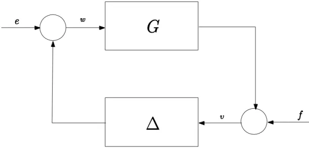
Figure 3. 1 Basic Feedback Configuration.

We consider systems of the form (3.8) where is a bounded and causal operator on .

(34)

20

(3.1) We often call the multiplier that defines the IQC. We will sometimes use the shorthand notation to mean that satisfies the IQC defined by . If , then can be taken as a transfer function satisfying

. The condition in (3.1) reduces to

(3.2)

Theorem 3.1 (Multiplier Theorem)[9]

Assume that

 The feedback interconnection of G and given in Figure 3.1 is well posed which means that is causally invertible since is linear.

 satisfies the IQC defined by

(3.3) where M can be factorized into where and their inverses are all causal and bounded

 There exists such that

(3.4) Then the interconnection of G and is stable.

If we compare the result in multiplier theorem with the corresponding result obtained in IQC stability theorem we see that the factorization condition is not needed in the IQC framework. The price paid for this is that well posedness is required for every feedback interconnection of G and , when .

The concept integral quadratic constraint (IQC) is used for several purposes:

 to exploit structural information about perturbations,

(35)

21

 to analyze combinations of several perturbations and external signals.

IQCs provide a way of representing relationships between processes envolving in a complex dynamical system, in a form that is convenient for analysis.

Depending on the particular application, various versions of IQC’s are available. Two signals and are said to satisfy the IQC defined by if

(3.5) where absolute integrability is assumed. Here, the Fourier transforms and represent the harmonic spectrum of the signals and at the frequency , and (3.1) describes the energy distribution in the spectrum of . In principle, can be any measurable Hermitian valued function. In most situations, however, it is sufficient to use rational functions that are bounded on the imaginary axis.

A time-domain form of (3.1) is

(3.6) where is a quadratic form, and is defined by

(3.7) where is a Hurwitz matrix. Intuitively, this state-space form IQC is a combination of a linear filter (3.7) and a “correlator” (3.6). For any bounded rational weighting function , (3.1) can be expressed in the form (3.6), (3.7) by first factorizing as

with , then defining

from and and M.

In system analysis, IQC’s are useful to describe relations between signals in a system component. For example, to describe the saturation , one can use the IQC defined by (3.1) with , which holds for any square summable signals

related by . In general, a bounded operator

is said to satisfy the IQC defined by if (3.1) holds for all

(36)

22

There is, however, an evident problem in using IQC’s in stability analysis. This is because both (3.1) and (3.6), (3.7) make sense only if the signals are square summable. If it is not known apriori that the system is stable, then the signals might not be square summable. This will be resolved as follows. First, the system is considered as depending on a parameter , such that stability is obvious for , while gives the system to be studied. Then, the IQC’s are used to show that as increases from zero to one, there can be no transition from stability to instability.

The feedback configuration, illustrated in Figure 3.1, is the basic object of study,

(3.8)

Here represent the “interconnection noise” and G and

are the two causal operators on and , respectively. It is assumed that G is a linear time-invariant operator with the transfer function in , and has bounded gain.

In applications, will be used to describe the “troublemaking” (nonlinear, time-varying, or uncertain) components of a system. The notation will either denote a linear operator or a rational transfer matrix, depending on the context. The following definitions will be convenient.

We say that the feedback interconnection of G and is well-posed if the map defined by (3.8) has a causal inverse on . The interconnection is stable if, in addition, the inverse is bounded, i.e., if there exists a constant such that

(3.9) for any and for any solution of (3.8).

When is linear, as it will be the case below, well-posedness means that is causally invertible. From boundedness of and , it also follows that the interconnection is stable if and only if is a bounded causal operator on

(37)

23

In most applications, well-posedness is equivalent to the existence, uniqueness, and continuability of solutions of the underlying differential equations and is relatively easy to verify. Regarding stability, it is often desirable to verify some kind of exponential stability. However, for general classes of ordinary differential equations, exponential stability is equivalent to the input/output stability introduced above.

Consider with . Assume that for any ,

the system

(3.10) has a solution . Then the following two conditions are equivalent.

 There exists a constant such that

(3.11) for any solution of (3.10) with .

 There exist such that

(3.12) for any solution of (3.10).

3.2 IQC Stability Analysis and Robust Performance Analysis 3.2.1 IQC Stability Analysis

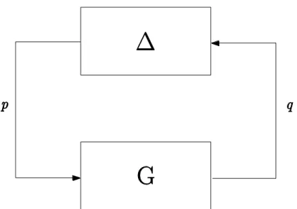
We start with the well-known condition for robust stability by means of IQCs for an unforced feedback configuration shown in Figure 3.2

(38)

24

Figure 3. 2 Robust analysis problem.

Theorem 3.2 (IQC Stability Theorem)[14]

Suppose is stable and

 The feedback interconnection of and is well-posed for all ,

 satisfies the IQC defined by for all . That is, for all ,

(3.13)

 satisfies

(3.14)

Then, the feedback interconnection of and is stable.

3.2.2 Robust Performance Analysis

Consider the system

(39)

25

Assume . We want to investigate if the closed loop system satisfies various performance objectives. The most common performance measure is the gain of the system. This corresponds to the IQC

(3.16) Assume . Then the system in (3.15) has robust performance with respect to the performance IQC if

 the system is stable

 for all .

To derive a condition for robust performance assume that we have the noise IQC (3.17) and the IQC

(3.18) for the uncertainty. We assume that has the block structure

(3.19) We can now give the following robust performance result.

Assume that satisfies (3.17) and satisfies (3.18). Then the system (3.15) has robust gain if

 it is stable

 the frequency domain inequality

(3.20)

holds for all .

3.2.3 The Kalman-Yakubovich-Popov Lemma

(40)

26

(3.21) is equivalent to a number of conditions on the system matrices in the realization of the transfer functions G and . The discrete time case can be treated similarly.

We will first derive an LQ optimal control formulation of (3.21). Let have the realization

(3.22)

where and is Hurwitz. Using (3.22) and

shows that (3.21) can be formulated as

(3.23) where

(3.24) and

(3.25) It follows that (3.23) is equivalent to existence of such that

(3.26)

for all pairs such that . This is

an LQ optimal control problem. The Kalman-Yakubovich-Popov (KYP) Lemma shows that (3.23) and the LQ optimal control problem above are equivalent to an LMI condition, a Riccati equation condition and an eigenvalue condition on the Hamiltonian matrix corresponding to the LQ problem.

Theorem 3.3

Assume the pair of matrices (A,B) is stabilizable and A has no eigenvalues on the imaginary axis. Then the following statements are equivalent:

(41)

27

 There exists such that for all pairs such that

(3.27)

 We have

(3.28)

 There exists such that

(3.29)

 , and the Riccati equation

(3.30) has a stabilizing solution , i.e., is Hurwitz.

 and the Hamiltonian matrix

(3.31) has no eigenvalues on the imaginary axis.

3.3 Representation of Time-Delay and Parametric Uncertainties via IQCs

which satisfies

(3.32) (3.33) where and are the functions defined by

(3.34) Note that (3.33) is just a sector inequality for the relation between and

(42)

28

As explained in [9], multiplying (3.32) by any rational function and integrating over the imaginary axis yields a set of delay-independent IQC conditions. In order to decrease the conservatism of the description and obtain a delay-dependent condition, one can multiply (3.33) by any nonnegative weighting function and integrate over the imaginary axis. Unfortunately, the resulting IQCs have nonrational weighting matrices . However, one can use a rational upper bound of and rational lower bounds and of and , respectively.

Then the point-wise inequality (3.33) holds with replaced by and with replaced by (the upper bound for the multiplier, the lower bound for the multiplier), respectively and can be integrated with a nonnegative rational weighting function to get rational IQCs utilizing delay bounds. With the inequality (3.33), the for time-delay uncertainty can be expressed as

(3.36) Instead of the multiplier given in (3.36), for a simpler identity which satisfies the previous sector inequality, a set of IQCs,

(3.37)

is used to define the time-delay operator where

is any nonnegative rational weighting function, and is any rational upper bound of

(3.38) For example, one can choose as

(3.39) Due to the multiplier theory, to be able to prove that (3.37) is sufficient enough to

define the time-delay operator one need to show

that satisfies

(43)

29

(3.40) When is replaced with and (3.37) is used for , then one can easily show that (3.40) is satisfied by the help of (3.37) and (3.38).

On the other hand, since the parametric uncertainty affecting the system matrices, is defined by multiplication with a real number of absolute value . Then it satisfies all IQC's defined by matrix functions of the form

(3.41)

where and are bounded and measurable

matrix functions. This IQC is the basis for standard upper bounds for structured singular values. [9]

in Figure 3.2 also involves the parametric uncertainties affecting the system matrices. From now on, will be described as where stands for the time delay on states, control inputs and derivatives of the states; describes the parametric uncertainty on the system matrices and .

Since has the block-diagonal structure and for satisfies the IQC defined by

(3.42) where the block structures are consistent with the size of and , respectively. Then, satisfies the IQC defined by

(3.43)

If, for is described by the cone , is described by . Addition and diagonal augmentation of any finite number of cones can be done in same way [40].

(44)

30

SECTION 4 FEEDFORWARD CONTROLLER SYNTHESIS VIA IQCs

In this section, the feedforward controller synthesis via dynamic IQCs is provided. The general problem is defined in the first subsection and the duality in multiplier theory is explained. The section is concluded with the theory of feedforward controller synthesis for uncertain time-delay systems.

4.1 General Problem Definition

Consider a class of time-delay system with stationary time-delay given as

(4.1) where real-time measurable states, initial conditions, and are constant time delays which satisfies , and

where , and are the known upper limits of delay, denotes the control inputs, is the disturbance vector acting on the system which is assumed to be restricted in a set of the form

(4.2) is an exogenous controlled output. Then , , , , , and are known real constant state-space system matrices of appropriate dimensions. The uncertainties and are matrix valued functions with appropriate dimensions.

(45)

31

4.2 Duality in Multiplier Theory

One needs to use the dual forms of the conditions involving the multiplier and G to carry out the feedforward controller synthesis. It can be shown that with , it can be assumed that . Due to (3.4), has the same number of negative eigenvalues as the number of inputs of G [41]. Since

, it can be shown that on .

Lemma 4.1 [14]

Let have full column-rank and be such that

. Then, iff where forms a basis for the

orthogonal complement of the image of S.

Lemma 4.2 [14]

Let be linear and suppose that is such that

on . Then, the following statements are equivalent, i.

ii.

Now by the help of these lemmas, one can define the equivalent condition for the dual form

(4.3) where

(4.4)

and deduce and on [15].

It is desirable to restrict to a subspace of and optimize over it. We wish to do this by specifying and optimizing over , where and

(46)

32

satisfies the IQC associated with . For several perturbation blocks, parameterization of a suitable multiplier (i.e. ) is available in the literature. However, since it is , and not , that appears linearly in our formulation, the structure of the inverse of the multiplier is paramount. The structures of some multipliers are inversion-invariant. An immediate example is multipliers of the form

(4.5) where is unstructured. Yet some structures are not inversion-invariant. In general, must be parameterized in a case-by-case manner. However, for linear blocks defined not only over but over , we can use the lemma and parameterize via the dual IQC,

(4.6) Hence, if s are known to satisfy the dual IQC, can be parameterized as , where . Alternatively, if s satisfy the primal IQC, one can take with . Based on a finite set of primal multipliers, this provides a generic recipe for constructing an affinely parameterized family of dual multipliers that is suited for our synthesis procedure.

4.3 Theory of Feedforward Controller Synthesis via Dynamic IQCs

can be decomposed as

(4.7) by using the minimal state-space realization

(4.8) For the decomposition of one can assume that is observable and

are Hurwitz. With the definitions of

(47)

33

one can reobtain (4.3) [14] as whereas has the realization of

(4.10)

On the other hand, can be defined as

(4.11) and for , one can apply the KYP Lemma to show that there exists an

such that

(4.12)

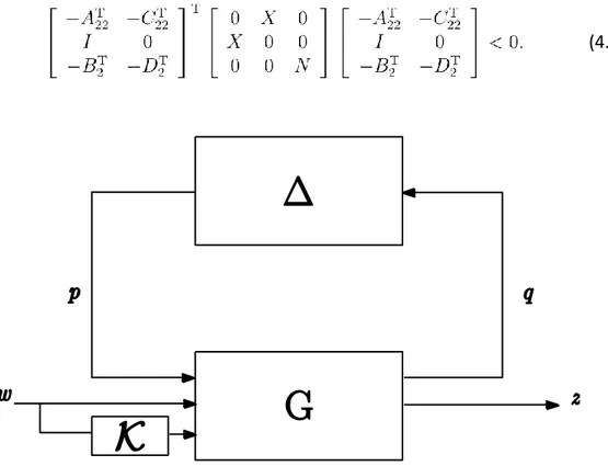
Figure 4. 3 Robust feedforward problem

Let us deal with the robust feedforward problem shown in Figure 4.3. The objective is to design a controller such that the closed-loop system has a minimum -norm from input to the output . We consider a plant with the state-space representation such as

(48)

34

where is Hurwitz. is realized as . Then, the nominal (delay-free) closed-loop system becomes

(4.14)

On the other hand, involving the multiplier realization, one can define

(4.15)

and with a suitable row partition with .

4.4 Feedforward Controller Synthesis for Time-delay Systems Having Parametric Uncertainties

A robust optimal stabilizing controller synthesis problem for nominal time-delay system (4.1) is considered so that the closed-loop system has minimum -gain, , which is defined as

(4.16)

Theorem 4.1

Given positive constants , the feedforward control law globally asymptotically stabilizes the system (4.1) with an

(49)

35

disturbance attenuation level of where the state, control and neutral delays are defined by the multiplier

(4.17) and the parametric uncertainty affecting the system matrices defined by the multiplier

(4.18)

if there exists matrices , , , and with

appropriate dimensions such that

(4.19)

(4.20)

where

(4.21) One can obtain the system matrices of dynamic controller such as

(50)

36

Proof: For the system with the time-delay and parametric uncertainty (4.1), dynamic

IQCs are used to represent the delay operator and parametric uncertainty. Then for the time-delay operator, using the multiplier allows to write

(4.23) Factorizing function in the multiplier leads to

(4.24) Then, by the help of the factorization we obtain

(4.25) As explained in the previous sections, we have two different multipliers for two different types of uncertainties which are delay operator and the parametric uncertainty. Since there are two multipliers, one needs to combine them and define a compact multiplier which consists of the two multipliers,

(4.26) and

(4.27) Here, (4.26) stands for the time-delay operator whereas the multiplier given in (4.27) stands for parametric uncertainty affecting the system matrices. As explained in Section 3.3, the combination of the two multipliers can be carried out and the final multiplier is given in the form of as follows

(51)

37

(4.28)

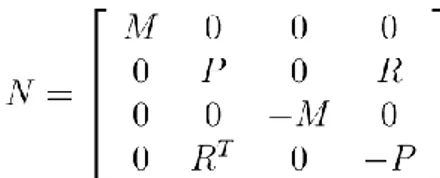
As explained in Section 4.2, by using the duality properties we have similar to the one in (4.4) which have the factorization in (4.7). So that we have the dual form of the total multiplier involving the time delay and parametric uncertainty in the form of where

(4.29)

and with [40]

(4.30) Suppose satisfies the IQC associated with which has the block-diagonal structure where and stand for the delay operator and parametric uncertainty, respectively. Then, the system has gain less than

is stable and

(4.31)

With the help of (4.15), one can obtain

(4.32)

(52)

38

(4.33)

Let us partition as

(4.34)

with nonsingular and . The congruence transformation is applied to (4.33)

(4.35)

and with the definitions of , ,

and , it leads to (4.20). On the other hand, it is needed to solve the LMI (4.19) because of the condition. Then, the closed-loop system is uniformly exponentially -stable if (4.21) holds which concludes the proof.

(53)

39

SECTION 5 NUMERICAL EXAMPLES AND SIMULATION STUDIES

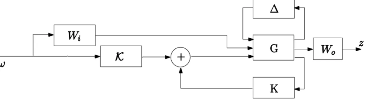
The results obtained by using the proposed controller synthesis, are illustrated by using different examples that can be classified into three groups: State and control delayed systems including an active suspension system, delayed systems with parametric uncertainties and neutral time-delay systems. All of the examples are the benchmark problems used in the literature for many times [42], [43], [44], [45], [46].

Figure 5. 4 Combined feedback and feedforward control scheme.

The examples are grouped into three case studies which involve state and control delay, time-delay and parametric uncertainty, neutral system (delay on state derivatives).

5.1 Case 1: State and Control Delay Example 5.1

Consider the following linear time-delay system.

(54)

40 where

(5.2) and are the upper bounds for the time delay that affect the states and control input of the system, respectively. An state-feedback controller whose gains are chosen as is employed to stabilize and control this system. Note that this feedback compensator is obtained from the well-known synthesis given in [47].

The aim of this study is to design a feedforward controller, , such that the closed-loop system is stable and has minimum gain, as an addition to the existing stabilizing feedback controller in a standard two-degrees of freedom control structure as shown in Figure 5.4.

Note that the disturbance is assumed to be measurable in this system. The multiplier is

assigned in the form of where and

which satisfies the dual of the IQC dealing with which here stands for the state and control input delay. Here we choose

(5.3) is also chosen as a second order Butterworth low-pass filter.

The cut-off frequency of this filter is chosen as where this filter is selected as (5.4) On the other hand, it is needed to choose as an approximate integrator which is

to eliminate steady-state errors.

We obtain the gains with changing order, which symbolizes the effect of the applied disturbances to the outputs of the system. Table 5.1 shows the obtained values of . Here, "FB" symbolizes the case of pure feedback control, whereas "FB+FF" stands for the combined feedback feedforward control scheme. Notice that the feedforward controller significantly reduces the gain of the closed-loop system