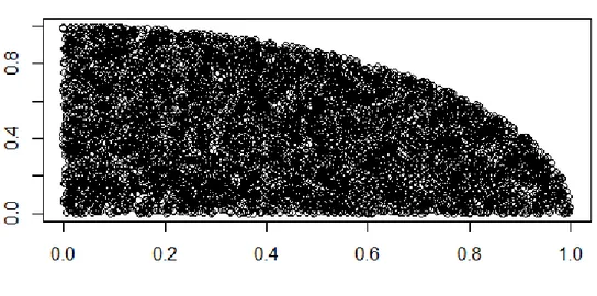
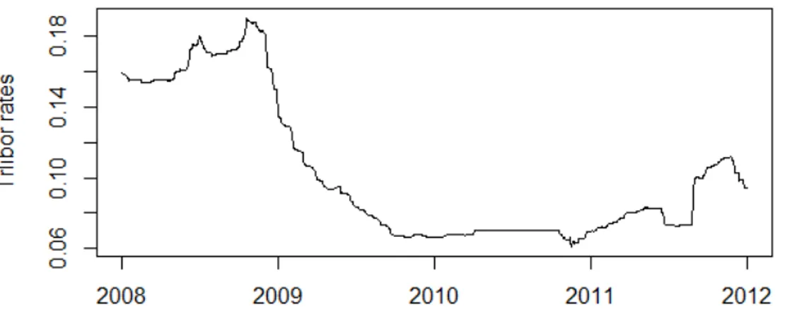
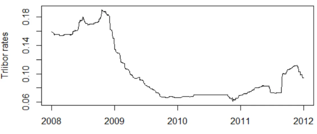
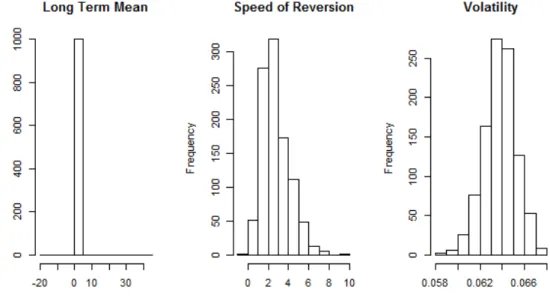
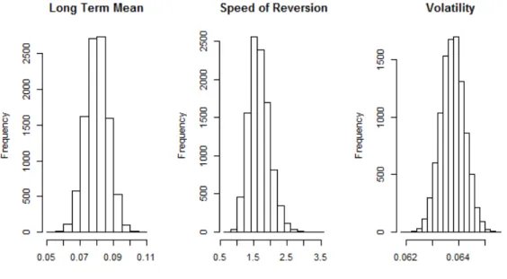
Distributions of the parameters in vasicek model

The aim of this study is to provide developing students’ awareness of mathematics in our lives, helping to connect with science and daily life, realizing

It was retrospectively evaluated whether there was a difference in the severity and course of stroke in acute ischemic stroke patients diagnosed with type-2 DM and taking

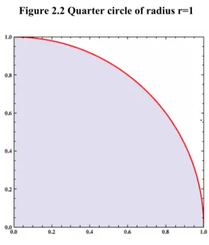
In this chapter we explore some of the applications of the definite integral by using it to compute areas between curves, volumes of solids, and the work done by a varying force....

Svetosavlje views the Serbian church not only as a link with medieval statehood, as does secular nationalism, but as a spiritual force that rises above history and society --

Therefore, the present study enriches the growing literature on meaning making and coping strategies of Chechen refugees by approaching the issue qualitatively: How

It shows us how the Kurdish issue put its mark on the different forms of remembering Armenians and on the different ways of making sense of the past in a place

One of the wagers of this study is to investigate the blueprint of two politico-aesthetic trends visible in the party’s hegemonic spatial practices: the nationalist

I also argue that in a context where the bodies of Kurds, particularly youth and children, constitute a site of struggle and are accessible to the