The effects of common macroeconomics factors on U.S stock returns

(1)

KADIR HAS UNIVERSITY

GRADUATE SCHOOL OF SOCIAL SCIENCES

THE EFFECTS OF COMMON MACROECONOMICS FACTORS ON U.S STOCK RETURNS

MASTER THESIS

SERKAN ŞENGÜL

(2)

SERKAN ŞENGÜL

Submitted to the Graduate School of Social Sciences in partial fulfillment of the requirements for the degree of Master of Arts in Economics

KADIR HAS UNIVERSITY Haziran, 2014

KADIR HAS UNIVERSITY

GRADUATE SCHOOL OF SOCIAL SCIENCES APPENDIX B

(3)

SERKAN ŞENGÜL

APPROVED BY:

Doç. Dr. K. Ali Akkemik (Advisor) Kadir Has Üniversitesi

Doç. Dr. Meltem Ucal Kadir Has Üniversitesi

Yrd. Doç. Dr. Arhan Ertan Kadir Has Üniversitesi

APPROVAL DATE: Haziran, 2014 APP

END IX C APPENDIX B

(4)

v

“I, SERKAN ŞENGÜL, confirm that the work presented in this thesis is my own. Where information has been derived from other sources, I confirm that this has been indicated in the.”

__________________________ SERKAN ŞENGÜL

(5)

vi

ABSTRACT

Common Macro Factors and Their Effects on U.S Stock Returns

SERKAN ŞENGÜL

Economics, Master Advisor: Doç. Dr. Ali Akkemik

Haziran, 2014

In this study, the macro variables’ explanatory power in relation to the variation of stock returns has been discussed in terms of the economy of the USA. In order to make an analysis on the cross section of the stock returns, 131 Macroeconomic variables between 1964 and 2007 have been put into use. Summing up the information in 131 monthly series, dynamic factor analysis is used to take out 8 potential factors. So that the pragmatic presentation of the factor model can be measured, Fama-Macbeth’s test procedure of two phases is applied. In addition to the variables included in the literature such as market risk factor, size factor, value factor and momentum factors, it is found out that the macro factors are highly influential on the explanation of the common variation in U.S stock returns. The tests stated above have been performed by the means of Fama French 49 industry portfolios, apart from Fama French 100 portfolios that have been formed on size and book. Furthermore, the factor model is established and intended for the certain periods of boom and recession. In comparison to the boom periods, the relations established between latent factors and stock returns appear to be unimportant during the downturn periods.

(6)

vii

ACKNOWLEDGE

First of all, I owe big thanks to my advisor, Doç. Dr. K. Ali Akkemik, for his help whenever I had trouble. He has more faith in me than I do. Special thanks go to my wife and my family for encouraging me in every tough situation and for their pure love. Lastly, I am grateful to TUBITAK for the generous support during master’s study.

(7)

viii

Table of Content

Abstract

Acknowledge

List of Table viii

List of Figure ix

Abbreviations x

1 Introduction 1

2 Literature Review 5

3 Methodology 17

3.1 Principal Component Analysis 17

3.2 Constructing the Factor Model 18

3.3 Determining the Factors 19

3.4 Two Stage Regression Procedure 21

4 Data and Factors 24

4.1 Information about the Data for Stock Return 24 4.2 Macro Series and Corresponding Factors 24

5 Results 33 6 Conclusion 45 References 48 Appendix 53 APP END IX C

(8)

ix

List of Table

Table 1 KMO and Bartlett’s Test ... 26

Table 2 Summary Statistics For Estimated Factors ... 27

Table 3 Time Series Regression of Individual Portfolios ... 34

Table 4 Time Series Regression of Industry Portfolios ... 36

Table 5 Time Series Regression of Individual Portfolios in Expansion Periods ... 37

Table 6 Time Series Regression of Individual Portfolios in Recession Periods ... 37

Table 7 Cross Sectional Regression of Individual Portfolios ... 39

Table 8 Cross Sectional Regression of Industry Portfolios ... 41

Table 9 Cross Sectional Regression of Individual Portfolios in Expansion Periods ... 42

Table 10 Cross Sectional Regression of Individual Portfolios in Recession Periods ... 43

Table 11 Comparison of Cross Sectional Regressions ... 44

Table A.1 Summary Statistics of Individual Portfolio ... 53

Table A.2 Summary Statistics of Industry Portfolios ... .56

Table A.3 Comparison of Expansion and Contraction Periods ... 58

Table A.4 Table A.4: The Description of 131 Monthly Macroeconomic Series ... 61 APP

END IX C

(9)

x

List of Figures

Figure 1 Marginal R-square for factor 1 ... 28

(10)

xi

Abbreviations

APT Arbitrage Pricing Theory

ARCH Autoregressive Conditional Heteroskedasticity ARDL Autoregressive Distributed Lag Model

ARIMA Autoregressive Integrated Moving Average BOT Balance of Trade

CAPM Capital Asset Pricing Theorem CPI Consumer Price Index

ISE Istanbul Stock Exchange KSE Karachi Stock Exchange MPT Modern Portfolio Theory PCA Principal Component Analysis PPI Producer Price Index

VAR Vector Autoregressive

(11)

1

1. INTRODUCTION

In the last few decades, a common wondering issue is the relationship between the economy and the financial sector (e.g. Chen et al, 1986; Cheung and Ng, 1998; Altay, 2003). The idea behind this curiosity is to find the effects of macroeconomic factors on the global financial crises. Although there are many works in the literature to investigate the relationship, so few have a close interest the interrelations between the macroeconomic factors and the financial variables. Moreover, the main difference of this study is to use 131 macroeconomic variables which are higher than all relative works.

According to many studies, there are significant effects of the macroeconomic factors such as inflation, interest rate, etc. on the stock returns (Fama, 1981; Chung and Tai, 1999; Christopher, et al., 2006). The most known model in order to analyze the interactions between the macroeconomic variables and the stock returns is the arbitrage pricing theory (APT). This theory was developed by Ross (1976) and asserts that various factors which created the risk factor can be used to explain the stock return. The first study with APT model in the literature was Gehr (1978). Such macroeconomic variables are used to explain the stock return in U.S. stock market (Chen et al, 1986). Their work was also the first empirical analysis of APT which is considered as a macroeconomic approach. They found that there are some variables such as the production or change in risk premiums which have positive effects, although some others such as the expected or unexpected inflation rate have adverse effects on the expected stock returns.

There are different models besides APT, such as Capital Asset Pricing Model (CAPM) or Modern Portfolio Theory (MPT) which show the relationship between the stock return and the macroeconomic factors. In addition, some authors designed their fact models according to the

(12)

2

purpose of the model. For instance, Fama and French (1992) included some microeconomic variables such as firm size or book to market equity to present the fundamental factor model. A different example can be seen in the study of Chen et al (1986). They included consumption and oil prices as macroeconomic variables to make an economic factor model. The APT can be considered as an extended version of the other models.

Bodurtha, Cho and Senbet (1989) expanded the study of Chen et al. (1986) by adding global factors to the model. First of all, they repeated the same analysis with the same macroeconomic factors and smaller sample data. However, the only significant factor is production of the industry. Then, they added five global factors besides the local factors and the expanded model yielded better results so that some insignificant factors became statistically significant.

By Martinez and Rubio (1989) or Poon and Taylor (1991), the relative studies were done for the UK and Spanish stocks market. They could not find any close relationship between the variables. Moreover, Gunsel and Cukur (2007) revised the study for the London Stock Exchange while Rjoub, Tursoy and Gunsel (2009) examined it for Istanbul Stock Exchange. In both studies, the researchers found that the variables have different impacts on the different individual and industry portfolios.

This paper examines how the macroeconomic variables work for explaining the cross section of the US share of earnings. It is put forward in the classical economic theory that the financial sector and the macro economy have common aspects. No single particular theory has prevailed in this study. Instead, various studies that associate asset prices and returns with macro variables have been used. When it comes to practice, making a decision on the

(13)

3

establishment of a corresponding link between the macro variables and asset prices becomes more difficult. The analysis covered in this thesis reveals an empirical attempt to establish and support this link.

To examine the cross section of stock returns, the papers written in this regard employed a limited number of variables. On the other hand, this paper presents 131 macroeconomic variables of the U.S. economy in relation to the dynamic factor analysis with the aim of extracting common macro factors. This leads to some advantages and disadvantages. Considering a large number of factors, it becomes obvious that certain errors related to measurement may not be that important compared to a few number of factors, because these factors will substantially vary. Besides, a single macro series may not be a priced factor while a combination of tens of them may be.

The punchline of this thesis is that when the latent macro factors are reverted on Fama French 100 portfolios that are based on size and book, they turn into substantially priced risk factors. In addition, some of those potential macro factors come up with a great capacity of providing explanation far beyond the CAPM, Fama French 3 factor model and adding the momentum factor to the Fama French. Furthermore, the research has been conducted with various kinds of portfolio structures, referring to 49 industry portfolios to ensure reliability. Another identified aspect relates to the efficiency of some latent factors in explaining the common movement of industry portfolios. Finally, some tests have been applied separately to expansion and contraction periods. On the one hand, the factors that have been taken out could not account for the priced risk factors in recession periods. On the other hand, some of the latent factors appeared to be unimportant in expansion periods.

(14)

4

In the second part of this thesis, a literature review compares various studies and methodologies that have been used. Part 3 describes the methodology in detail. Part 4 explains the data set and the macroeconomic factors. In the fifth part, the results are discussed in conjunction with the methodological aspects. The final part, 6, wraps up and concludes the thesis.

(15)

5

2. LITERATURE REVIEW

Examining the relationship between risk and return is required the factor models. Furthermore, there is an allegation on their part regarding that the systematic risk is completely under the control of the factors. What the factors that have been set out in a factor model explain is about the reason why some group of stocks’ returns is inclined to act together. Also they are needed to explain the variations of the stock returns in details.

The two most widely used and popular theories in relation to the asset pricing literature are the Capital Asset Pricing Model (CAPM) and the Arbitrage Pricing Theory (APT). In the CAPM, systematic risk is the unique factor to explain the variations of the stock returns. As it gets larger, the return is expected to increase to the same extent. Regarding this, the CAPM brings up the idea that there is a linear relationship between the expected return and the systematic risk.

The model was constructed and introduced by Jack Treynor (1961), William Sharpe (1964), John Lintner (1965) and Jan Mossin (1966) independently, and it is mostly based on the previous works conducted by Harry Markowitz’s Modern Portfolio Theory (MPT), drawn up in 1950’s. The CAPM is deemed valid along with the following assumptions:

 Investors come to agreement about the return distribution

 Investment horizon is fixed for each investor

 Investors make use of the efficient portfolios that establish a connection between the CAPM and MPT

 Borrow and lending can be done at risk free rates

 There is an equilibrium in the stock market

(16)

6  There is a perfect information

The experimental studies conducted by Gibbons (1982), Reinganum (1981), and Coggin and Hunter (1985) all point out that the CAPM does not work efficiently. To compensate the drawbacks of the CAPM model, Ross (1976) developed the Arbitrage Pricing Theory (APT). The APT offers predictions on the relationship between an asset return and risk premiums the different factors. Reflecting the differences between the theories included in this study so far, the APT does not put forward equilibrium unlike the CAPM. The CAPM can be regarded as a special case within the scope of the APT. Therefore, it actually does not determine the factors. Moreover, the APT comes up with softer presumptions as follows:

 A factor model is able to describe all common variations

 No arbitrage opportunities are available.

 The idiosyncratic risk can be diversifiable.

The factors are required for the APT. Since they are not set out in the theory, some models or analysis techniques are required to extract the factors. In the macroeconomic models, there is a comparison between stock returns and the macroeconomic variables such as the interest rate, inflation, or production. Certain macroeconomic factors have been used by Chen, Roll and Ross (1986) to provide an explanation for the stock returns.

The second way to extract the factors is econometric models. The most known type of econometric model in this sense is the Principal Component Analysis which is explained in the methodology section.

(17)

7

Another method is data mining which enables determining the correct portfolios, the returns of which can be proxy variables for the factors. Fama & French state that there are two factors which are value and size besides the systematic risk and these factors have great explanatory power for the stock returns. Post and Levy (2005) found that the firms which have small market capitalization (counted as small firms) have positive abnormal returns around 2-4% per year while larger firms with have large market capitalization have negative abnormal returns. Post and Levy (2005) concluded a result about the value effect that value stock has positive abnormal returns approximately 4 and 6 percent a year. This model of Fama and French was extended by Carhart (1997) who adds a momentum factor. Post and Levy (2005) state that the momentum effect is more important than size and value effect so that it has a significant effect in determining the stock returns. Especially for small firms which are categorized according to the size factor, the momentum effect became more significant.

Chan, Chen and Hsieh (1985) investigated the size effect on the stock return for small number of firms which have high average return and different size. They constructed a data set for 20 firms and their macroeconomic factors were growth of the production, change in risk premium, inflation, etc. They took the difference between two portfolios which are the smallest and the biggest to determine which factors are important. They found that the change in risk premium is the most deterministic factor for the stock returns of the firms which have different sizes.

Roll and Ross (1980) extended the first research, which was done by Gehr (1987), by enlarging the data set in order to find the significance of the test for the stock returns. They examined using this factor model the New York Stock Exchange between 1962 and 1972. They concluded that the test which was made for the five factors model produced the weak

(18)

8

results for the expected stock returns. In 1984, Dhrymes, Friend and Gultekin tried to identify the problems in the analysis of Roll and Ross (1980). The first one is that the number of risk factors which were identified was increased with the number of securities proportionately. The other one is that there was a complication about diagnosing the factors that generate the stock returns.

Some information about the study of Chen, Roll and Ross (1986) were given before but some more details should be discussed in this section since their work is the closest one to this study. They decided to use a different factor model which contains macroeconomic variables (in the 1980s), in order to find the significant factors for the asset returns. They used the Fama-Macbeth two pass regression model to forecast the relationship between the macroeconomic variables and the stock returns. Their main purpose was to find firstly the estimated risk premium for every factor used in the model and then to conduct a test to check their significance. They obtained that four of the factors, risk premium, industry production, interest rate and unexpected inflation, have mixed significance effects to explain the stock returns.

Poon and Taylor (1991) used the same model with Chen et al. (1986) in order to determine the stock returns for UK stock market. However, unlike Chen et al. (1986), they could not find any significant effect of the macroeconomic factors on the stock returns. Martinez and Rubio (1989) repeated the same exercise for the Spanish stock market; but they could not either obtain any meaningful relationship between the stock returns and the used factors. On the other hand, Hamao (1988) examined the same framework for the Japanese stock market and according to his study, anticipated inflation, risk premium and interest rate have significant effects on the stock returns.

(19)

9

Cauchie, Hoesli and Isakov (2003) studied the effects of macroeconomic variables on the returns of stocks which were taken from Swiss stock market by using the APT model. They extracted the macroeconomic factors via the principal component analysis and the significance of four variables for stock returns was confirmed by using 17-year monthly data. Gunsel and Cukur (2007) used a portfolio model to explain the stock returns for London Stock Exchange and they found that all independent variables, which are eight macroeconomic variables, have significant effects on the stock returns.

Most economists have examined on the effects of macro-economic variables such as interest rate, inflation, exchange rates, money supply, etc., on the stock prices and investment decisions over the last decades. Thus, theoretical and empirical literature has been used as the most efficient way to be able to analyze the relationship between stock returns and economic forces at the macro level. According to Saeed and Akhter (2012), the theoretical and empirical literature review has enabled the researcher to know the work done in the subject area by other researchers and to identify the macro-economic factors that can potentially influence the returns of stocks. The empirical evidence in the literature facilitates an evaluation of the validity of the relationship between macro-economic forces and stock returns. Nevertheless, the direction of causality is still muddy both in theory and empirics (Aydemir and Demirhan, 2009).

Priyanka and Kumar (2012) argued that the external sector indicators such as the exchange rate, foreign exchange reserves and the value of trade balance might affect the stock prices. They used monthly data from 1994 to 2011, and mentioned that the exchange rate, gold price and the inflation rate had significant effects on the Indian Capital Market. According to Fisher (1930), there was a positive relationship between inflation and stock returns because of the

(20)

10

fact that as the rate of inflation raised, the nominal rate of interest increased. Consequently, the real rate of interest did not change in the long-run.

In order to examine the long and short run relationships between Lahore Stock Exchange and macro-economic variables in Pakistan, Sohail and Hussain (2009) used monthly data from December 2002 to June 2008. They found out that the consumer price index had a negative influence on the stock returns. On the other hand, the industrial production index, the real effective exchange rate, and money supply had larger positive effects on stock returns in the long-run.

The relationship between macro-economic indicators and the stated variables in Turkey were examined by Aydemir and Demirhan (2009) who used daily data from 23 February 2001 to 11 January 2008. They applied three different indices, namely, stock prices, national 100 index, services, financials, industrials, and technology indices. They found out that there was a bidirectional causal relationship between the exchange rate and all stock market indices. Negative causal relationship was found from national 100 index, services, financials and industrials indices to exchange rate. Also, they determined the negative causal relationship from the exchange rate to all stock market indices. Also, there was a positive causal relationship from technology indices to the exchange rate.

Using ARIMA model and quarterly data from the period 1986-2008, Mohammad et al. (2009) established the relation between share prices of KSE (Karachi Stock Exchange) and foreign exchange reserves, the exchange rate, the industrial production index, the whole sale price index, gross fixed capital formation and broad money in Pakistan. They found out that the foreign exchange rate and foreign exchange reserves affected the stock prices significantly

(21)

11

after the reforms in 1991. While external factors like money supply and the foreign exchange rate affected prices in a positive way, other variables like the whole sale price index and gross fixed capital formation had an insignificant influence on stock prices insignificantly.

Yusof et al. (2006) examined the long run relationship between macro-economic variables and stock returns in Malaysia by using the autoregressive distributed lag model (ARDL) and diverse macro-economic variables such as the money supply, Treasury bill rates, the real effective exchange rate, and industrial production index. They found that the money supply was positively related with the changes in stock prices while exchange rate had a negative effect on stock prices in the Malaysian market.

By using Granger causality test, Khalid (2012) explained the unidirectional causality from the exchange rate to stock performance on the Karachi Stock Exchange (KSE) return. Additionally, Dasgupta (2012) used the co-integration test and found out that the Indian stock markets are co-integrated with macro-economic variables. In the long-run, the stock prices were found to be positively related to the interest rate and industrial production. However, the whole sale price index used as a proxy for inflation and the exchange rate were negatively related to Indian stock market returns. But, those findings failed to establish short-run relationships between the Indian stock market and macro-economic variables.

Adam and Tweneboah (2008) investigated the existence of a long-run relationship between macro-economic variables and the stock prices in the studies about Ghana. They argued that inflation and exchange rates were significant determinants of share prices in the short-run while the interest rate and inflation were more important in the long-run.

(22)

12

Kuwornu and Owusu - Nantwi (2011) used the maximum likelihood procedure and investigated the relationship between stock returns and macro-economic variables such as the inflation rate, the exchange rate and Treasury bill rate. They demonstrated that inflation had a positive relationship with stock return while the exchange rate and Treasury bill rate had a negative impact on stock returns. However, there was no significant relationship between stock returns and crude oil prices.

In addition, Kuwornu (2012) found using the Vector Error Correction approach out that in the long run stock returns were positively affected by inflation, the exchange rate and Treasury bill rate and negatively by crude oil prices. They attribute variations in stock returns to inflation by a negative effect and Treasury bill rate by a positive effect in the short run.

Mahmood and Dinniah (2009) analyzed various causal relationships between foreign exchange rate, CPI, industrial production index and stock prices in Japan, Malaysia, Hong Kong, Thailand, Korea, and Australia. They used Error Correction Model using monthly data from January 1993 to December 2002. They concluded that there was a long run equilibrium relationship between these variables only in four countries; Japan, Korea, Australia and Hong Kong and only in the short run. Furthermore, there was no interaction in the short run relation between the above mentioned variables in all selected countries except between real output and stock prices in Thailand and between the foreign exchange rates and stock prices in Hong Kong.

By using a standard discounted value model and co-integration analysis, Humpe and Macmillan (2009) examined whether industrial production, CPI, long run interest rate and money supply influence to the stock prices in Japan and the U.S. They found out that the data

(23)

13

were consistent with a single co-integrating vector, where stock price was negatively related to CPI and long run interest rate but positively related to industrial production in the U.S. Also, there was a positive but insignificant relationship between the U.S. stock prices and money supply. In addition, they found two co-integrating vectors for the Japanese data. Stock prices were positively influenced by industrial production and negatively by the money supply. But the consumer price index and long-term interest rates negatively influenced the industrial production.

The relationship between various macro-economic variables and stock market prices in Pakistan was examined by Ali et al (2010) who applied the method of Johansen’s co-integration and Granger’s Causality Test using data from June 1990 to December 2008. They used the inflation rate, balances of trade, the exchange rate, and the industrial production index as macro-economic indicators. According to them, there was no causal relationship between macro-economic variables and stock exchange prices, but there was co-integration between the industrial production index and stock exchange prices. They added that performance of macro-economic variables could not predict stock exchange prices and stock market prices did not reflect the macro-economic condition in Pakistan.

Akay and Nargeleçekenler (2009) studied the relationship between monetary policy, the interest rates and stock prices using a Structural VAR (SVAR) model, and considering the inflation rate and industrial production index. They showed that a contractionary monetary shock was influential on the interest rate in both long and short run. But, it affected the stock prices negatively.

(24)

14

Gencturk (2009) studied the relations between stock prices in Istanbul Stock Exchange (ISE) and macro-economic variables in normal periods and crisis periods. While he took ISE-100 index as the dependent variable; he took Treasury bond interest rates, consumer price index, money supply, industrial production index, the exchange rate and gold prices as independent variables.

In addition, Sayılgan and Süslü (2011) examined the impact of macro-economic factors on stock returns in emerging market economies using panel data from 1996 to 2006. Stock returns were significantly influenced by the exchange rates, inflation rate and the S&P 500 Index. However, interest rate, money supply, gross domestic product, and oil prices did not affect the stock returns.

Aktas (2011) studied the influence of 19 macro-economic announcements on equity index options in ISE for the period from 1983 to 2002. According to her, seven macro-economic announcement series, namely, BOT, PPI, CPI, housing starts, money supply, retail sales and employment had significant effects on the option returns and volatility. Also, the balance of trade, producer price index, consumer price index, money supply, employment, retail sales and housing starts were strongly related with index option returns.

Huang and Chen (2011) investigated the interactions among stock returns, the term structure of interest rates and economic activities in Taiwan using various time series techniques including VAR, Granger Causality Test, Impulse Response Function and Variance Decomposition. They found causality between stock returns and industrial production and between stock returns and the spread in the long-term and short-term interest rates. However, they did not observe causality between the spread and industrial production. And the

(25)

15

industrial production could not respond to the spread obviously in the long-term and short-term. The term structure of interest rates was not influential on economic activities in Taiwan.

Hosseini et al. (2011) studied the relationship between stock market indices and four macro-economic variables including crude oil price, money supply, industrial production and inflation rate in China and India for the period from January 1999 to January 2009. They found out that there were both long and short run linkages between macro-economic variables and stock market index in both countries.

The relationships between various macro-economic variables, sectorial indices and the stock market index for the short run and long run equilibrium in Singapore were explained by Maysami et al. (2004). They showed that Singapore stock market and property index could be easily cointegrated with the changes in interest rates in the short run and long run, industrial production, price level, the exchange rate and money supply.

Gunasekarage et al. (2004), who studied on the equity values of the money supply, consumer price index, Treasury bill rate, the exchange rate in stock market in Sri Lanka, used the co-integration and vector error correction model using monthly data between 1985 and 2001. They reached out that macro-economic factors had a significant effect on the stock market.

In order to explain the influence of the U.S. stock prices on the Saudi local stock market returns, Alshogeathri (2011) evaluated the relationship between eight macro-economic variables, namely, two different measures of money supply, short-term interest rates, consumer price index, the size of bank credits, world crude oil prices, the exchange rate and the S&P 500 index. He used various vector auto regression and autoregressive conditional

(26)

16

heteroskedasticity model to analyze monthly data from 1993 to 2009 in the long run and short run. As a result, he found that the Saudi stock price index and money supply, short run interest rate, inflation and the U.S. stock market had a positive relationship in the long run. However, Saudi stock market returns, money supply and inflation had significant unidirectional causal relationship in the short run.

The influence of macro-economic factors on Amman stock market returns were examined by El-Nader and Alraimony (2012). They used monthly data from 1991 to 2010. According to the results of the ARCH (1) estimations, real gross domestic product had a positive effect, whereas real money supply, the real exchange rate, consumer price index, weighted average interest rates on loans and advances had a negative rimpact on Amman stock exchange returns.

(27)

17

3. METHODOLOGY

In this section, first the principal component analysis and then the method of research for asset pricing will be explained. The determined latent factors will be extracted using the principal component analysis. In addition, two-stage Fama Macbeth regressions of latent factor portfolios will be employed.

3.1. Factor Extraction

There are numerous factor extraction methods such as maximum likelihood method, principal axis factoring, principal component analysis, alpha method, unweighted lease squares method, generalized least square method and image factoring. However, the most commonly used method to extract the factors is the Principal Component Analysis.

The main advantage of this method is that linear combinations of the observed variables can be created. The first extracted factor is a combination that accounts for the largest variance in the sample and the second extracted factor accounts for the next largest variance while making it uncorrelated with the first. This process goes on until the last factor. Hence, all extracted factors have a power to explain the portions of total variance, and they are all uncorrelated with each other (Maracuilo and Serlin, 1988).

Principal Component Analysis (PCA) is a model used to find correlations of the data. The PCA sets out the use of principal components which are reduced as its main objective to indicate the original variables.

The principal component analysis functions for resolving the problems related to the measurement error in data series. This analysis expects a great number of macro series to be explained by a few potential factors. Stock & Watson (2002) and Bai & Ng (2002) pointed

(28)

18

out that the PCA can be used to extract the latent factors. Stock and Watson (2006) employed the analysis in different estimation methods and discussed its certain advantages and disadvantages. They seek to make a comparison between the performances of estimation methods for the industrial production in the U.S. To convey their statement in this regard, they argued as follows: “the dynamic factor analysis allows us to turn dimensionality from a curse into a blessing”. Ludvigson and Ng (2007) also employed the model to take factors out in order to explain the excess return in the stock market.

As stated above, the PCA is a common method to make a prediction about the factors. This thesis utilizes this model to determine the potential factors and then to test their significance.

3.2. Constructing the Factor Model

According to the literature review, the following equation for , is most appropriate in return

time t.

; E( ) = 0; cov( ) = 0 (1)

where,

 : actual return

 : constant term or intercept  : slope coefficient

 : factor

 : error term

After adding the basic econometric assumptions that the error terms are not correlated with each other (cov( ) = 0) in order to get rid of the autocorrelation problem, the model

(29)

19

the return of an asset are not correlated with each other. The final assumption about the equation (1) is that the residuals are not correlated with the independent variables.

After constructing the factor model, all factors should be derived specifically. Three different strategies in the literature can be used to determine the factors. These three methods, using the economic variables, econometric models and data mining, are discussed in the literature review section.

3.3. Determining the Factors

Using macroeconomic variables is very useful in examining the variation in the U.S. stock returns. In this direction, the variable, , is added to the model to denote all macroeconomic variables. Implied factor model may result in some measurement errors because the data used is very large. To get rid of the problems, needs to be defined as a specific regression

model as follows:

and (2)

(3)

where,

 represents r x 1 latent factors

 Ʌ represents N x r factor loadings

 represents N x 1 residuals

To show the consistency of the factors, consider two conditions1;

- is an N dimensional data vector and where D is r x r matrix with full rank. The limit is taken as N ∞ so that the factors can affect most of the series and the factor loadings are derived from different series, i.e. they are not homogenous.

1

(30)

20

- maxeval( ) ≤ c ≤ ∞ for all N where maxeval represents the maximum eigenvalue and . With this condition, the idiosyncratic terms have limits in the correlation with series (Chamberlain and Rothschild, 1983). Ludvingson and Ng (2009) used different notation to show the limitations of the contributions of the idiosyncratic covariance to total variance.

The estimators of derived as the weighted average of by using N x r matrix, W= (eigenvector matrix derived by the sample variance matrix of ) which is normalized by and . If as N ∞ where H is r x r matrix with full rank. Also, if the two conditions above hold then the estimated latent factors are consistent, which can be shown as follows:

_{as N  ∞ because} _{by assumption and because} _{by the weak law of large numbers.}

The least square problem is solved to derive the latent factors by the principal component analysis;

where (4)

After minimizing the above equation, will be the first r principal components of .

Consistency of the estimated extracted factors for finite T and N∞ was first shown by Connor and Korajczyk (1986). Stock and Watson (2002) showed that the consistency of the

(31)

21

estimated factors can be obtained because the residuals in this estimation do not affect the OLS coefficients.

3.4. Two Stage Regression Procedure

The next step, after the construction of the factor model, is the evaluation of the performances of the factors. The best way to measure the performance in APT is Fama-MacBeth model. Fama-MacBeth (1973) is a commonly used method in order to determine the estimated values of APT variables. The process has two stages. The first one is a time regression. In this regression, the estimated slope coefficients are determined and then they are used to realize the second step of the regression in order to measure the risk premiums.

To estimate the slope coefficients, the following regression model is used.

(5)

(6)

In the regression model above, the risk factors are represented by the latent macroeconomic factors. The regressions will be repeated by adding the market risk factor, size, value and momentum factors.

 Combining the latent factors and the market risk factor gives the following equation:

(7)

(32)

22

 Adding the size & value factor to the existed factors gives the following equation:

(9)

(10)

 Finally, inclusion of the momentum factors to the above regression equation gives the following:

(11)

(12)

o : market risk factor

o : market return

o : risk free rate

o : size factor is o : value factor

o : momentum factor o : size risk premium o : value risk premium o : momentum risk premium

The second stage of the regression is the estimation of the factor premiums with the following regression equation for just latent factors where lambda shows the risk premium factor.

(13)

(33)

23

All portfolio returns are regressed separately in each period on the estimated betas that are found in the first stage in order to examine the risk premiums. The above equation will be revised by adding the factors which are same before analyzing their effects.

The following equation shows the inclusion of CAPM into the previous one.

(14)

The following equation shows the inclusion of size and value factors to the previous one.

(15)

The following equation shows the inclusion of momentum factors to the previous one.

(16)

where the hat sign represents the estimated coefficients.

The null hypothesis of the test for the lambdas is that the average of the lambdas for each factor are equal to zero against the alternative hypothesis that it is significantly different from zero .

(34)

24

4. DATA AND FACTORS

4.1 Information about the Data for Stock Return

Kenneth R. French’s website provides access to Fama French Data Library, from where the data on stock returns and supplementary factors were obtained. Two different data sets are used for the stock returns: The first one is 100 portfolios formed on size and book and the second one is 49 industry portfolios. In testing the constructed factor model, using portfolios rather than individual shares has more benefits. The betas obtained using the portfolios is less tedious than individual shares which make Fama-Macbeth test model more efficient in relation with the downturns. The two different sets of data are, per month, value-based, limited to the timeframe during 1964 - 2007. Summary statistics are represented in table A.1 and A.2 in the appendix.

As stated before, the factor model is formed for boom and recession periods. The web site of NBER is the provider of the data about the periods. It is possible to observe higher average returns of growth periods when portfolio statistics of growth and recession periods are compared, and this is an expected result. Furthermore, in recession periods, there are larger standard errors for the stock returns. This can be shown as a proof to the asymmetric volatility. In order to find the comparison table of growth and downturn times, it is possible to look at appendix table A.3.

4.2. Macro Series and Corresponding Factors

Ludvingson provides a large data set about macro series between the desired dates in his website2. The same data was used in the analysis of Ludvingson and Ng (2009b). The main purpose of using this set of data is to examine the relationship between the macro series and

2

(35)

25

the excess bond returns. Furthermore, Stock and Watson (2005) used almost same data as in Ludvingson and Ng (2009a) to analyze the effects of macro series on the bond yields. There is just one macro variable in Stock and Watson (2005) which was not used in and Ludvingson and Ng (2009a) because there is no data about this macro factor in the dates which are used in their study. Different standardization methods were used for all series to promote stationarity. The standard normalization technique was used in this study before implying the PCA. The general procedure and the assumptions of the PCA were stated in the methodology section, and in this thesis I used the same macroeconomic series as Ludvingson and Ng (2009a). All assumptions hold and the procedure can be applied.

Before extracting the latent factors by PCA, the Bartlett Test of Sphericity and the Kaiser-Meyer-Olkin (KMO) measure of sampling adequacy should be applied. Bartlett Test of Sphericity is required to determine whether the correlation matrix is an identity matrix. If the test results for sphericity is large and the related level of significance is small, it means that the population correlation matrix is an identity matrix. Subsequently, a factor model should be considered to analyze the model.

The Kaiser-Meyer-Olkin (KMO) measure of sampling adequacy test is used to determine whether the sample is suitable for a factor model or not. It compares the magnitude of the observed correlation coefficients to the magnitude of the partial correlation coefficients. The interpretation of the test statistics is similar to the coefficient of determination. The closer the KMO measure to 1 the more suitable the sample for a factor model. Values smaller than 0.5 (closer to 0) mean a factor analysis of the variables may not be a good idea.

(36)

26 Table 1. KMO and Bartlett’s Test

Kaiser-Meyer-Olkin (KMO) Measure of Sampling Adequacy 0.818

Bartlett's Test of Sphericity Chi-Squared 3461.178

Degrees of Freedom 8515

Sig. .000

The KMO value is 0.818, which is higher than 0.5, so it is confirmed that there is a correlation among the macroeconomic variables (see Table 1). Hence, the factor analysis, the principal component analysis to extract the latent factors can be used. Besides, the Bartlett’s Test of Sphericity proves the adequacy of the PCA for macroeconomic variables.

The 131 macroeconomic series used in this thesis are gathered into eight groups. All series are listed in table A.4 in the appendix. These groups are as follows:

1. “Output and Income” (1-20)

2. “Labor Market” (21-50 and 129-131) 3. “Housing” (51-60)

4. “Consumption” (3-5 and 61-70) 5. “Money and Credit” (71-81)

6. “Bond and Exchange rates” (86-107) 7. “Prices” (108-128)

(37)

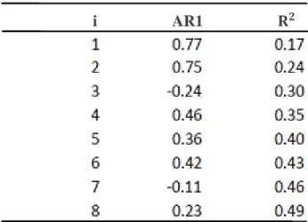
27 Table 2:Summary Statistics for Estimated Factors

Table 2 shows the correlation of the factors with the macro data series. AR1 column shows that there is much fluctuation among the factors. In other words, the factors are not fixed separately, they change from -0.24 to 0.77. R square shows the degree of total variations that can be explained by the independent variables. With this result, all factors altogether have 49% explanatory power. The table shows that the first factor discloses the most important one because it alone can explain %17 of the total variation. The second one and the rest have lower importance because their explanatory power decreases.

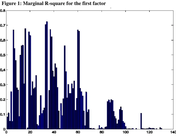
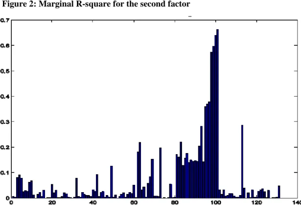
It is highly difficult to determine the factors specifically and to interpret their meaning economically because these factors come from different macroeconomic series. However, it is possible to show the relationship between the estimated factors and the macroeconomic series looking at the Marginal R squares for all factors. This feature of the factors can be examined by using regression model with the estimated factors as independent variables. In Figure 1, first factor is determined by mostly first, the second and the third groups. According to Figure 2, the second factor is related to the sixth and eighth groups. In the Figure, 3, the corresponding factors are related with price, i.e., the seventh group. Figure 4 shows that factor

(38)

28

4 is related with the first, second, third, sixth and seventh. In Figures 5 and 6, the corresponding factors 5 and 6 are related to each group, so it is so difficult to make any specific interpretations about these factors. According to Figure 7, the factor depends on the fifth group while the final factor in the last figure (Figure 8) is based on the eighth group, which is the stock market.

(39)

29 Figure 2: Marginal R-square for the second factor

(40)

30 Figure 4: Marginal R-square for the fourth factor

(41)

31 Figure 6: Marginal R-square for the sixth factor

(42)

32 Figure 8: Marginal R-square for the eighth factor

(43)

33

5. RESULTS

In model construction, it is necessary to determine the factors which are useful besides the eight factors. CAPM coefficient (market risk factor), Fama French coefficients (size, value) and momentum factor will be added to the basic model to show the differences between models.

 The first model is constructed with only 8 latent factors to find whether there is a relationship between these factors and stock returns.

 The second model is constructed with 8 latent factors and CAPM coefficient to show whether the explanatory power of the latent factors increases with the market risk factor.

 The third model is constructed with 8 latent factors and Fama French 3 factors. It is used to show the changes in the model when size and value factors are added to the model. Specifically, the changes in the significance of the latent factors will be investigated.

 The final model is constructed by adding the momentum factor to the previous model to investigate the effects of this factor on the explanatory power of the latent factors.

In the regression analyses of these four different models, Fama MacBeth two stage regression is used. In this method, four different data are employed to show the differences between models. Individual portfolios (100 units), industrial portfolios (49 units) and the recession & boom periods of the individual portfolios are used to estimate the regression.

(44)

34

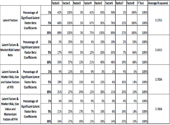
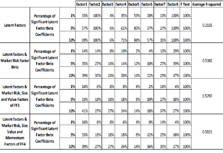
Table 3.Time Series Regression of Individual Portfolios

It is possible to see the beta parameter assessments of risk factors for individual portfolios in Table 3. The table also indicates the rate of portfolios that include significant beta estimation. F test demonstrates the importance of the regression formula in general sense. In conclusion, the table reveals the average levels of the R squared. Examining the F significance levels, it is observed that 100% of the time series regressions have substantial F test at three different critical levels.

Moreover, we can deduce from the table that the inclusion of the factor for market risk with eight latent factors results in a substantial increase from 0.276 to 0.643 in the average R

(45)

35

squared. Adding the Fama French factors (size and value) increase the R squared. Inclusion of the momentum factor as a final one leads to a small raise in the explained part of the total variation.

Furthermore, in the first regression model which is constructed with only latent factors, two of them do not appear significant, namely, factor 3 (price) and 7 (money and credit). The interpretation of this insignificancy is that the macro series about the price and money and credit have no effect on the individual portfolios. On the other hand, the stock market (the eighth factor) and the labour market (the second factor) have the largest significance level in all models.

In conclusion, without taking the insignificant factors (3 and 7) into consideration, the explanatory power of the factors has fallen by adding the extra factors, CAPM coefficient, size and value and momentum factor although the average R squared of the regression models have increased.

(46)

36

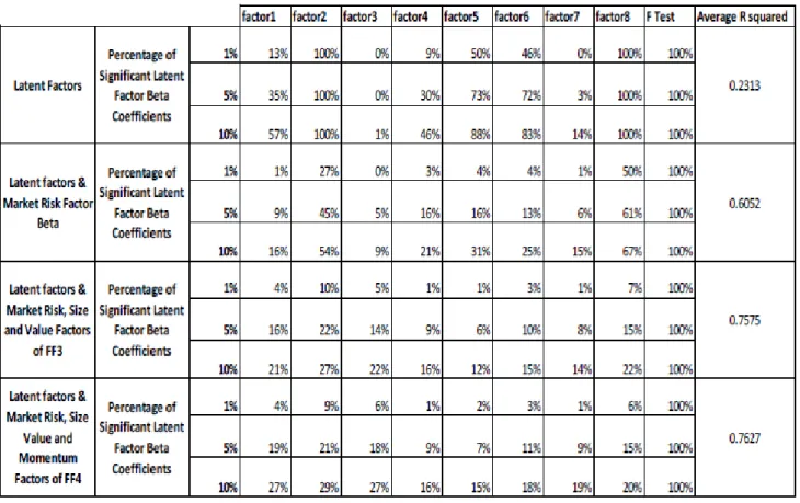
Table 4. Time Series Regression of Industry Portfolios

In Table 4, the regression results of the estimated beta for industry portfolios are shown. According to the results, F statistic is significant for the industry portfolios. Moreover, average R squared has an increasing trend, rising with the number of the explanatory variables. The average R squared can give an idea about the comparison between two factor models which are with individual and industrial portfolios which have lower value. There is no change in the care of the third and seventh factors, but the significance level of the other factors is higher in this model than the previous one. However, their significance levels have a decreasing trend when expanding the model with additional factors.

(47)

37

Table 5. Time Series Regression of Individual Portfolios in Expansion Periods

(48)

38

To clarify the difference between thebehavior of stock returns in boom and recession periods, two factor models are implemented. The results of time series regression for boom and recession periods of individual portfolios are shown in tables 5 and 6, respectively. The main difference between the periods is that most of the factors are insignificant in recession periods. Moreover, the significance of the coefficients is decreasing by adding one more variables such as size, value, market risk or momentum in the boom and recession periods.

Another important indicator in the tables about the difference between the recession and the boom periods is that the average R squared is relatively higher for the contraction periods. It means that the explanatory power of the factors in the contraction period is relatively higher compared to the expansion periods. To understand the overall significance level of models, F statistics provide sufficient information and in both periods, the F statistics are high enough.

After completing the estimation of beta coefficients, I use them to estimate the lambdas with the cross sectional regressions using monthly data. Consequently, to test the performance of the lambdas, t test is used by taking the averages of the estimated lambdas.

(49)

39

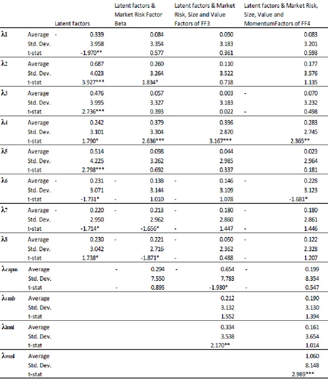
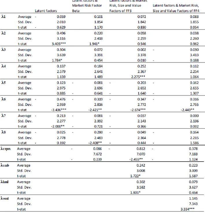
Table 7. Cross Sectional Regression of Individual Portfolios

One star (*), two stars (**) and three stars (***) show that the factors are significant at 10%, 5% and 1%, respectively.

A summary of the statistical values of the lambdas that correspond to the latent factors of the individual portfolio models can be found in Table 7. The figures in the table exhibit that when the model is constructed by just eight latent factors; there is no insignificant lambda at the

(50)

40

10% critical level. When one more factor, market risk, value or size factor, is added to the model, the significance of the independent variables are reduced according to the t statistics. The findings in Table 7 provide an important result for the study of the financial sector. Consumption series, money and credit sector related variables and stock market variables have significant effects on the model constructed with individual portfolios, in particular when the CAPM coefficient is added to the model.

Additionally, the adverse effects of the additional factors on the significance of the latent macroeconomic factors in explaining the total variation in the individual portfolio model, can also be seen clearly.

(51)

41

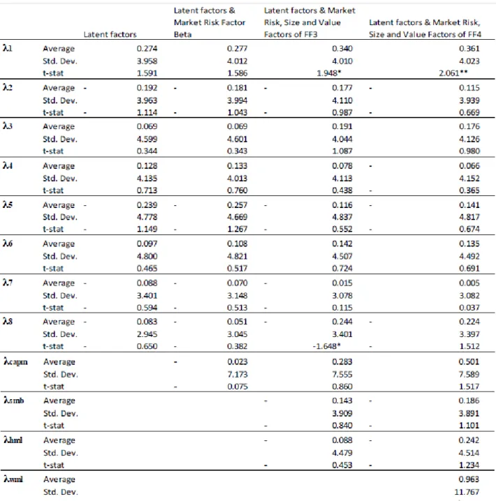
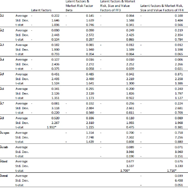
Table 8. Cross Sectional Regression of Industry Portfolios

Table 8 shows the result of the cross sectional regression which is conducted with the Industry Portfolios of Fama French model. Unlike the regression with individual portfolios, in this model (industrial portfolio model), the latent factors do not have significant effects on the stock returns. There are only two significant factors, 1 and 8, for the returns if additional factors, market risk, value and size, are included in the model besides the latent factors. The

(52)

42

situation becomes worse when the momentum factor is added to the model so that only factor 1 has a significant effect on stock returns.

Table 9. Cross Sectional Regression of Individual Portfolios in Expansion Periods

(53)

43

Table 10. Cross Sectional Regression of Individual Portfolios in Recession Periods

In the next two tables, 9 and 10, the boom and recession periods in the cross sectional regressions are specified in the model and the results are interpreted for the individual portfolios. In contraction periods, the latent macroeconomic factors have no significant effect in explaining the variation in stock returns. There is only one significant factor, Factor 8,

(54)

44

when the model is constructed with only latent factors. However, there are more significant latent factors for the portfolio return in the boom periods.

Table 11. Comparison of Cross Sectional Regressions

Table 11 shows the average and the adjusted average R squared. According to the table, 25% to 54% of the cross sectional variation can be explained by the factors for each model. The R squared is getting to increase by adding each additional Fama French three model or momentum factors. The adjusted R squared values are almost same with the R squared; the only difference is that the adjusted one has smaller increments since the degree of freedom is taken into account in calculating the adjusted R squared. Besides the interpretation of the R squared, another indication of the figures in Table 11 is that the explained parts of the stock returns are higher in the contraction periods compared to the boom periods.

(55)

45

6. CONCLUSION

As global financial crises became the major issue on the agenda over last few decades, there are various studies about the relationship between the macroeconomic variables and the stock returns. Martinez & Rubio (1989) and Poon & Taylor (1991) analyzed the relationship between the macroeconomic variables and the stock returns in the UK and Spanish stocks market, respectively. They could not find any significant effect. This thesis and various others in the literature found important relationships between the macroeconomic variables and the stock returns. Gunsel & Cukur (2007) and Rjoub, Tursoy and Gunsel (2009), for instance, have found close relationships between many macroeconomic variables in London Stock Exchange and Istanbul Stock Exchange, respectively. Moreover, using econometric models (discussed in the literature), many studies on different countries with different found that some macroeconomic factors have significant effects on the stock returns. In this study, it is found that some macroeconomic variables have significant influence on stock returns which in the U.S. stock market.

This study disembarks from related other studies in the literature such that the effects of macroeconomic factors on the stock returns are analyzed by APT but these factors were extracted by the principal component analysis, which is the most appropriate method (Stock and Watson, 2002 and Bai and Ng, 2002). The analysis was repeated for four different models created by adding the market risk factor, size and value factors and momentum factor to the basic model which includes only the latent factors. These models are used to examine the relationships between the macroeconomic factors and the stock returns using different data sets, namely, 100 individual portfolios, 49 industry portfolios and recessions and expansion periods for the individual portfolio data set.

(56)

46

Post and Levy (2005) state that size and value factors have a significant effect in explaining the stock returns and the momentum factor is stronger than the size and value factors to determine the expected stock returns. Also, Chan, Chen and Hsieh (1995) concluded that the size factor matters in explaining the stock returns. However, in this thesis, although the size, value and momentum factors are found to have some effect to increase the R squared of the models, this increase is less than expectations. Hence, these additional factors have positive effects regarding the explanatory power of the model but the significance level of the macroeconomic factors has decreased when these additional factors are inserted into the model.

Previous studies generally found that different macroeconomic variables have significant effects on the stock returns. The common variables are industrial production, the inflation rates (expected and unexpected), term structure of the risk premium, the interest rate and oil prices (Cauchie et al. 2003; Hamao, 1998; Chen et al, 1986). In our study, the factors in group 2 (labor market) and group 8 (stock market) are common significant factors for the stock returns in almost all models. Ludvingson and Ng (2009) found the same result; these two factors are the most important of all factors.

The main finding of this thesis is that the latent factors which are extracted from the macroeconomic data by the principal component analysis have significant relationship with the stock returns in the U.S. With this result, this study joins previous studies which found significant effects of macroeconomic factors on stock returns.

(57)

47

If a model is constructed with only the latent factors which are derived from the macroeconomic series, these factors can be priced as risk factors. In this study, three more additional models are constructed by adding CAPM coefficient or market risk factor, value and size factors and also the momentum factor in order to find the best model that explains higher variation in the stock returns. Some of these potential factors are still important but some turn into minor risk factors. This demonstrates that these additional factors have the capacity to explain the cross section of stock returns as much as the extracted latent factors. The results differ tremendously when various portfolios are used. This thesis includes two different portfolios to create the structure of the data, individual portfolios and industrial portfolios. When certain types of portfolios like industry portfolios are evaluated, the latent factors are no longer assessed as risk factors. Finally, it is found that latent factors do not function in a similar way in explaining the cross sectional variation for boom and recession periods. As to recession periods, almost all of the latent factors lack an explanatory power. This might be due to the short downturn periods and unusual rise and fall in the returns. In other respects, for the growth periods, a part of latent factors remain important.

This paper can be improved in different ways for further research. The analysis can be repeated by adding some other assets, bonds, etc. to analyze the relationship between the macroeconomic variables and other potential dependent variables, not just stock returns. Moreover, this analysis can be done for other countries’ stock markets or other markets to examine the effects of the latent factors. The use of techniques other than the principal component analysis to find the factors also remains as a possible opportunity for further research.

(58)

48

References

 Adam, A.M. and G. Tweneboah, (2008), “Macroeconomic factors and stock market movement: Evidence from Ghana”, Munich Personal RePEc Archive, No. 14079

 Akay, H. K., & Nargeleçekenler, M. (2009), “Para Politikası Şokları Hisse Senedi Fiyatını Etkiler mi? Türkiye Örneği”, Marmara Üniversitesi İİBF Dergisi, 27(2): 129-152

 Aktas, E. (2011), “Systematic factors, information release and market volatility”, Applied Financial Economics, 21(6): 415-420

 Ali, I., Rehman, K. U. , Yilmaz, A. K. , Khan, M. A. & Afzal, H. (2010), “Causal relationship between macro-economic indicators and stock exchange prices in Pakistan”, African Journal of Business Management , 4(3): 312-319

 Alshogearthi, M. (2011), “Macroeconomic determinant of the stock market movement: empirical evidence from the Saudi stock market”, Kansas State University, 89-98

 Altay, E. (2003), “The Effect of Macroeconomic Factors on Asset Returns: A Comparative Analysis of the German and the Turkish Stock Markets in an APT Framework”, Journal of Finance, 43 (2):327-338

 Aydemir, O. and E. Demirhan, (2009), “The relation between stock prices and exchange rates: Evidence from Turkey”, International Research Journal of Finance and Economics, 23: 207-215

 Bai, J., and Ng, S. (2000), “Determining the Number of Factors in the Approximate Factor Models”, Econometrica, 70: 191-221

 Bodurtha, J. N., Cho, D.C.Y. and Senbet, L. (1989), “Economic Forces in the Stock Market”, Global Finance Journal, 1: 21-46.

 Cauchie, S., Hoesli, M. and Isakov, D. (2003) “The determinants of stock returns in a small open economy: Swiss stock market”, National Centre of Competence in Research Financial Valuation and Risk Management, 80:167-185

 Chamberlain, G., and M. Rothschild (1983), “Arbitrage Factor Structure, and Mean-Variance Analysis of Large Asset Markets,” Econometrica, 51:1281-1304

 Chan, K. C., Chen, N. F. and Hsieh, D. A. (1985), “An Explanatory Investigation of the Firm Size Effect”, Journal of Financial Economics, 14:451-471

 Chen, N. F., Roll, R., Ross, S. (1986), “Economic Forces and the Stock market”, Journal of Business, 59: 383-403