IS S N 1 3 0 3 –5 9 9 1
ESTIMATING THE EARTHQUAKE SOURCE PARAMETERS: SIMULATED ANNEALING VERSUS NELDER-MEAD SIMPLEX
ALGORITHM
ÖZLEM TÜRK¸SEN AND AY¸SEN APAYDIN
Abstract. The parameter estimation is an important process in many earth science problems in order to de…ne the features of ground movement. It is clear that the model nonlinearity makes the estimation of parameters more di¢ cult and more challenging. In this case, metaheuristic algorithms and derivative free optimization methods are more proper than classical optimization meth-ods. In this study, Simulated Annealing (SA), a well known metaheuristic algorithm, and Nelder-Mead simplex algorithm, a derivative free optimization method, are used to estimate the earthquake source parameters. The algo-rithms are applied on a synthetically generated data set. The estimated para-meter results show that the SA is better than Nelder-Mead simplex method.
1. Introduction
An earthquake is de…ned by source parameters. Modeling of the source parame-ters requires wide knowledge of elastic half space theory due to the elastic structure of the crust. Many past attempts to infer source geometry from deformation …elds have used elasticity theory to …nd geologically plausible models that …t the major features of the observed deformation …eld. The fault plane is used to determine surface displacements on de…nite coordinates. The correct estimation of source pa-rameters gives good predictions for the next earthquake occurance. In this case, the estimation of the fault plane parameters becomes important as modeling. Many new methodologies have been developed in the …eld of estimating the source para-meters [9, 11, 20, 22]. Derivative based searching algorithms; e.g., a Quasi-Newton method [6], derivative free optimization algorithms; e.g., Nelder-Mead simplex al-gorithm [5, 15], heuristic optimization methods; e.g., SA alal-gorithm [2, 3, 7, 21] and genetic algorithms [8, 18], Monte-Carlo methods [26] are used for the estimation of crust model parameters.
Received by the editors May 23, 2013; Accepted: Nov. 21, 2013. 2000 Mathematics Subject Classi…cation. 65C60, 49N45, 90C30, 65K10.
Key words and phrases. Simulated Annealing, Nelder-Mead simplex algorithm, parameter es-timation, fault plane parameters.
c 2 0 1 3 A n ka ra U n ive rsity
In this study, SA algorithm is used to estimate the earthquake source parame-ters using analitical solution for deformation. The SA algorithm is a random search method based on the analogy between cooling and the freezing of the metals and some liquid materials at crystal structure with minimum energy and researching the minimum of a general system. The SA is based upon that of [24], which was originally proposed as a means of …nding the equilibrium con…gurations of a col-lection of atoms at a given temperature. Kirkpatrick [19] was …rst proposed the algorithm basis of an optimization technique for combinatorial problems. The SA permits the e¢ cient period for the dispersion of the molecules again by decreasing the temperature gradually. Thus, the method can be considered as a minimization algorithm based on natural events and nature. Also the SA is a stochastic computa-tional method with quick approximations to global solutions for hard optimization problems in di¤erent …elds [10, 13, 28, 16, 17, 27, 30, 31]. The SA algorithm has advantages in dealing with the strong nonlinearities and discontinuities in the hilly structure of cost function. This paper describes the SA algorithm and explores its ability to optimize NP-hard functions in geosciences through an e¢ cient explo-ration of the parameter space. And also the paper gives a comparison for parameter estimation with a derivative free optimization method, called Nelder-Mead simplex method [25]. The synthetically generated data set is used for the application. All the calculations are done by using Matlab.
The rest of the paper is organized as follows: In Section 2 fault plane geometry is showed and inverse problem formulation is presented. In the next section the SA algorithm is brie‡y reviewed and the implementation of SA algorithm to fault plane parameter estimation procedure is given. This is followed by simulation results that illustrates the both proposed approaches via the Monte Carlo simulation. In the last part, numerical results of the estimations are compared and the performance of the optimization algorithms is analyzed.
2. Fault Plane Model and Inverse Problem Formulation
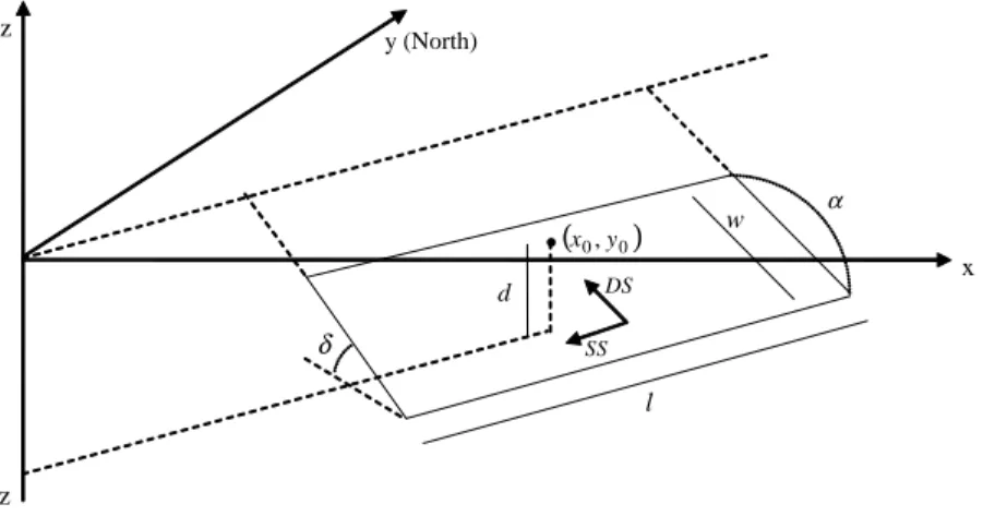
2.1. The fault plane geometry. The fault plane parameters play an important role for de…ning the characteristics of surface displacements. It is a hard work to estimate earthquake source parameters and it requires a well de…ned model. The most commonly used crustal model is the homogeneous, isotropic, linear, and elastic half-space. In spite of its limitations, the elastic half space model is widely used because of the simplicity of the expressions [7]. Figure 1 illustrates the fault plane geometry in three dimensions.
x y (North) d α δ
.
(x0, y0) z SS DS w -z lFigure 1. The fault geometry and the relocation on the fault
The parameters de…ned on the fault plane in Figure 1 are l : the lenght of the fault plane (km),
w : the wideness of the fault plane (km), d : the depth of the fault plane (km),
: dip angle (radian), : strike (radian),
(xf; yf ) : the coordinates of the fault starting point where xf (km) is east ofset and yf (km) is north ofset,
SS : the component of the slip vector (S) in the direction of the fault (Strike-Slip) (m),
DS : the component of the slip vector (S) as vertical to the fault direction (Dip-Slip) (m),
(x0; y0) : the location of the fault center de…ned on the surface.
In this study, a plate model, which is expressed by Aktu¼g [4], is considered because of its simplicity and speed in computing. In the model surface relocations, caused by the slip vector, is de…ned as analitical equations for quadrangular area. The slip is consist of two components such as “lateral range”in the direction of the fault plane and the “vertical range” as vertical to lateral range. The both range functions are given below:
Lateral range : ux = u1 2 q R (R + )+ tan 1 qR+ I1sin uy = u1 2 y0q R (R + )+ q cos R + + I2sin uz = u1 2 d0q R (R + )+ q sin R + + I4sin Vertical range : ux = u2 2 q R+ I1sin cos uy = u2 2 y0q R (R + )+ cos tan 1 x R + I1sin cos uz = u2 2 y0q R (R + )+ sin tan 1 qR I5sin cos
where the I1; I2; I3; I4; I5 are analitical equations and contain source parameters. These equations are consist of nonlinear combinations of the fault plane parameters. The reader is referred to the works by [4] for a detailed description of parameters. The equation systems, given above with lateral and vertical ranges, show the func-tional relations between the fault geometry and surface displacements. Because of the nonlinearity of these complex analitical functions, classical parameter estima-tion methods may fail. In this case, estimaestima-tion of fault plane parameters by the SA algorithm makes certain facilities to get global solutions; e.g. providing su¢ -cient convergence, escaping local traps, easy implementation to real world NP hard optimization problems.
2.2. Inverse problem formulation. One of the main aim of geophysical inversion is to identify the all models which give an acceptable loss between predicted and observed data. In terms of the loss function, a measure of the di¤erence between observed and synthetic data that varies as a function of solution parameters [23]. In this study, the inversion problem, which describes the geometry and the slip of the fault plane, is formed with analitical lateral and vertical range equations.
Let p be the nine dimensional vector whose elements pj are the geometrical source parameters wanted to be estimated denoted by p [l w d xf yf SS DS]. Let g g(p) g1 g2 gN be the N -dimensional vector whose ith ele-ment gi, i = 1; 2; :::; N is the surface relocation vector with three dimensions (x; y; z) at the ith observation point. Therefore, the observed surface displacements u can be written as a function g of the fault model parameters p
where e is a vector of observational errors. The surface relocation vector u consists of two components as in the lateral direction, ul = ul
x; uly; ulz and in the vertical direction, uv= uv
x; uvy; uvz . Thus, the equation 2.1 can be written as
uij=gij(p) + eij , i = 1; 2; :::; 50 , j = x; y; z. (2.2) The surface displacements are related nonlinearly to the fault plane parameters as seen from the lateral and vertical equations. Hence, the estimation of the fault plane parameters becomes to a nonlinear optimization problem. Estimating p from gis formulated as the minimization of the function f given
f (u; g) = ku g(p)k2 (2.3)
where k k is the Euclidean norm. The optimal parameter values p minimize the L2 norm of the loss function given by 2.3, which is considered as an objective function [29]. Therefore, the nonlinear unconstrained optimization problem can be written as
min f (u; g)
p2 S (2.4)
where S is the domain of parameters.
The analytical solution of the problem seems to be unavailable because of the nonlinearity of fault plane model. The size of parameter space, the existence of local minima, the continuity of objective function and the sensitivity of objective function to each of the model parameters must be considered. In order to solve the inverse problem commonly used techniques such as simple Monte Carlo methods become ine¢ cient or impractical in very large solution spaces. More recently a number of guided search techniques from the …eld of arti…cial intelligence and heuristic methods have been developed. In this study, SA is used to estimate the overall earthquake geometry using the optimization problem given with lateral and vertical equations.
3. Application of the SA algorithm to the estimation problem The SA algorithm derives its name from an analogy to the cooling of metals. As a metal cools, the atoms ‡uctuate between relatively higher and lower energy levels. If the temperature is dropped slowly enough, the atoms will all reach their ground state. This cooling process is called as “annealing”. However, if the temperature is dropped too quickly, the system will get trapped in a less than optimum con…gura-tion. So the temperature is considered as the control parameter in the method. If the energy function of this physical system is instead replaced by an objective func-tion, then the progression of this function towards the global minimum is analogous to the physical progression towards the ground state.
Convenience of application to real world problems and obtainment of good solu-tions makes the SA algorithm be one of the most powerful and popular heuristics
to solve many optimization problems. Some factors need to be considered when designing the SA algorithm. The following elements must be provided for imple-menting the SA to a problem:
(i) are presentation of possible solutions, (ii) a generator of random changes in solutions,
(iii) a means of evaluating the probability functions, and
(iv) an annealing schedule, an initial temperature and rules for lowering it as the search progresses[1].
The optimization problem given in equation 2.4 will be minimized to estimate the nine fault plane parameters with the SA algorithm. The algorithm has two cycles, inner and outer. A neighboring parameter set of the current parameter set is generated, in the inner cycle of the algorithm. If the new state is better than the current state then the generated solution replaces the current solution, otherwise the solution is accepted with a criterion probability. The value of the temperature, control parameter, decreases in each iteration of the outer cycle of the algorithm. In this regard, the steps of this algorithm are brie‡y looked into:
Step 1: T0 is chosen as the initial temperature, p0 is chosen arbitrarily as an initial parameter set on the de…nition space, n is the dimension of fault parameter set, Tminis chosen as the …nal temperature (stopping criteria of outer cycle), L is chosen as the number of neighborhood solutions generated at a certain temperature T to get equilibrium (stopping criteria of inner cycle), a and b are chosen lower and upper bound sets for parameters respectively. Firstly, the initial temperature is considered as the system temperature, Tk= T0 for k = 0 and optimal parameter value p is set to p0, p = p0.
Step 2: Under kth temperature, if the inner loop condition is met, go to Step 3 ; otherwise the new parameter set is produced at a given temperature as
pj+1= pj+ y (b a) , y2 rand ( 1; 1) (3.1)
where, p is constrained by p 2 [a; b] . Later on, the new function value f (pj+1) = fj+1and f = fj+1 fjare computed. If f < 0, the new state is accepted. Otherwise, the Metropolis criterion is followed to accept pj+1with a probability of min 1; e Tkf and Step 2 continues.
Step 3: The temperature is reduced according to a speci…ed cooling schedule, Tk = T0ck , 0 < c < 1, where c is analogous to the Boltzmann’s constant that can be used to tune the algorithm. If outer loop break condition is met computation stops and optimal parameter set is reached. Otherwise, Step 2 is repeated.
The de…nition of the starting temperature, the cooling schedule of the tempera-ture, the iteration number at each temperature and the de…nition of the stopping criteria have great roles in the e¢ ciency of the algorithm [12]. Various SA algo-rithms are based on the same principle explained above, e.g., Boltzmann annealing [19], fast simulated annealing [28], very fast simulated annealing [16], and adap-tive simulated annealing [17]. These algorithms vary in probability distribution,
annealing schedule, and the generation methods of random change. In this study, geometric cooling schedule is chosen and applied to earthquake source parameter estimation scheme.
4. Numerical Example
In this section, a numerical example is used to investigate the performance of the SA algorithm. An operation region is de…ned for performing the simulated data. The surface relocations, taken as outputs of the estimation scheme, are generated on the experimental region for de…ned coordinates using Matlab code. It is tried to get the optimal values of fault plane parameters. In the conclusion part of the simulation study, SA and Nelder-Mead simplex algorithm are compared in terms of their convergency to optimal value of nine source parameters.
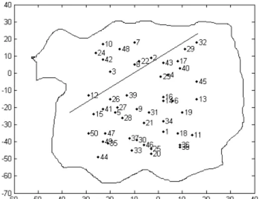
4.1. Data. An operation region, a quadrangular area, is de…ned for performing simulated data and considered as a de…nite place of earth surface where earthquake has been occured. The simulated earthquake area is formed in ( 30; 20) ( 50; 20) coordinates with 50 geodetic points which are signed on the graph given in Figure 2.
Figure 2. De…ned 50 coordinates around the fault direction
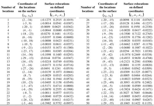
As can be seen from the Figure 2 that the fault direct, passed along the origin with a straight line, is formed and 50 random generated coordinate values (x; y) are …xed around the fault direction. The surface relocations, denoted as [x; y; z], are generated by using Matlab code taken from the geodynamics laboratory page (http:// www.gpsg.mit.edu) of the Massachusetts Technology Institute for each coordinate. The …xed 50 coordinates and the surface relocations are given in Table 1. The fault plane parameters, used for synthetic data set and the lower and the upper bounds of the parameters are presented in Table 2.
Table 1. The coordinates of locations and relocations
Coordinates of Surface relocations Coordinates of Surface relocations Number of the locations on defined Number of the locations on defined
locations on the surface coordinates locations on the surface coordinates
(x0, y0)
(
ux,uy,uz)
(x0, y0)(
ux,uy,uz)
1 (2 , -34) (-0.1275 0.2515 -0.1019) 26 (-20 , -15) (0.0098 0.1118 -0.0765) 2 (-3 , 9) (-0.0014 0.0541 -0.0307) 27 (-17 , -20) (0.0128 0.1496 -0.1237) 3 (-20 , 1) (0.0009 0.0625 -0.0362) 28 (-15 , -26) (0.0101 0.1950 -0.2330) 4 (4 , -1) (-0.0044 0.0680 -0.0393) 29 (11 , 14) (-0.0020 0.0417 -0.0222) 5 (-18 , -23) (0.0270 0.1681 -0.1532) 30 (-9 , -39) (-0.3500 0.7122 -0.2765) 6 (6 , -16) (-0.0197 0.1046 -0.0600) 31 (-4 , -23) (-0.0339 0.1756 -0.1282) 7 (-10 , 18) (-0.0008 0.0423 -0.0231) 32 (16 , 18) (-0.0020 0.0355 -0.0183) 8 (-10 , 5) (-0.0010 0.0611 -0.0357) 33 (-11 , -45) (-0.6662 1.0287 -0.1170) 9 (-9 , -21) (-0.0153 0.1673 -0.1380) 34 (2 , -28) (-0.0680 0.1887 -0.1022) 10 (-23 , 17) (-0.0001 0.0385 -0.0204) 35 (-21 , -41) (0.0294 -0.7021 1.0330) 11 (14 , -36) (-0.1098 0.1485 -0.0293) 36 (9 , -42) (-0.1974 0.2469 -0.0338) 12 (-29 , -13) (0.0144 0.0736 -0.0367) 37 (-12 , -38) (-0.4933 0.9630 -0.4768) 13 (16 , -15) (-0.0218 0.0749 -0.0350) 38 (9 , -43) (-0.2121 0.2581 -0.0308) 14 (2 , -16) (-0.0173 0.1154 -0.0716) 39 (-13 , -13) (0.0001 0.1155 -0.0820) 15 (-27 , -24) (0.0491 0.1241 -0.0519) 40 (9 , 3) (-0.0041 0.0562 -0.0309) 16 (2 , -14) (-0.0139 0.1073 -0.0664) 41 (-23 , -21) (0.0309 0.1325 -0.0877) 17 (8 , 7) (-0.0029 0.0515 -0.0283) 42 (-23 , 8) (0.0005 0.0484 -0.0264) 18 (8 , -35) (-0.1184 0.1944 -0.0574) 43 (2 , 6) (-0.0023 0.0569 -0.0323) 19 (10 , -23) (-0.0405 0.1158 -0.0549) 44 (-25 , -49) (0.3093 -0.1076 0.2482) 20 (-3 , -47) (-0.5171 0.6714 -0.0800) 45 (16 , -5) (-0.0100 0.0589 -0.0300) 21 (-6 , -29) (-0.0870 0.2555 -0.1988) 46 (-6 , -42) (-0.3824 0.6424 -0.1471) 22 (-8 , 7) (-0.0011 0.0577 -0.0333) 47 (-22 , -35) (0.3027 0.7685 -0.0648) 23 (1 , -2) (-0.0040 0.0729 -0.0432) 48 (-16 , 14) (-0.0005 0.0453 -0.0249) 24 (-26 , 12) (0.0005 0.0412 -0.0217) 49 (-23 , -40) (-0.1164 0.0907 0.6267) 25 (-3 , -44) (-0.3982 0.5752 -0.0957) 50 (-29 , -35) (0.1065 0.1422 0.1135)Table2. The true values and the de…nition intervals of the fault plane parameters Parameters Parameter Values Bounds of Parameters Lenght (km) 60 20 - 100 Width (km) 12 5 - 15 Depth (km) 1 0 - 5 Dip (radian) 1.2217 0.8727 - 2.0944 Strike (radian) 5.4978 4.7124 - 6.2832 East offset (km) -20 -50 - 0 North offset (km) -40 -50 - 0 Strike Slip (m) 2 -5 - 5 Dip Slip (m) 0.2 -5 - 5
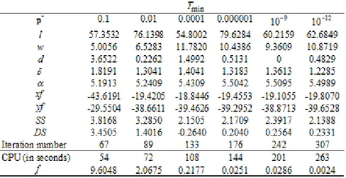
4.2. Results of the SA algorithm. The objective function is analyzed in the parameter space during the parameter optimization procedure with SA algorithm. In the absence of any prior information about where the good feasible solutions might lie, it’s reasonable to set each parameters midway between its lower bound and upper bound in order to start the search in the middle of the feasible region. For a sample run, initial parameter set is taken
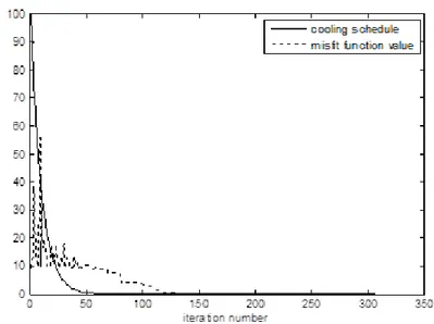
p0 = [60 10 2.5 1.48355 4.5978 -25 -25 0 0]. The initial temperature and Boltz-mann’s constant are considered T0and c = 0:9, respectively. The inner loop break condition is taken n 10, where n is the dimension of parameter set. Table 3 shows the results of SA algorithm for di¤erent stopping criteria (Tmin). For each Tmin, the iteration number and computation time (CPU) are shown together with the objective function value (f ) and estimated values of source parameters (p ). It can be seen from the Table 3 that when the Tmin is decreased the loss function value gets smaller and the calculation period gets longer. The objective function takes the smallest value when the stopping criteria is choosen 10 12. The change on temperature and the minimization of loss function value during the search process of SA are given in Figure 3. It can be seen from Figure 4 that while the tempera-ture drops constantly from the beginning of the search, the objective function value given in equation 2.3 reaches the global minimum value.
Figure3. Cooling schedule and loss (mis…t) function value of SA for Tmin= 10 12
Figure 4 shows the estimation results of source parameters during the search processes. The broken line illustrates the true values of the parameters. It’s quite clear that the estimated values of the source parameters are very close to the true values, given in Table 2, while the algorithm gets the global minimum.
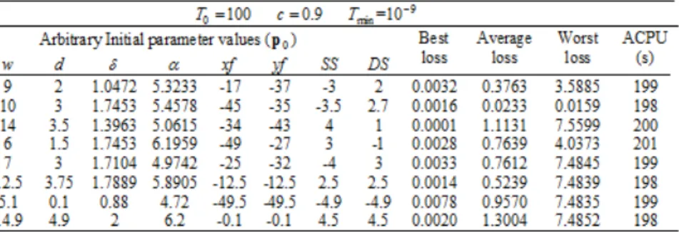
A single run of global converging algorithms is not su¢ cient to …nd the global so-lutions. The model parameters obtained by several runs may di¤er from each other because of the stochastic structure of the algorithm. Since the SA is a probabilistic search algorithm, di¤erent runs may result in dissimilar con…gurations. Therefore, several seperate runs are performed to ensure that the true global minimum has been located. The average results of 100 Monte Carlo simulations for the di¤erent initial values of fault plane parameters and average computation times (ACPU) are reported in Table 4. The initial temperature, Boltzmann’s constant and stopping criteria are choosen 100, 0.9, and 10 8 respectively for all test runs. It has been observed from the simulation results that the average loss function value converges the global minimum for the arbitrary initials. It can be easily said that SA largely independent of the initial values and it can escape local minima through selective uphill moves.
Table 4. The loss function values for the di¤erent initials
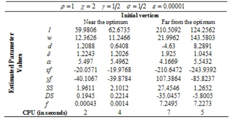
4.3. Results of the Nelder-Mead simplex method. The tests have been made on starting points chosen near the optimum and quite far from the optimum gen-erated inside the parameter interval. Four scalar parameters must be speci…ed to de…ne a complete Nelder-Mead simplex method; coe¢ cients of re‡ection , expan-sion , contraction , and shrinkage . These parameters are chosen to satisfy > 0, > 1, 0 < < 1, and 0 < < 1. In this study, Nelder-Mead simplex algorithm, composed by [14], is applied to the source parameter estimation scheme. The coe¢ cients of re‡ection, expansion, contraction and shrinkage are choosen = 1, = 2, = 12, and = 12, respectively. The stopping criteria is considered " = 0:00001. The results of Monte Carlo simulations are given in Table 5. It can be seen from the results that the Nelder-Mead simplex method requires stringent initial estimates for the model parameters. The method is only advantageous when a good initial estimate is provided. If the initial vertices are generated far from
optimum, the loss function (f ) can not reach the global minimum and CPU time gets large.
Table 5. The simulation results of Nelder-Mead simplex algorithm
5. Conclusions
Estimation of fault plane parameters using classical optimization methods, e.g., derivative-nonderivative based optimization methods, Monte-Carlo methods, Least Squares methods, etc. is often di¢ cult because of the nonlinearity of the problem. These methods need some assumptions to implement on problems and also may fail to get global solutions of optimization problems. In this paper, SA algorithm is presented and compared with a derivative-free optimization method, Nelder-Mead simplex method, for estimating the source parameters. The SA algorithm has many advantages over other optimization methods. The method has advantages in dealing with strong nonlinearities and discontiniuties. The SA algorithm sometimes goes uphill as well as downhill unlike other direct optimization methods. This is an ability to avoid becoming trapped at local minima.
During the Monte Carlo simulation study, it’s realized that assessing the per-formance of the Nelder-Mead simplex method is generally problematic due to the nonconverge of optimal parameter values even if it is more e¢ cient than other direct search optimization methods. The simplex method requires strict initial conditions, whereas the SA algorithm is able to explore the parameter space and focus on the most promising area without prior knowledge of its location. The simulation results show that the SA algorithm is an e¢ cient derivative-free optimization algorithm with respect to Nelder-Mead simplex method. However, the SA has some draw-backs. The most remarkable disadvantages of the SA algorithm are (i) spending much computing time to …nd the optimum solution and (ii) determining the proper cooling schedule. In order to obtain better results, the various tunable parameters used (e.g. initial temperature, …nal temperature, cooling rate etc.) needed to be chosen carefully depending on the problem variety.
Due to its versatility and independence on prior knowledge of the parameter values, the SA algorithm is particularly applicable to estimate the parameters of fault plane model that are not solvable using analytical methods. It can be said that the SA algorithm is a promising tool for estimation of parameters in geosciences. However, the utility of this procedure to estimate fault plane parameters from real data has yet to be proven. In the later studies, it’s possible to improve the algorithm by using di¤erent cooling schedules. Using a hybrid optimization strategy based on SA and gradient based or direct optimization algoritm can provide more e¢ cient and accurate estimation of parameters. On the other hand as there are other well-established heuristics, such as genetic algorithms, Bee and Ant Colony, etc., a discussion of how good the estimation can be achieved by using them, may lead to a better estimation procedure.
References
[1] Abbasi, B., Jahromi, A.H.E., Arkat, J. and Hosseinkouchack, M., Estimating the parame-ters of Weibull distribution using simulated annealing algorithm, Applied Mathematics and Computation, 183, 85-93, (2006)
[2] Abdel-Fattah, A.K., An approach to investigate earthquake source processes, Acta Geophys-ica PolonGeophys-ica, 51(3), 257-269, (2003)
[3] Abdel-Fattah, A.K. and Badaway, A., Source Characteristics and Tectonic Implications of Moderate Earthquake, Northeastern Cairo Prefecture. Acta Geophysica Polonica, 52(1), 29-43, (2004)
[4] Aktu¼g, B., A Dynamic Approach to Elastic Half Space Models and Earthquake Coordinate Relocations, Map Journal, 129, 1-16, (2003)
[5] Ateya, I.L. and Takemoto, S., Gravity inversion modelling across a 2-D dike-like structure-A Case Study, Earth Planet Space, 54, 791-796, (2002)
[6] Arnadottir, T. and Segall, P., The 1989 Loma Prieta earthquake imaged from inversion of geodetic data, Journal of Geophysical Research, 99(B11), 21835-21855, (1994)
[7] Carvelli, P., Murray, M.H., Segall, P.,Aoki, Y. and Kato, T., Estimating source parameters from deformation data, with an application to the March 1997 earthquake swarm of Izu Peninsula, Japan, Journal of Geophysical Research, 106(B6),11217-11238, (1999)
[8] Chang, S.J., Baag, C.E. and Langston, C.A., Joint analysis of teleseismicreceiver functions and surface wave dispersion using the genetic algorithm, Bulletin of the Seismological Society of America, 94, 691-704, (2004)
[9] Charlety, J., Vallee, M. and Delouis, B., Fast Source Parameter Estimation from Green Func-tion DeconvoluFunc-tion: ApplicaFunc-tion to Shallow Earthquakes. Geophysical Research Abstracts, 10, EGU2008-A-06557, (2008)
[10] Corana, A., Marchesi, M., Martini, C. and Ridella, S., Minimizing multimodal functions of continuous variables with the “simulated annealing” algorithm. ACM Transactions on Mathematical Software, 13, 262- 280, (1987)
[11] Del Frate, F., Rossi, F., Schiavon, G. and Stramondo, S., Seismic Source Parameters from InSAR Data Trough Neural Networks, IEEE, 2981-2984, (2004)
[12] Eglese, R.W., Simulated Annealing: A tool for Operational Research, European Journal of Operational Research, 46, 271-281, (1990)
[13] Go¤e, W.L., Ferrier, G.D. and Rogers, J., Global optimization of statistical functions with simulated annealing, Journal of Econometrics, 60, 65-99, (1994)
[14] Hedar, A.R., Studies on Metaheuristics for Continuous Global Optimization Problems, 2004, Ph.D. Thesis, Kyoto University, Japan, 148pp.
[15] Ichinose, G.A., Smith, K.D. and Anderson, J.G., Source Parameters of the 15 November 1995 Border Town, Nevada, Eathquake Sequence, Bulletin Seismological Society of America, 87(3), 652-667, (1997)
[16] Ingber, L., Very Fast Simulated Re-Annealing, Mathematical Computer Modelling, 12(8), 967-973, (1989)
[17] Ingber, L., Simulated Annealing: Practice versus Theory, Mathematical Computer Modelling, 18(11), 29-57, (1993)
[18] Kim W., Hahm I.K., Ahn S.J. and Lim D.H., Determining hypocentral parameters for local earthquakes in 1-D using a genetic algorithm, Geophysical Journal International, 166, 590-600, (2006)
[19] Kirkpatrick, S., Gelatt, C.D. and Vecchi, M.P., Optimization by Simulated Annealing, Sci-ence, 220(4598), 671-680, (1983)
[20] Kumar, B.A., Ramana, D.V., Kumar, Ch.P., Rani, V.S., Shekar, M., Srinagesh, D. and Chadha, R.K., Estimation of source parameters for 14March2005 earthquake of Koyna-Warna region, Current Science, 91(4), 526-530, (2006)
[21] Li, X., Koike, T. and Pathmathevan, M., A very fast re-annealing (VFSA) approach for land data assimilation, Computers and Geosciences, 30, 239-248, (2004)
[22] Lin, T.W., Hwang, R.D., Ma, K.F. and Tsai, Y.B., Simultaneous Determination of Earth-quake Source Parameters Using Far-Field P Waves: Focal Mechanism, Seismic Moment, Rup-ture Length and RupRup-ture Velocity, Terrestrial Atmospheric And Oceanic Sciences, 17(3), 463-487, (2006)
[23] Lomax, A. and Snieder, R., Identifying sets of acceptable solutions to non-linear, geophysical inverse problems which have complicated mis…t functions, Nonlinear Processes in Geophysics, 2, 222-227, (1995)
[24] Metropolis, N., Rosenbluth, A.W., Rosenbluth, M.N. and Teller, A.H., Equation of State Calculations by Fast Computing Machines, The Journal of Chemical Physics, 21(6), 1087-1092, (1953)
[25] Nelder, J.A. and Mead, R., A simplex method for function minimization, Computer Journal, 7, 308-313, (1965)
[26] Sambridge, M. and Mosegaard, K., Monte-Carlo Methods in Geophysical Inverse Problems, Reviews of Geophysical, 40(3), 1-29, (2002)
[27] Sharma, S.P. and Kaikkonen, P., Global Optimization of Time Domain Electromagnetic Data Using Very Fast Simulated Annealing, Pure and Applied Geophysics, 155, 149-168, (1999) [28] Szu, H. and Hartley, R., Fast Simulated Annealing, Physics Letters A, 122(3,4), 157-162,
(1987)
[29] Türk¸sen, Ö. The Adaptive Simulated Annealing Method in Estimation of Earthquake Search Parameters Through Surface Measuraments, 2005, Master Thesis, 72pp.
[30] Vasan, A. and Raju, K.S., Comparative analysis of Simulated Annealing, Simulated Quench-ing and Genetic Algorithms for optimal reservoir operation, Applied Soft ComputQuench-ing, 36, 274-281, (2009)
[31] Xu, T., Wei, H. and Wang, Z.D., Study on continuous network design problem using simulated annealing and genetic algorithm, Expert Systems with Applications, 36, 2735-2741, (2009) Current address : Ankara University Faculty of Science, Department of Statistics, 06100,
Tan-do¼gan, Ankara,TURKEY
E-mail address : [email protected], [email protected]