A FEASIBILITY ANALYSIS TO FIND THE OPTIMAL LOCATION FOR A SOLAR POWER BY USING MCDM METHODS; A CASE STUDY IN TURKEY

(1)

T.C.

ISTANBUL AYDIN UNIVERSITY INSTITUTE OF GRADUATE STUDIES

A FEASIBILITY ANALYSIS TO FIND THE OPTIMAL LOCATION FOR A SOLAR POWER BY USING MCDM METHODS; A CASE STUDY IN TURKEY

MASTER’S THESIS

Kamil RUZGAR

Department of Business Business Administration Program

(2)

T.C.

ISTANBUL AYDIN UNIVERSITY INSTITUTE OF GRADUATE STUDIES

A FEASIBILITY ANALYSIS TO FIND THE OPTIMAL LOCATION FOR A SOLAR POWER BY USING MCDM METHODS; A CASE STUDY IN TURKEY

MASTER’S THESIS

Kamil RUZGAR (Y1812.130140)

Department of Business Business Administration Program

Thesis Advisor: Asst. Prof. Dr. Raheleh NOWZARI Thesis Co-Advisor: Asst. Prof. Dr. Nima MIRZAEI

(3)

i

DECLARATION

I hereby declare that all information in this thesis document has been obtained and presented in accordance with academic rules and ethical conduct. I also declare that, as required by these rules and conduct, I have fully cited and referenced all material and results, which are not original to this thesis.

(4)

ii

FOREWORD

This master thesis was written during the time period from September 2019 until September 2020 under the teaching supervision of Asst. Prof. Dr. Raheleh NOWZARI and Asst. Prof. Dr. Nima MIRZAEI.

The purpose of the thesis is to find the best location to install a solar power plant in Turkey using Multi-Criteria Decision-Making methods, AHP, ANP, and PROMETHEE.

Hereby I would like to express my deep gratitude to my supervisor and co-supervisor for being a great help during the time the thesis was developed.

I would like to thank my family and my loved ones, who believed in me and supported me throughout this year by motivating me and pushing me to my best. I will be always grateful for your love and support.

(5)

iii

ABBREVATIONS

AHP : Analytic Hierarchy Process ANP : Analytical Network Process

CI : Consistency Index

CR : Consistency Ratio

DEA : Data Envelopment Analysis

EFQM : European Foundation for Quality Management GAIA : Graphical Analysis for Interactive Aid

MCDM : Multi-Criteria Decision Making

PROMETHEE : Preference Ranking Organization Method for Enrichment Evaluation

RI : Random Index

SC : Supply Chain

(7)

v

LIST OF TABLES

Table 2.1: Comparison between MADM and MODM ... 6

Table 2.2: The selected MCDM methods used in different fields. ... 18

Table 3.1: Pairwise Comparison Scale. Source: (R. W. Saaty, 1987)... 20

Table 3.2: Random index table (source: (T. L. Saaty & Tran, 2007)) ... 23

Table 3.3: The formulas used for Each Method ... 29

Table 4.1: Selected Cities (Alternatives) ... 31

Table 4.2: Criteria ... 32

Table 4.3: Collected data from sources. ... 33

Table 5.1: Pairwise Comparison Matrix for Solar Radiation ... 36

Table 5.2: Synthesized Matrix for Solar Radiation ... 36

Table 5.3: Pairwise Comparison Matrix for Temperature ... 37

Table 5.4: Pairwise Comparison Matrix for Average Sunshine ... 37

Table 5.5: Pairwise Comparison Matrix for Land Cost ... 37

Table 5.6: Pairwise Comparison Matrix for Precipitation ... 38

Table 5.7: Pairwise Comparison Matrix for Snow ... 38

Table 5.8: Pairwise Comparison Matrix for Earthquake Risk ... 38

Table 5.9: Pairwise Comparison Matrix for Population ... 39

Table 5.10: Pairwise Comparison Matrix for Distance to CC ... 39

Table 5.11: Pairwise Comparison Matrix for Distance to MR ... 39

Table 5.12: Pairwise Matrix for all the Criteria. ... 41

Table 5.13: Overall Priority Matrix for the Cities. ... 42

Table 5.14: The Synthesized Priorities and Ranking the Cities Using AHP ... 42

Table 5.15: Pairwise Comparison Matrix for Solar Radiation ... 45

Table 5.16: Synthesized Matrix for Solar Radiation ... 45

Table 5.17: Pairwise Comparison Matrix for Temperature ... 46

Table 5.18: Pairwise Comparison Matrix for Average Sunshine ... 46

Table 5.19: Pairwise Comparison Matrix for Land Cost ... 46

Table 5.20: Pairwise Comparison Matrix for Precipitation ... 47

Table 5.21: Pairwise Comparison Matrix for Snow ... 47

Table 5.22: Pairwise Comparison Matrix for Earthquake Risk ... 47

Table 5.23: Pairwise Comparison Matrix for Population ... 48

Table 5.24: Pairwise Comparison Matrix for Distance to CC ... 48

Table 5.25: Pairwise Comparison Matrix for Distance to MR ... 48

Table 5.26: Pairwise Comparison Matrix for Antalya ... 49

Table 5.27: Pairwise Comparison Matrix for Isparta ... 50

Table 5.28: Pairwise Comparison Matrix for Konya ... 51

Table 5.29: Pairwise Comparison Matrix for Mersin ... 52

Table 5.30: Pairwise Comparison Matrix for Nigde ... 53

Table 5.31: The synthesized priorities and ranking the cities using ANP ... 55

(8)

vi

LIST OF FIGURES

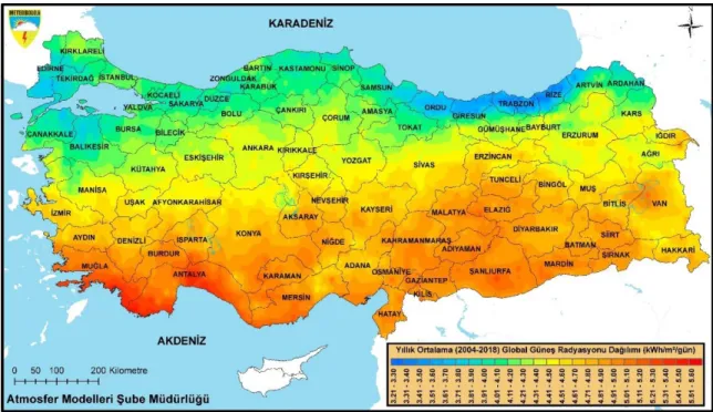
Figure 1.1: Solar radiation map of Turkey ... 2

Figure 2.1: The Multi-Criteria Decision Making classification. ... 5

Figure 2.2: Multi-Criteria Decision Making process. Source (Wang, Jing, Zhang, & Zhao, 2009) ... 8

Figure 2.3: The common system for MCDM analysis. (Kumar et al., 2017) ... 10

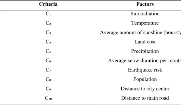
Figure 4.1: Turkey Sun Radiation Map ... 31

Figure 4.2: Earthquake Risk Map for Turkey ... 31

Figure 5.1: Unweighted and Weighted Supermatrix ... 54

Figure 5.2: Limit Supermatrix ... 54

Figure 5.3: Alternatives GAIA Plane ... 57

Figure 5.4: Criteria GAIA Plane ... 58

Figure 5.5: The GAIA Web of Mersin ... 60

Figure 5.6: The GAIA Web of Antalya ... 60

Figure 5.7: The GAIA Web of Konya ... 61

Figure 5.8: The GAIA Web of Isparta ... 61

Figure 5.9: The GAIA Web of Nigde ... 62

(9)

vii MCDM YÖNTEMLERİ KULLANARAK BİR GÜNEŞ ENERJİ SANTRALİ İÇİN EN İYİ KONUMU BULMAK İÇİN BİR FİZİBİLİTE ANALİZİ; TÜRKİYE'DE

BİR VAKA ÇALIŞMASI ÖZET

Güneş enerjisi, sürdürülebilir ve özgür bir karbon enerjisi geleceği için en iyi ve en umut verici yenilenebilir enerjilerden biri olarak kabul edilir. Bir güneş enerjisi santralinde, farklı faktörler sistem performansını etkileyebilir. Güneş enerjisi santralleri ile ilgili ana konulardan biri, tesisi kurmak için doğru lokasyonu seçmektir. Çalışma, Çok Kriterli Karar Verme (MCDM) yöntemini kullanarak Türkiye'deki bir güneş enerjisi santrali için en iyi konumu değerlendirmeyi ve seçmeyi amaçlamaktadır. Analizde Antalya, Mersin, Niğde, Isparta ve Konya olmak üzere beş farklı şehir dikkate alınmıştır. Güneş enerjisi santralinin performansını farklı faktörler etkileyebilir, bu çalışmada seçilen faktörler; alınan güneş radyasyonu ve güneş ışığı miktarı, sıcaklık, arazi maliyeti, nüfus, yağış, deprem riski, kar süresi ve ana yollara ve şehre yakınlıktır. merkez. MCDM, tüm hedefleri ve kriterleri aynı anda dikkate aldığı için enerji planlaması alanında karar vericilere yardımcı olan önemli bir araçtır. Kriterlere göre en iyi alternatifi belirlemek için üç iyi bilinen MCDM yöntemi Analitik Hiyerarşi Süreci (AHP), Analitik Ağ Süreci (ANP) ve zenginleştirme değerlendirmesi için Tercih sıralaması organizasyon yöntemi (PROMETHEE) kullanılır. Araştırmanın sonuçları, Mersin'in en iyi alternatif olduğunu ve ardından Antalya'nın diğer alternatiflerin her yönteme göre değişebileceğini, Niğde'nin ise en az tercih edilen alternatif olarak değerlendirildiğini göstermektedir.

Anahtar Kelimeler: Çok Kriterli Karar Verme, Yenilenebilir Enerji, Güneş enerjisi santrali, AHP, ANP, PROMETHEE

(10)

viii A FEASIBILITY ANALYSIS TO FIND THE OPTIMAL LOCATION FOR A SOLAR POWER PLANT BY USING MCDM METHODS; A CASE STUDY IN

TURKEY

ABSTRACT

Solar energy is considered one of the best and most promising renewable energy toward a sustainable and free carbon energy future. In a solar power plant, different factors can affect the system performance. One of the main issues related to solar plants is choosing the right location to install the facility. The study aims to evaluate and select the best location for a solar power plant in Turkey using Multi-Criteria Decision-Making (MCDM) method. Five different cities Antalya, Mersin, Nigde, Isparta, and Konya are considered in the analysis. Different factors might affect the performance of the solar power plant, in this study the selected factors are the amount of solar radiation and sunshine received, temperature, land cost, population, precipitation, earthquake risk, snow duration, and closeness to main roads and city center. MCDM is a significant tool that helps decision-makers in the field of energy planning since it considers all objectives and criteria at the same time. Three well-known MCDM methods Analytic Hierarchy Process (AHP), Analytical Network Process (ANP), and Preference ranking organization method for enrichment evaluation (PROMETHEE) are used to determine the best alternative according to the criteria. The results of the study demonstrate that Mersin is the best alternative followed by Antalya and the other alternatives might change according to each method, while Nigde scored the lowest score to be considered the least preferred alternative.

Keywords: Multi-Criteria Decision-Making, Renewable Energy, Solar power plant, AHP, ANP, PROMETHEE

(11)

1

1. INTRODUCTION

1.1 Study Topic

With the increasing number of population and trying to meet their needs, the energy consumption is increasing day by day. Humans started consuming energy since the day they seized to exist until our current day. There are many different forms of energy we use. There are the primary energy sources with two different categories first fossil fuels such as oil, natural gas, and coal and there is a different type of which is renewable resources including sun, wind, hydroelectric, and many different types. These resources also can be transformed into electricity, heat, and fuel which are essentials to our current lifestyle. Fossil fuels have many negative effects such as global warming and climate change, which cause an increase in the temperature of the whole world. Also, the use of fossil fuels causes pollution which might harm our health in many different ways air pollution might harm the respiratory system, also it will cause acid rains which will harm what we harvest and on us in general. Since our reliance on energy was most focused on fossil fuels, its resources and reserves are advancing at critical levels. People are trying to find new ways to rely on and use renewable resources since it is found in abandon and it doesn’t have the negative impacts on the environment like fossil fuels does, because of that its importance is increasing much more. Renewable energy is from a source that won’t deplete when used, it will renew itself and it can be used to reduce the progress of global warming and the depletion of the ozone layer. Solar energy is considered one of the best promising sources of renewable energy, it transforms the energy gained by the sun into electricity without the side effects caused by fossil fuel. Turkey is considered as a great option for renewable energy due to its significant location in terms of renewable energy capacity. Most of Turkey’s electricity demand is obtained through the use of fossil fuels. Turkey is located between 35 and 40 °N and 34 to 36 °E on the meridian, which implies that it is receiving a good amount of solar radiation especially during the summer, and compared to other developed countries Turkey is receiving a sufficient amount of average sunshine time. This makes Turkey a great option to use solar power if the optimal location

(12)

2 is selected to establish a solar power plant. Choosing the optimal location will make the solar power plant work with high efficiency which will provide both economical and environmental benefits.

1.2 Purpose of Thesis

This study aims to choose the best location to install a solar power plant in Turkey, most of the cities are receiving a good proportion of solar radiation. However, many other criteria affect the decision to choose the location along with the radiation amount. Firstly the criteria that impose greater effects on the location selection are determined, then different alternatives (cities) are chosen based on the amount of solar radiation they receive. Multi-Criteria Decision-Making (MCDM) is a branch related to operation research to obtain the optimal result in complex scenarios including different objectives, factors, constraints, and criteria. MCDM became popular in energy planning because it allows the decision-maker to consider all criteria and make decisions on the priorities by giving each criterion the desired weight accordingly. Analytic hierarchy process (AHP), analytic network process (ANP), and preference ranking organization method for enrichment evaluation (PROMETHEE) methods are used in this study.

(13)

3 As can be seen in figure 1.1, the southern part of Turkey is receiving a sufficient amount of solar radiation, which help to determine and choose the best alternatives. In this study, five cities (Antalya, Nigde, Mersin, Konya, and Isparta) are selected to be used in the analysis. These cities are chosen according to the amount of solar radiation received yearly. In addition to that, the best option or city to locate the solar power plant is then determined according to the gathered data for all the criteria and the results obtained by running the AHP, ANP, and PROMETHEE tests.

The following chapter, Literature review, demonstrates different researches and studies on ranking alternatives in different fields considering complex scenarios and factors. Furthermore, it also discusses the usage of Multi-Criteria Decision-Making methods in different studies and papers.

(14)

4

2. LITERATURE REVIEW

Academic literature contains many different methods and techniques that analyze and rank the alternatives in terms of qualitative and quantitative characteristics of different criteria within the alternatives. In the following study, a variation of projects, researches, and studies that are related to choosing the best alternative using MCDM methods are demonstrated.

A study about the solar energy performance in three different geographical locations in Turkey evaluated both project and cost-based wisely conducted by (Ozcan & Ersoz, 2019). The research describes how the photovoltaic system was implemented to evaluate the potential of solar energy in Turkey. The PV system was done for specific areas

occupying 180,330 m2 with a total of 8865 MW installed power of the system. Based on

the obtained results Izmir had more efficient results regarding the performance to produce electricity than Ankara and Istanbul, making it the best alternative to invest in.

2.1 Multi-Criteria Decision-Making (MCDM)

Making a decision while taking into consideration different opposing factors is known as multiple criteria decision making (MCDM). Decision making is an essential activity to make throughout every day. Everyday life consists of MCDM problems. When buying a personal thing such as a house or a car, the individual should consider some factors such as price, size, style, safety, comfort, etc. In a different aspect, business MCDM problems are more complicated and usually of large scale. To acquire different departments of large companies, the evaluation of their supplier through different factors is required such as sale service, quality management, financial stability, etc. for instance, many companies in Europe conduct organizational self-assessment using many criteria and sub-criteria sets, to match the EFQM (European Foundation for Quality Management) business excellence model. The development of computer technology has a huge impact on the progress of MCDM. MCDM importance is increasing in supporting business decision making,

(15)

5 because the usage of computer and information technology is increasing worldwide, creating an immense amount of information to consider for decision making (Xu & Yang, 2001).

In today’s ultra-modern world, to choose and make the right and effective decision is an important action to perform. Decision-making is the act to choose the right decision according to the preferences set by the decision-maker(s) between one or many sets of alternatives. Multi-criteria decision-making is a theory designed in the early seventies, to deal with complex and rational decision-making problems, taking into consideration multiple different criteria simultaneously. Later on, the MCDM was developed at the same time as the uncertainty and chaos theory development. Zadeh introduced the uncertainty of the fuzzy set theory that was accepted by MCDM supporters. Fuzzy MCDM is a new decision theory created by mixing MCDM and fuzzy set theory by Carlsson and Fuller, this new method has been useful in many different applications in the real world (Abdullah, 2013).

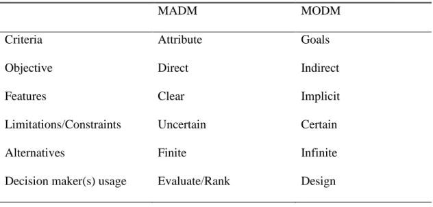
The study done by (Sabaei, Erkoyuncu, & Roy, 2015) express the importance of understanding the decision-making classifications to select an appropriate method. MCDM can be easily classified according to the number of answers whether it's infinite or finite as shown in Table 2.1. In general, all MCDM methods can be divided into two main groups Multi-Attribute Decision Making (MADM) and Multi-Objective Decision Making (MODM).

Figure 2.1: The Multi-Criteria Decision Making classification.

Multi-Criteria Decsion

Making

Multi Attribute Decision

Making (MADM)

Multi Objective Decision

Making (MODM)

(16)

6 Figure 2.1 shows the classification of MCDM, Multi-Attribute Decision Making (MADM), and Multi-Objective Decision Making (MODM). Even though both groups have similar characteristics, they also have different features. Table 2.1 shows the difference between the two methods, for example, it demonstrates how MADM considers a limited number of alternatives because of this prioritizing become more difficult so the final result is ranked according to the comparison of alternatives considering each criterion considered. Whereas the MODM evaluates ongoing alternatives with a limitless number of possible values of the outcome, to enhance the objective functions, the constraints are taken into consideration while reducing the performance of other objectives. Also, MADM preference depends on the set of features, while MODM depends on the set of objectives given (Kumar et al., 2017).

Table 2.1: Comparison between MADM and MODM

MADM MODM

Criteria Attribute Goals

Objective Direct Indirect

Features Clear Implicit

Limitations/Constraints Uncertain Certain

Alternatives Finite Infinite

Decision maker(s) usage Evaluate/Rank Design

In this step, the process of solving MCDM problems is described and demonstrated in figures 2.2 and 2.3:

(a) Define the objective

Define the goal or the aim of the problem.

(b) Select the appropriate alternatives and criteria

The alternatives are chosen based on the performance expected regarding the objective, while the criteria selected depends on the impact of the factors on the performance of the

(17)

7 alternatives. The alternatives selected are based on the decision-makers’ preferences or sometimes based on information collected from different sources such as literature studies and papers.

(c) Criteria weighting

One of the most important and difficult phases of MCDM problems is to choose the criteria weight. The weight of criteria is determined based on the decision-makers’ perspective and how the selected criteria might may have an impact on the alternative performance. It can be calculated in different ways, but always the sum of weights should be equal to one so the alternatives could be compared with each other with the desired set of criteria. The weight can be calculated in some problems, be given by specialists, or obtained from published literature studies.

(d) Evaluation

MCDM consists of many different methods, according to available data and the decision-making problem the right MCDM will be determined to implement in the problem. (e) Final calculations to obtain the rank

When the method is determined, it can easily be used to calculate the results and find the best alternative for the decision-makers by ranking the alternatives from the most to least preferred accordingly.

(18)

8 Figure 2.2: Multi-Criteria Decision Making process. Source (Wang, Jing, Zhang, &

(19)

9 Based on figure 2.2, the decision-making process is divided into three steps methods of selection of criteria, determining the weights of the criteria, and rank the alternatives. The first step consists of establishing the goal, find suitable alternatives, and determine the criteria that have an impact on the performance of the alternative. The following step criteria weighting is to determine the importance of each criterion by giving it a weight. After assigning the weight for each criterion, MCDM methods will be applied to select and rank the best alternative. In the last step, the process will come to end in case the order of the ranked alternatives is the same as other MCDM methods, otherwise, if there is a significant difference the ranking results will be calculated again until the best scenario is determined (Wang et al., 2009).

(20)

10 Figure 2.3: The common system for MCDM analysis. (Kumar et al., 2017) Figure 2.3 demonstrates a general system to solve MCDM problems, each problem can be approached by different methods based on the objective defined, functions selected, and the one that deals with the criteria in a better way. Each method has its way and constraints, but figure 2.3 explains express the main general steps to be able to solve the decision problem (Kumar et al., 2017).

The research done by (Sánchez-Lozano, García-Cascales, & Lamata, 2015) explains how the selection of the optimal location to install a solar power plant is determined by evaluating the suitable locations. The article explains that a combination of GIS tools and MCDM methods is one of the best ways to solve complicated location decision problems. The research narrows down the locations by eliminating the restricted and protected areas, and the criteria that affect the decision making.

Start

Establish objective/goal

Select criteria that will have an impact on the problem

based on objectives

Select alternatives that best satisfy the need of the

objective

Determine the weights/priority for

alternatives

Select the best MCDM method for the objective

Find the optimal alternative

Acceptable

(21)

11 In another research done by (Sozen, Mirzapour, & Çakir, 2015) the best location for a solar power plant in Turkey is determined. In this study, the geographical and environmental factors linked to solar power are examined. The article aimed to find the best location, using data gathered from data envelopment analysis (DEA) for 12 months. They used the TOPSIS method and concluded that among 30 different alternatives (cities) the optimal location is Nigde. Another review of renewable energy development using MCDM methods done by (Kumar et al., 2017) discusses how decision-makers may feel restricted due to the limitations they face when trying to optimize the energy alternatives. Energy planning has become difficult due to the combination of different criteria like social, technical, economic, and environmental. To help the decision-makers make better decisions, the research implies the use of the MCDM method. MCDM is a branch of operation research that helps the decision-makers to find the optimal results in complicated frameworks such as conflicting objectives and constraints, and it allows them to deal with each constraint to help them to determine the optimal outcome. Because of its resilience, MCDM tools are becoming popular in the energy planning sector, since it allows the decision-makers to consider their criteria and take decisions at the same time. Three MCDM methods are selected to be applied in this study. They are Analytic Hierarchy Process (AHP), Analytic Network Process (ANP), and The preference ranking organization method for enrichment evaluations (PROMETHTEE). In the following section, the selected MCDM methods, their steps, and the fields they are applied to are described.

2.1.1 Analytic hierarchy process (AHP)

The analytic hierarchy process (AHP) was introduced by Thomas L. Saaty in the 1970s. AHP is an MCDM method that analyzes and evaluates complex decisions based on mathematics and psychology (factors that have an impact on the alternatives). AHP doesn’t help the decision-makers to make the correct decision, but instead, it helps them to understand the problem and find the best alternative to satisfy their goal. The research done by (Emrouznejad & Marra, 2017) explains that AHP allows decision-makers to evaluate complex alternatives with different characteristics. AHP is considered more advanced than other MCDM methods because it deals with subjective indicators. AHP is

(22)

12 used in a significant way, the evaluation of the alternative is subjective and it deals with multiple criteria problems. AHP is used worldwide in different fields regarding decision-making problems. For instance, the research done by (Al-Subhi Al-Harbi, 2001) demonstrates how the implementation of AHP in project management to select the best contractor that prequalifies the project. A hierarchal model was built including priorities and indicators according to the owner preferences and prerequisites also the individual’s characteristics of the contractors were taken into consideration.

Another field AHP was used in is selecting the best water supply source done by (Ihimekpen & Isagba, 2017) the research was conducted for Benin city. Four major water supply sources were selected for this study, and considering the following criteria cost, availability, accessibility, sustainability, quality, and ease of access. After the application of AHP, groundwater scored the highest score of 0.4130 making it the best water supply for Benin City.

One of the famous fields AHP is used in is site selection, in the research done by (Ozdemir & Sahin, 2018) AHP was used to find the optimal location for a solar PV power plant among three local regions in turkey. In this study, the problem was approached in two ways. First, to acquire the exact amount, the amount of electricity produced is measured. After that, the decision-maker provide linguistic data that will be used. According to the results acquired, Kulluk was considered the best location to install the PV power plant. The research done by (Anderluh, Hemmelmayr, & Rüdiger, 2020) to select the best location for a city hub in Vienna. In this study, a medium-sized city hub was selected and three stakeholder parties were considered. AHP model was established to find the optimal location considering both quantitative and qualitative criteria. The results show that AHP can achieve a good comprise between the stakeholder parties.

A study using the GIS-AHP approach to select the best site for a solar PV power plant in Saudi Arabia done by (Al Garni & Awasthi, 2017) suggests that the optimal areas to locate a solar plant are in the north and northwest of Saudi Arabia. Using GIS and MCDM methods and taking into consideration the different factors that will have an impact on the plant performance. The preferred areas had the following motif, approximately near to transmission lines, urban areas, and main roads.

(23)

13 Another research done by (Baswaraj, Sreenivasa Rao, & Pawar, 2018) the application of AHP to select the process parameters and check the consistency for a secondary steel production. This study aims to focus on improving the parameters for steel recycling, for Indian steel recycling industries using AHP. Five requirements to increase the strength properties of secondary steel have been established. The key contribution to the industry is quality improvement in secondary steel production. To assure the quality, AHP model was established, which allows the fusion of tangible and intangible requirements, check the consistency, and helps enhance the secondary steel recycling industries.

In the research done by (Di Angelo, Di Stefano, Fratocchi, & Marzola, 2018) an AHP-based method was applied to select the best 3D cultural heritage scanner. AHP is used in this research to be able to construct this choice since there is no 3D scanner that matches all the requirements the choice would be carried out in an unstructured manner. The implementation AHP method in two different circumstances regarding pottery fragments emphasizes its ease of use, the complexity confirmed by the consistency check. Taking relevant factors into consideration, the accuracy of the technical and economic assessment was determined. Combining the competencies it would be possible to apply it in different fields such as archaeology and 3D digital devices in a structured manner.

A study using the combination of AHP and TOPSIS methods to determine the best location for a solar power plant in turkey was performed by (Akçay & Atak, 2018) to discuss that many criteria will affect the decision making. In this study, the main criteria and sub-criteria are determined according to the factors that might affect the decision making of the best location. The best location determined was Mersin among the alternatives according to the AHP and TOPSIS method.

A study for a group decision making to choose the best location for a facility was conducted by (Kahraman, Ruan, & Doǧan, 2003). The study aims to solve a facility location problem using four different approaches of fuzzy multi-attribute group decisions including AHP. The research shows how qualitative and quantitative criteria were taken into consideration. The result of the study shows that with 0.47 as a final score Izmir is the best option compared to the other alternatives.

(24)

14 2.1.2 Analytic network process (ANP)

The analytic network process (ANP) was developed by Thomas L. Saaty in 1996. Similar to AHP, ANP uses a system of pairwise comparison to define the weight of the criteria, check the consistency, and rank the alternatives. ANP differs from AHP since it doesn’t require independence between the factors because real-life decision problems consist of interdependency between the factors and the alternatives which make ANP a successful method to use. According to (T. L. Saaty, 2006) many decision problems can’t be solved using hierarchical structure because they include higher-level factors that interact and depend on lower-level elements in a hierarchy model. Thus, instead of hierarchy, a network is used to represent ANP. The ANP structure looks like a network, and the component and elements are connected by nodes. The origin of the path can be described as a source node, while the sink node is the destination of the importance of the paths and can never be the root of the mentioned paths. For instance, the research done by (Gencer & Gürpinar, 2007) to select the best supplier in an electronic firm case study, consider the factors to evaluate the best supplier since it is a crucial factor for business success in today’s competitive market. In this study, the criteria were established based on the structure of the business movement and was applied in a real case study. The best supplier alternative ranked in ANP was also approved by the purchasing manager.

Another research done by (Hosseini, Tavakkoli-Moghaddam, Vahdani, Mousavi, & Kia, 2013) to evaluate and select the best strategy to minimize the risks in a supply chain. The study considers four well-known types of risks in the supply chain (SC). To reduce the risk a good strategy must be adopted, therefore, five alternatives were selected. A new supply chain network was established and ANP was applied. According to the result acquired using ANP, total quality management (TQM) with a score of 0.483 was selected as the best strategy among the other alternatives.

The research was done by (Agarwal, Shankar, & Tiwari, 2006) to model lean, agile, and legible supply chain metrics using an ANP-based approach. The paper aims to discover the relationship between the criteria including lead time, cost, quality, and service level, and the alternatives lean, agile, and legible for a fast-moving consumer good business in a supply chain (SC) case. According to ANP, the leanness SC increase the profit by

(25)

15 reducing the cost, while agility provides what the customer exactly needs with no extra cost to increase the profit. The legible SC allows the downstream part to acquire high service levels while the upstream part of the network to be cost-effective.

Another research done by (Hu, Hoare, Raftery, & O’Donnell, 2019) about environmental and energy efficiency evaluation of buildings using the ANP-based approach. The study aims to provide a better understanding of the building managers using improved environmental and energy performance evaluation by combining scenario modeling with Fuzzy ANP. The method was applied for a case study where the sports center scored an operational score of 56.9 out of 100 (i.e. very good) in terms of operational performance considering eight selected factors.

Research done by (Simwanda, Murayama, & Ranagalage, 2020) talks about the change of drivers of urban land use in a case study done in Lusaka, Zambia using an ANP approach. The study aims to select one of six urban areas in Lusaka, considering different factors. The results expressed that some factors are the major drivers of urban-LU, for example socio-economic (55.11%) and population (27.37%). The ANP model ranked unplanned high-density residential (UHDR) as the best alternative followed by the commercial and industrial (CMI) areas as the fastest-growing driven by the relation with other factors. Furthermore, the study suggests several strategies to improve the policies of urban planning.

2.1.3 The preference ranking organization method for enrichment evaluations (PROMETHTEE)

The preference ranking organization method for enrichment evaluations

(PROMETHTEE) basic elements were introduced by Professor Jean-Pierre Brans in 1982. Then it was developed and extended by (Brans, Vincke, & Mareschal, 1986). Similar to other MCDM methods, PROMETHEE is considered as an outranking method, it provides decision-makers the opportunity to control the difference between the criteria and reduce the effort required to create a preference model. Outranking methods allow the decision-makers to deal with real decision problems, to describe the problem better, and to perform sensitivity analyses. Outranking methods are considered as successful methods due to their mathematical properties and the ability to deal with imperfect criteria, these methods

(26)

16 can be applied in many fields. PROMETHEE demonstrates the importance of each criterion compared to the alternatives. For instance, the research done by (Huth, Drechsler, & Köhler, 2005) focuses on the evaluation of harvesting methods using PROMETHEE since each alternative has different characteristics including both qualitative and quantitative data.

PROMETHEE is applied in many fields, it was used in is social sustainability assessment of composting technologies done by (Makan & Fadili, 2020) in the field of social sustainability. The purpose of the research is to evaluate and rank the suitable technology to use in composting. Taking into consideration the performance of the alternative to each criterion, the obtained results demonstrate that the reactor technologies are more sustainable than enclosed technologies.

Another field PROMETHEE was used in is water resource planning done by (Abu-Taleb & Mareschal, 1995) in water resource development. PROMETHEE handles the connections and the variability between the factors for water resource development problems. The factors used in this study are environmental protection, water demand and supply management, and regional cooperation.

Research done by (Hokkanen & Salminen, 1997) about environmental assessment dealing with a problem of locating a waste treatment facility in eastern Finland. The research discusses how the implementation of PROMETHEE was a success and has changed the decision-makers' opinions from being based on a single point of view in the beginning into broad debates considering all points of view.

In another case done by (Hermans, Erickson, Noordewier, Sheldon, & Kline, 2007) PROMETHEE is used to rank different river management alternatives for the Upper White River of Central Vermont, in the northeastern United States. The stakeholders’ discussion was improved after using the PROMETHEE method, it allowed them to think beyond the river management alternatives but also to study how they can use the alternatives efficiently on the rivers range.

Another research to select a green supplier using the PROMETHEE method is done by (Abdullah, Chan, & Afshari, 2019). The research aims to select the best green supplier

(27)

17 among different groups of alternatives using the usual preference function. Using the PROMETHEE algorithm, the research implies that supplier A1 is the most favorite alternative, although different preference functions were used later again supplier A1 was the best alternative.

(28)

18 Table 2.2: The selected MCDM methods used in different fields.

Method Area of Application Authors

AHP Evaluating and Ranking (Rosenbloom, 1997)

(Leung & Cao, 2000) (Kang & Lee, 2007)

(Sinuany-Stern, Mehrez, & Hadad, 2000)

Location Selection (Sennaroglu & Varlik

Celebi, 2018) (Ka, 2011)

(Hosseini et al., 2013)

(Mousavi,

Tavakkoli-Moghaddam, Heydar, & Ebrahimnejad, 2013)

ANP Financial Management (Akhisar, 2014)

(Hasan, Ümit, & Serhat, 2016)

(Reza & Majid, 2013)

Evaluating and Ranking (Dou, Zhu, & Sarkis, 2014)

(Poonikom, O’Brien, & Chansa-ngavej, 2004) (Sevkli et al., 2012)

(Chung, Lee, & Pearn, 2005)

(29)

19

Table 2.2 (Continued).

PROMETHEE Water Management (Hajkowicz & Higgins,

2008)

(Hyde & Maier, 2006) (Fontana & Morais, 2016)

Financial Management (Kalogeras, Baourakis,

Zopounidis, & Van Dijk, 2005)

(Doumpos & Zopounidis, 2004)

(De Smet & Guzmán, 2004) (Albadvi, Chaharsooghi, & Esfahanipour, 2006)

Outranking (Vaillancourt & Waaub,

2002)

(Vego, Kučar-Dragičević, & Koprivanac, 2008)

(Spengler, Geldermann,

Hähre, Sieverdingbeck, & Rentz, 1998)

The next chapter will explain the three selected MCDM methods for this study, the procedures and steps will be discussed and shown.

(30)

20

3. METHODOLOGY

3.1 Analytic Hierarchy Process (AHP)

Another MCDM useful method is AHP, decision-makers can make better decision considering different factors. Thomas Saaty (1980) introduced the Analytic Hierarchy Process (AHP), which is considered an effective method because it allows the decision-makers to define their priorities by dealing with complex situations. AHP aims to consider the best decision concerning subjective and objective angles, by transforming the complex decisions into a sequence of pairwise comparisons and synthesize the results. Checking the consistency is another technique that AHP integrates, allow the DMs to make a better decision (Moutinho, Hutcheson, & Beynon, 2014).

Step 1: Develop the weights of criteria Step 1.1 Create a pairwise decision matrix.

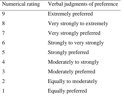
Table 3.1: Pairwise Comparison Scale. Source: (R. W. Saaty, 1987)

Numerical rating Verbal judgments of preference

9 Extremely preferred

8 Very strongly to extremely

7 Very strongly preferred

6 Strongly to very strongly

5 Strongly preferred

4 Moderately to strongly

3 Moderately preferred

2 Equally to moderately

(31)

21 The chosen alternatives and criteria will be demonstrated in a decision matrix form, as shown below. Assume i=1, 2……, m j=1, 2……, n Matrix: 𝐴 = ( 𝑥11 𝑥12 … 𝑥1𝑛 𝑥21 𝑥22 … 𝑥2𝑛 𝑥_𝑚1 𝑥_𝑚2 … 𝑥_𝑚𝑛) (1)

Step 1.2: There are many different ways to normalize the data collected from different sources. To compare the data from different sources, the data should be normalized. In this study, the matrix was normalized by finding the sum of each column, after that each value will be divided by the total respectively. The following equation is used to find the sum for each column.

𝑆_𝑛 = ∑ 𝑎_𝑗𝑖 𝑘−1 𝑗=1 𝑤ℎ𝑒𝑟𝑒 𝑘 = 𝑛 + 1, 𝑖 = 𝑛 (2) 𝐵 = ( 𝑛₁₁ 𝑛₁₂ … 𝑛_1𝑛 𝑛21 𝑛22 … 𝑛2𝑛 𝑛𝑚1 𝑛𝑚2 … 𝑛𝑚𝑛 )

Then find the priority vector, normalize the result acquired by the nth_{to get the proper}

weight. To normalize the nth root will be divided by the sum of all nth root, for each criterion

individually. Normalizing can be referred to priority vector, which will be obtained by this function:

𝑃𝑉 =∑ 𝑟𝑗

𝑛 (3)

Step 1.3: Calculate and check the consistency ratio (CR)

According to (Bozóki & Rapcsák, 2008) pairwise comparison matrices are rarely stable in real-life situations, because of that decision-makers try to achieve a better level of

(32)

22 consistency considering the decisions made on inconsistent data may be meaningless. Saaty (1980) proposed the formula for calculating inconsistency.

Step 1.3.1: Calculate the consistency measure (CM)

The general equation used to calculate the consistency measure is:

𝐶𝑀_𝑗 =𝑅𝑗× 𝑃𝑉

𝑃𝑉_𝑗 𝑤ℎ𝑒𝑟𝑒 𝑗 = 1,2,3 … 𝑛 (4)

Rj corresponds to the row comparison of the matrix, and PVj represents the corresponding

element in PV.

Step 1.3.2: To calculate the consistency ratio, first the consistency index (CI) should be calculated. The average consistency measure vector determined in the previous step

isλ_𝑚𝑎𝑥 − 𝑛. The consistency index is obtained using the formula below.

𝐶𝐼 = λ𝑚𝑎𝑥− 𝑛

𝑛 − 1 (5)

After calculating the result of the consistency index, the random index (RI) can be obtained from table 3 the random index table done by Saaty.

Step 1.3.3: The formula used to calculate the consistency ratio is shown below:

𝐶𝑅 = 𝐶𝐼

𝑅𝐼 (6)

Step 2: Develop the rating for each decision alternative for each criterion by:

Step 2.1: Developing a pairwise comparison matrix for each criterion, with each matrix containing the pair-wise comparisons of the performance of decision alternative on each criterion;

(33)

23 Matrix: 𝐴 = ( 𝑥₁₁ 𝑥₁₂ … 𝑥_1𝑛 𝑥21 𝑥22 … 𝑥2𝑛 𝑥𝑚1 𝑥𝑚2 … 𝑥𝑚𝑛 ) (7)

Step 2.2: Normalizing the aforementioned nth root of the product values to get the corresponding ratings; 𝐵 = ( 𝑛₁₁ 𝑛₁₂ … 𝑛_1𝑛 𝑛₂₁ 𝑛₂₂ … 𝑛_2𝑛 𝑛𝑚1 𝑛𝑚2 … 𝑛𝑚𝑛 ) (8)

Step 2.3: Calculating and checking the Consistency Ratio (CR)

Step 2.3.1: To calculate the consistency ratio, first the consistency index (CI) should be determined. The consistency index shows the consistency of judgments across all pairwise comparisons. The consistency index is obtained using the formula below.

𝐶𝐼 = λ𝑚𝑎𝑥− 𝑛

𝑛 − 1 (9)

After calculating the result of the consistency index, the random index (RI) can be obtained from the random index table done by Saaty.

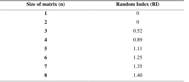
Table 3.2: Random index table (source: (T. L. Saaty & Tran, 2007))

Size of matrix (n) Random Index (RI)

1 0 2 0 3 0.52 4 0.89 5 1.11 6 1.25 7 1.35 8 1.40

(34)

24 Step 2.3.2: The formula used to calculate the consistency ratio is shown below:

𝐶𝑅 =𝐶𝐼

𝑅𝐼 (10)

Step 3: Final step is to calculate the weighted average rating for each decision alternative, according to the results, the alternative with the highest score is considered as the best option. To calculate the final score for each alternative, the criteria weights obtained from step 1 will be multiplied by the ratings obtained from step 2 and sum them up respectively.

3.2 Analytical Network Process (ANP)

Multi-criteria decision making has different methods, but one of the most advanced methods is Analytical Network Process (ANP). ANP is one of the best methods to make decisions in real-life problems because it provides the relation and dependence between elements of both the alternative and criteria in the model (Kadoi et al., n.d.).

Step 1: Create a pairwise comparison matrix:

𝐴 = (

𝑥₁₁ 𝑥₁₂ … 𝑥_1𝑛

𝑥₂₁ 𝑥₂₂ … 𝑥_2𝑛

𝑥_𝑚1 𝑥_𝑚2 … 𝑥_𝑚𝑛)

(11)

Step 2: Normalize the matrix:

There are many different ways to normalize the data collected from different sources. To compare the data from different sources, the data should be normalized. In this study, the matrix was normalized by finding the sum of each column, after that each value will be divided by the total respectively. The following equation is used to find the sum for each column. 𝑆𝑛 = ∑ 𝑎𝑗𝑖 𝑘−1 𝑗=1 𝑤ℎ𝑒𝑟𝑒 𝑘 = 𝑛 + 1, 𝑖 = 𝑛 (12)

(35)

25 𝐵 = (

𝑛₁₁ 𝑛₁₂ … 𝑛_1𝑛

𝑛₂₁ 𝑛₂₂ … 𝑛_2𝑛

𝑛_𝑚1 𝑛_𝑚2 … 𝑛_𝑚𝑛)

After calculating the total each value will be divided with the result. For example:

𝑛₂₁= 𝑥21

𝑆_𝑛 (13)

Step 3: Check the consistency.

Three consistency metrics are used for this method consistency measure (CM), consistency index (CI), and consistency ratio (CR) to assure the reliability of the pairwise comparison.

Step 3.1: Consistency Measure (CM)

The general equation used to calculate the consistency measure is:

𝐶𝑀_𝑗 =𝑅𝑗× 𝐸𝑉

𝐸𝑉_𝑗 𝑤ℎ𝑒𝑟𝑒 𝑗 = 1,2,3 … 𝑛 (14)

Rj corresponds to the row comparison of the matrix. While EV refers to Eigenvector which

is also known as the priority vector, and EVj represents the corresponding element in EV.

Step 3.2: Consistency Index (CI)

The average consistency measure vector determined in the previous step isλ_𝑚𝑎𝑥− 𝑛. As

explained in the previous method the consistency index is calculated by the equation below:

𝐶𝐼 =λ𝑚𝑎𝑥 − 𝑛

𝑛 − 1 (15)

Step 3.3: Consistency Ratio (CR)

(36)

26

𝐶𝑅 =𝐶𝐼

𝑅𝐼 (16)

Step 4: Sensitivity analysis

The stability of alternatives ranking is recommended to be checked by performing the sensitivity analysis. The obtained results through the ANP model are analyzed by the sensitivity analysis. It shows the relation between the elements of alternatives and criteria, where the element of criteria has an impact on the elements of alternatives and vice versa (Farman et al., 2017).

Step 5: After finding the consistency ratio and performing the sensitivity analysis test, the alternatives will be ranked from the most to least preferred.

3.3 Preference ranking organization method for enrichment evaluation (PROMETHEE)

One of the MCDM methods used to solve the decision-making problem is PROMETHEE. In this method, all alternatives will be compared to each criterion. Then a specific preference functions in PROMETHEE is used to show the differences in the preference of each alternative with respect to each criterion. The preference functions have a range from 0 to 1 and it is assigned according to the decision-maker point of view. If the range is close to 1 it means it there is a large difference in the preference of the alternatives. On the other hand, range 0 describes that there is no difference in preference between the compared alternatives.

Step 1: Create a decision matrix.

The chosen alternatives and criteria will be demonstrated as xij in a decision matrix form,

as shown below. The alternatives will be demonstrated as i and j represents the criteria. Assume i=1, 2……, m

(37)

27 Matrix: 𝐴 = ( 𝑥₁₁ 𝑥₁₂ … 𝑥_1𝑛 𝑥21 𝑥22 … 𝑥2𝑛 𝑥𝑚1 𝑥𝑚2 … 𝑥𝑚𝑛 ) (17)

Step 2: Determine the weight wj of the criteria. To demonstrate the importance of each

criterion.

∑ 𝑤𝑗 = 1

𝑘

𝑗=1

(18)

Step 3: Normalize the matrix created.

There are many different ways to normalize the data collected from different sources. To compare the data from different sources, the data should be normalized. In cases where decision-makers need to rate and rank their decisions, the matrix should be normalized. Consider the data as a vector when normalized its magnitude will change but the direction stays the same. In other words normalizing is performed to make the different data obtained similar so it can be compared. In this study, the following equation is used to normalize the matrix.

[𝑥𝑖𝑗 − min (𝑥𝑖𝑗)] [max(𝑥_𝑖𝑗) − min (𝑥_𝑖𝑗)] ₍₁₉₎ 𝐵 = ( 𝑛11 𝑛12 … 𝑛1𝑛 𝑛21 𝑛22 … 𝑛2𝑛 𝑛_𝑚1 𝑛_𝑚2 … 𝑛_𝑚𝑛 )

Xij represents the alternatives i=1, 2…, m, while the criteria are represented by j=1, 2…,

n

Step 4: Make a pairwise comparison.

It is a process to compare the alternatives to determine which alternative is preferred and whether are the alternatives similar or not.

(38)

28 PROMETHEE has six preference functions that range from 0 to 1. In this research, the usual function is selected since there is no need for any parameter.

The usual function:

𝑃(𝑥) = 0 𝑖𝑓 𝑥 ≤ 0 (20)

𝑃(𝑥) = 1 𝑖𝑓 𝑥 > 0 (21)

Step 6: Rank the preference order by measuring the positive and negative outranking flow. The positive outranking flow is also represented as the leaving flow, and the negative outranking flow is also represented as entering flow. The leaving flow describes the strength of the alternative, on the other hand, the entering flow describes the weakness of the alternative.

The leaving flow:

∅+_{(𝑎) =} 1

𝑛 − 1∑ 𝜋(𝑎, 𝑥)

𝑥∈𝐴

(22)

The entering flow:

∅−_{(𝑎) =} 1

𝑛 − 1∑ 𝜋(𝑎, 𝑥)

𝑥∈𝐴

(23)

Step 7: In this step, the obtained entering and leaving flow will be used to calculate the alternatives outranking net flow using the following formula:

∅(𝑖) = ∅+_{− ∅}−_(𝑖) ₍₂₄₎

Step 8: Finally the alternatives will be ranked from the most to least preferred according to the net flow results obtained.

(39)

29 Table 3.3: The formulas used for Each Method

AHP ANP PROMETHEE

𝑆𝑛 = ∑ 𝑎𝑗𝑖 𝑘−1 𝑗=1 𝑘 = 𝑛 + 1, 𝑖 = 𝑛 𝑆𝑛 = ∑ 𝑎𝑗𝑖 𝑘−1 𝑗=1 𝑘 = 𝑛 + 1, 𝑖 = 𝑛 ∑ 𝑤𝑗 = 1 𝑘 𝑗=1 𝑘 = 𝑛 + 1, 𝑖 = 𝑛 𝑃𝑉 =∑ 𝑟𝑗 𝑛 𝐸𝑉 = ∑ 𝑟𝑗 𝑛 [𝑥𝑖𝑗 − min (𝑥𝑖𝑗)] [max(𝑥_𝑖𝑗) − min (𝑥_𝑖𝑗)] 𝐶𝑀_𝑗 = 𝑅𝑗 × 𝑃𝑉 𝑃𝑉_𝑗 𝑗 = 1,2,3 … 𝑛 𝑗 = 1,2,3 … 𝑛 𝐶𝑀_𝑗 =𝑅𝑗 × 𝐸𝑉 𝐸𝑉_𝑗 𝑗 = 1,2,3 … 𝑛 𝑗 = 1,2,3 … 𝑛 P(x) = 0 if x ≤ 0 P(x) =1 if x > 0 𝐶𝐼 =λ𝑚𝑎𝑥 − 𝑛 𝑛 − 1 𝐶𝐼 = λ_𝑚𝑎𝑥− 𝑛 𝑛 − 1 ∅ +_{(𝑎) =} 1 𝑛 − 1∑ 𝜋(𝑎, 𝑥) 𝑥∈𝐴 𝐶𝑅 =𝐶𝐼 𝑅𝐼 𝐶𝑅 = 𝐶𝐼 𝑅𝐼 ∅ −_{(𝑎) =} 1 𝑛 − 1∑ 𝜋(𝑎, 𝑥) 𝑥∈𝐴 ∅(𝑖) = ∅+− ∅−(𝑖)

In the following chapter, the data collection is demonstrated. The sources data were collected from, the alternatives, and the criteria used in this problem.

(40)

30

4. DATA COLLECTION

According to various researches and articles that are stated in the literature review, it helped to understand and select the right factors that have the most impact related to this case study. For each factor, sufficient data was collected from the following databanks.  TR MINISTRY OF INTERIOR: Department of Earthquake

 General Directorate of Meteorology  World Weather Online

 Gaisma.com  Weather Spark

Gathering the information for 12 months from these sources and monitoring the factors related to our research make it easier to understand and determine the alternatives and criteria to work with. According to the data gathered regarding the solar radiation, it narrowed it down to five cities in turkey and ten criteria.

(41)

31 Figure 4.1: Turkey Sun Radiation Map

4.1 Cities (Alternatives)

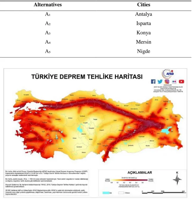
The reason the cities selected in Table 4.1 is that they receive a sufficient amount of solar radiation year-round, have a high temperature and have a high average of sun hours per day. In this study the alternatives are the selected cities Antalya, Mersin, Nigde, Konya, and Isparta are the alternatives.

Table 4.1: Selected Cities (Alternatives)

Alternatives Cities A₁ Antalya A₂ Isparta A₃ Konya A₄ Mersin A₅ Nigde

(42)

32 Figure 4.2 demonstrates the earthquake risk for Turkey, the areas with dark red have higher risk of earthquake compared to the areas expressed in lighter color or yellow. 4.2 Factors (Criteria)

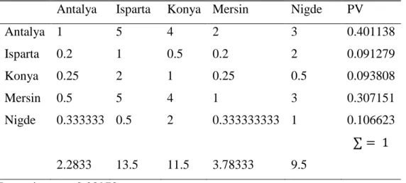
Choosing the right factors is an essential step to get better and more accurate results. Choosing the factors to allow the decision-maker to make better comparisons, by comparing the same factor of a city concerning the same factor of another city will help to understand which city is more efficient according to the specific factor. In this research, the factors shown in Table 4.2 were selected based on researches done to similar studies and articles.

Table 4.2: Criteria

Criteria Factors

C₁ Sun radiation

C₂ Temperature

C₃ Average amount of sunshine (hours/year)

C₄ Land cost

C₅ Precipitation

C₆ Average snow duration per month

C₇ Earthquake risk

C₈ Population

C₉ Distance to city center

(43)

33 Table 4.3: Collected data from sources.

C1 C2 C3 C4 C5 C6 C7 C8 C9 C1 0 A1 5089 18.6 3072 697 1009 0 0 2,364,00 0 8.04 4.0 A2 4995 19 2718 261 655 0 1.15 1,749,00 0 1.49 0.5 A3 4753 11.3 2693 76 337 3.7 1.05 2,180,00 0 6.8 1.75 A4 4787 10.8 2521 795 338 4.2 1.4 352.727 1.9 1.3 A5 4748 11.9 2713 60 537 3.6 1.66 433,830 7.5 1.0

(44)

34

5. RESULTS AND DISCUSSION

The results computed from the data obtained using different methods are presented in this chapter. The collected data were first calculated accurately using AHP and ANP in a program called super decision. After that, the data was calculated again using the third method PROMETHEE in a different program called Visual PROMETHEE.

5.1 AHP

The following steps can be calculated either manually or automatically by the Super Decision software:

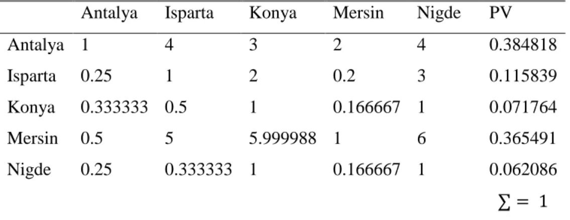
In this study, the application Super Decision was used to find the optimal alternative. AHP can be solved manually or using such applications. The usage of such applications is useful since it gives more accurate results with less time. The following procedure explains the AHP steps and how it can be done manually or automatically by the software: 1. Synthesizing the pair-wise comparison matrix is d by dividing each element of the matrix by its column total. For example, the value 0.43796 in table 5.2 is obtained by dividing 1 from table 5.1 by 2.2833, the sum of the same column from table 5.1 (1+0.2+0.25+0.5+0.333333).

2. Priority vector can be calculated by finding the row averages of the synthesized matrix. For example, the priority vector of Antalya is obtained by calculating the total of the first row (0.43796+0.37037+0.34783+0.52863+0.31579) and divide the result by the number of the alternatives, i.e. 5 to obtain the value. The priority vector for solar radiation (C1) demonstrated in table 5.2, is shown below.

[ 0.401138 0.091279 0.093808 0.307151 0.106623]

(45)

35 3. The next step is to find the sum weighted matrix, after calculating the priority vector each obtained value will be multiplied with respect to each column and summed up. The procedure is explained below.

0.401138 [ 1 0.2 0.25 0.5 0.33] + 0.091279 [ 5 1 2 5 0.5] + 0.093808 [ 4 0.5 1 4 2 ] + 0.307151 [ 2 0.2 0.25 1 0.33] + 0.106623 [ 3 2 0.5 3 1 ]

Weighted sum matrix= [ 2.166936 0.493087 0.506749 1.659216 0.573614]

4. Dividing all the elements of the weighted sum matrices by their respective priority vector element. The result:

2.166936 0.401138 = 5.402, 0.493087 0.091279= 5.402, 0.506749 0.093808= 5.402, 1.659216 0.307151 = 5.402,0.573614 0.106623 = 5.380

5. The next step is to find the lambda max (λ𝑚𝑎𝑥). To obtain λ𝑚𝑎𝑥 , the average of the

obtained results in the previous step should be computed.

λ_𝑚𝑎𝑥 = (5.402 + 5.402 + 5.402 + 5.402 + 5.380

5 )

=5.398

(46)

36

𝐶𝐼 =λ𝑚𝑎𝑥− 𝑛

𝑛 − 1 =

5.398 − 5

5 − 1 = 0.0995

7. The final step is to calculate the consistency ratio. The random index selected for this study is for a matrix size of 5 using the random index table, we find RI=1.12. Then the following equation is used to find the consistency ratio.

𝐶𝑅 = 𝐶𝐼

𝑅𝐼 =

0.0995

1.11 = 0.0896

The results obtained in the previous steps were calculated manually while the values shown with respect to the tables are obtained through the Super decision program. There might be a slight difference because of the decimals. For example, the solar radiation CR obtained manually is 0.0896 which is close to the value obtained by the program 0.08973. Table 5.1: Pairwise Comparison Matrix for Solar Radiation

Antalya Isparta Konya Mersin Nigde PV

Antalya 1 5 4 2 3 0.401138 Isparta 0.2 1 0.5 0.2 2 0.091279 Konya 0.25 2 1 0.25 0.5 0.093808 Mersin 0.5 5 4 1 3 0.307151 Nigde 0.333333 0.5 2 0.333333333 1 0.106623 ∑ = 1 2.2833 13.5 11.5 3.78333 9.5 Inconsistency=0.08973

Table 5.2: Synthesized Matrix for Solar Radiation

Antalya 0.43796 0.37037 0.34783 0.52863 0.31579 0.401138 Isparta 0.08759 0.07407 0.04348 0.05286 0.21053 0.091279 Konya 0.10949 0.14814 0.08696 0.06607 0.05263 0.093808 Mersin 0.21898 0.37037 0.34783 0.26432 0.31579 0.307151 Nigde 0.14598 0.03704 0.17391 0.08811 0.10526 0.106623 ∑ = 1 Inconsistency=0.08973

(47)

37 Table 5.3: Pairwise Comparison Matrix for Temperature

Antalya 1 4 4 0.5 3 0.308811 Isparta 0.25 1 2 0.25 3 0.135554 Konya 0.25 0.5 1 0.333333 2 0.096882 Mersin 2 4 3.000003 1 3 0.384239 Nigde 0.333333 0.333333 0.5 0.333333 1 0.074515 ∑ = 1 Inconsistency=0.07963

Table 5.4: Pairwise Comparison Matrix for Average Sunshine

Antalya 1 4 3 2 4 0.384818 Isparta 0.25 1 2 0.2 3 0.115839 Konya 0.333333 0.5 1 0.166667 1 0.071764 Mersin 0.5 5 5.999988 1 6 0.365491 Nigde 0.25 0.333333 1 0.166667 1 0.062086 ∑ = 1 Inconsistency=0.06885

Table 5.5: Pairwise Comparison Matrix for Land Cost

Antalya 1 0.25 0.5 0.333333 3 0.110783 Isparta 4 1 1 2 5 0.340218 Konya 2 1 1 2 4 0.286765 Mersin 3.000003 0.5 0.5 1 4 0.207435 Nigde 0.333333 0.2 0.25 0.25 1 0.054799 ∑ = 1 Inconsistency=0.03798

(48)

38 Table 5.6: Pairwise Comparison Matrix for Precipitation

Antalya 1 0.333333 0.2 0.25 0.25 0.055684 Isparta 3.000003 1 0.333333 2 0.5 0.164597 Konya 5 3.000003 1 3 1 0.348469 Mersin 4 0.5 0.333333 1 0.333333 0.125363 Nigde 4 2 1 3.000003 1 0.305887 ∑ = 1 Inconsistency=0.03863

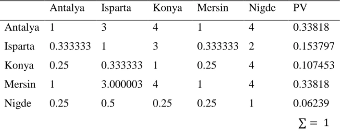
Table 5.7: Pairwise Comparison Matrix for Snow

Antalya 1 3 4 1 4 0.33818 Isparta 0.333333 1 3 0.333333 2 0.153797 Konya 0.25 0.333333 1 0.25 4 0.107453 Mersin 1 3.000003 4 1 4 0.33818 Nigde 0.25 0.5 0.25 0.25 1 0.06239 ∑ = 1 Inconsistency=0.08332

Table 5.8: Pairwise Comparison Matrix for Earthquake Risk

Antalya 1 3 2 2 3 0.351114 Isparta 0.333333 1 0.2 0.25 1 0.075117 Konya 0.5 5 1 1 3 0.251446 Mersin 0.5 4 1 1 3 0.23687 Nigde 0.333333 1 0.333333 0.333333 1 0.085453 ∑ = 1 Inconsistency=0.03426

(49)

39 Table 5.9: Pairwise Comparison Matrix for Population

Antalya 1 4 2 2 5 0.379254 Isparta 0.25 1 0.25 0.333333 2 0.082672 Konya 0.5 4 1 2 4 0.277722 Mersin 0.5 3.000003 0.5 1 5 0.205407 Nigde 0.2 0.5 0.25 0.2 1 0.054945 ∑ = 1 Inconsistency=0.03217

Table 5.10: Pairwise Comparison Matrix for Distance to CC

Antalya 1 0.5 0.333333 0.2 0.25 0.05912 Isparta 2 1 0.5 0.25 0.333333 0.092369 Konya 3.000003 2 1 0.25 0.25 0.129226 Mersin 5 4 4 1 2 0.423107 Nigde 4 3.000003 4 0.5 1 0.296178 ∑ = 1 Inconsistency=0.04321

Table 5.11: Pairwise Comparison Matrix for Distance to MR

Antalya 1 0.25 0.5 0.2 0.333333 0.062293 Isparta 4 1 2 0.5 2 0.245633 Konya 2 0.5 1 0.25 0.5 0.106735 Mersin 5 2 4 1 3 0.42225 Nigde 3.000003 0.5 2 0.333333 1 0.163089 ∑ = 1 Inconsistency=0.01583

(50)

40 To develop an overall priority matrix, the values of priority of each alternative, and the values of criterion priorities will be combined as shown in Table 5.12. The calculation for finding the overall priority of cities are shown below:

Overall priority of alternative 1 (Antalya)

(0.316145×0.401138)+(0.102704×0.308811)+(0.212612×0.384818)+(0.119354×0.1107

83)+(0.040096×0.055684)+(0.029644×0.33818)+(0.027554×0.351114)+(0.019388×0.3

79254)+(0.066252×0.05912)+(0.066252×0.062293)= 0.2909

The same calculation will be applied to find the overall priority for each alternative and the results are demonstrated in Table 5.13.

(51)

41 Table 5.12: Pairwise Matrix for all the Criteria.

C1 C2 C3 C4 C5 C6 C7 C8 C9 C10 PV C1 1 5.999988 3 4 8 7 7 9.000009 3 3 0.316145 C2 0.166667 1 0.2 0.5 4 5 5 5.999988 2 2 0.102704 C3 0.333333 5 1 2 7.000007 6 6 8 3 3 0.212612 C4 0.25 2 0.5 1 4 4 4 5 2 2 0.119354 C5 0.125 0.25 0.142857 0.25 1 2 2 4 0.5 0.5 0.040096 C6 0.142857 0.2 0.166667 0.25 0.5 1 1 2 0.5 0.5 0.029644 C7 0.142857 0.2 0.166667 0.25 0.5 1 1 2 0.333333 0.333333 0.027554 C8 0.111111 0.166667 0.125 0.2 0.25 0.5 0.5 1 0.333333 0.333333 0.019388 C9 0.333333 0.5 0.333333 0.5 2 2 3.000003 3.000003 1 1 0.066252 C 10 0.3333 33 0.5 0.3333 33 0.5 2 2 3.0000 03 3.0000 03 1 1 0.0662 52 Inconsistency=0.04229

(52)

42 Table 5.13: Overall Priority Matrix for the Cities.

Table 5.14: The Synthesized Priorities and Ranking the Cities Using AHP

Rank City Final Score

1 Mersin 0.241076

2 Antalya 0.212304

3 Isparta 0.183678

4 Konya 0.182332

5 Nigde 0.180609

Table 5.14 shows the final ranking of the AHP method and ranked the alternatives from the highest to lowest. Each score was obtained with respect to each alternative preference

C 1 (0.3 16145) C 2 (0.1 02704) C 3 (0.2 12612) C 4 (0.1 19354) C 5 (0.0 40096) C 6 (0.0 29644) C 7 (0.0 27554) C 8 (0.0 19388) C 9 (0.0 66252) C 10 (0.06 6252) Ove ra ll P V A1 0.401138 0.308811 0.384818 0.110783 0.055684 0.33818 0.351114 0.379254 0.05912 0.062293 0.2909 A2 0.091279 0.135554 0.115839 0.340218 0.164597 0.153797 0.075117 0.082672 0.092369 0.245633 0.14524 A3 0.093808 0.096882 0.071764 0.286765 0.348469 0.107453 0.251446 0.277722 0.129226 0.106735 0.13419 A4 0.307151 0.384239 0.365491 0.207435 0.125363 0.33818 0.23687 0.205407 0.423107 0.42225 0.3206 A5 0.106623 0.074515 0.062086 0.054799 0.305887 0.06239 0.085453 0.054945 0.296178 0.163089 0.10906

(53)

43 and the criteria selected in this study. Mersin scored the highest score with 0.241076 followed by Antalya with 0.212304, while Nigde ranked as the last alternative with 0.180609. The table demonstrates the potential in the field of solar power with the selected criteria for each alternative, and how they would perform.

5.2 ANP

After AHP, the second method applied in this study is ANP, the results obtained by this method using the program Super Decision, and the steps are explained below.

Similar to AHP, the following steps can be calculated either manually or automatically by the Super Decision software:

In this study, the application Super Decision was used to find the optimal alternative. ANP can be solved manually or using such applications. The usage of such applications is useful since it gives more accurate results with less time. The following procedure explains the ANP steps and how it can be done manually or automatically by the software: 1. Synthesizing the pair-wise comparison matrix is performed by dividing each element of the matrix by its column total. For example, the value 0.43796 in table 5.16 is obtained by dividing 1 from table 5.15 by 2.2833, the sum of the same column from table 5.15, (1+0.2+0.25+0.5+0.333333).

2. Eigen vector can be calculated by finding the row averages of the synthesized matrix. For example, the priority vector of Antalya is obtained by calculating the total of the first row (0.43796+0.37037+0.34783+0.52863+0.31579) and divide the result by the number of the alternatives, i.e. 5 to obtain the value. The priority vector for solar radiation (C1) demonstrated in table 5.16, is shown below.

[ 0.401138 0.091279 0.093808 0.307151 0.106623]