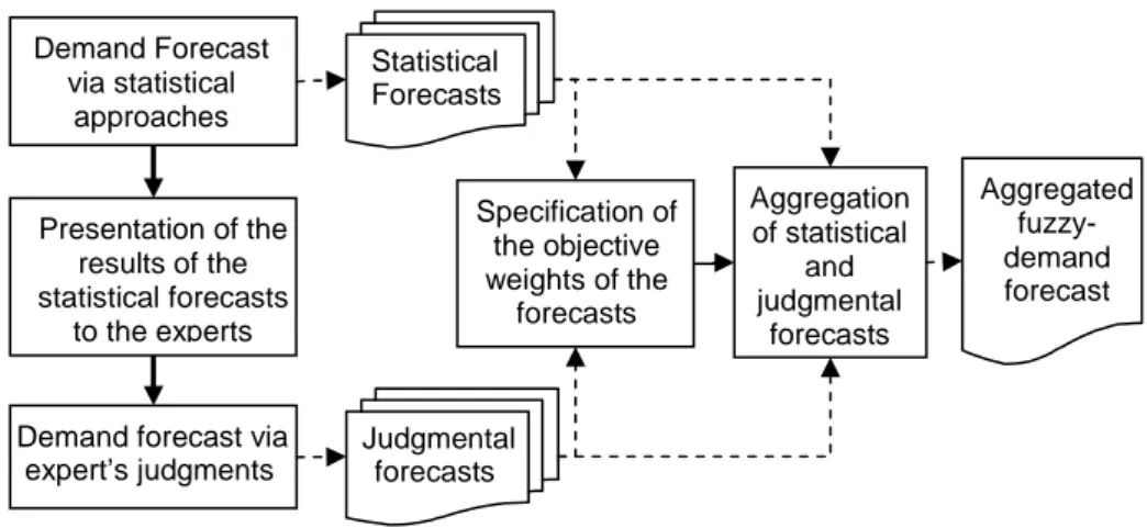
A demand forecasting methodology for fuzzy environments
Tam metin
Şekil

Benzer Belgeler
Açıklık sayısının deplasman profiline etkisini araştırmak için perdenin sistemin ortasında olduğu ve taban kesme kuvvetinin %50’sinini perde tarafından
Onerilen entropi fonksiyonuna dayalı uyarlanır karar t¨umles¸tirme yapısı (Entropy Functional Based Adaptive Deci- sion Fusion, EADF) yapısı bilgisayarlı g¨or¨uye dayalı
According to Padmanabhan’s proposal, the difference between the surface degrees of freedom and the bulk degrees of freedom in a region of space may result in the accelerated expansion
Bu bo˘gumların aynı a˘g ¨uzerinde bulundu˘gu fakat birbir- leri ile etkiles¸im ic¸inde olmadıkları durumlarda, her bo˘gum ic¸in ba˘gımsız olarak S¸ekil 1’de
In this work we study the necessary and sufficient conditions for a positive random variable whose expec- tation under the Wiener measure is one, to be represented as the
Beşinci hipotez; Organik Kimya dersinde portfolyo kullanımıyla destekli öğretim gören deney grubu ile klasik yöntemle öğretim gören kontrol grubunun öğretim
Cervical intradural disc hernia tion. Kataoka O, Nishibayashi Y, Sho T. Intradur<i! lumbar disc herniation. Report of three cases with a review of the literature. lntradural
Bu görüşm elerin ilk gü nünde, T ürkiye Büyük M illet Meclisi hüküm etinin tem silcileri, İstanbul hüküm etini tem silen gelen.. Sadrıâzam Tevfik Paşa
