Selçuk J. Appl. Math. Selçuk Journal of Vol. 6. No. 2. pp. 69-77, 2005 Applied Mathematics
Application of A New Mathematical Model for Estimating Maize Yield
Ufuk Karadavut1, A¸s¬r Genç2, Çetin Palta1, ¸Seref Aksoyak1
1 B.D. International Agricultural Research Institute, Po Box 125, Karatay - Konya,
Turkey;
2University of Selçuk, Department of Statistics, Selçuklu, Konya, Turkey.
e-mail:agenc@ selcuk.edu.tr
Received: November 25, 2005
Summary. This research was carried out International Agricultural Research Institute’s experimental areas in Konya province in the Central Anatolian Re-gion of Turkey. In the research, three corn cultivars (P 3394, DK 585 and NS 640) were tested in randomized complete block design with four replications. The interrelation between the productivity of Zea mays and the increasing of it’s generative organs during the phenological phase ‘tasseling-milky ripeness’, as far as the dependence of this relation on some factors in‡uencing crop grow, provide a basis for a quantity analysis left to this work. The potantial yield of the used hybrid was the only parametric index from the stock of the growth lim-iting factors, which take part in the analysis. Environmental factors, especially sum of e¤ective temperatures, precipitation and nitrogen supply, were strongly e¤ected yield formation. The interrelation between these factors gave us a real possibility to determine the function of the growth and yield.
Key words: Maize, Zea mays, Mathematical model, Yield formation
1. Introduction
Mathematical models of agricultural systems incorporate important known and/or hypothesized mechanizms (for example seasonality, interspesi…c competition, yield formation, harvesting) into a mathematical framework, for the purpose of tracking the spatial and temporal evaluation of variable of interest. Mathe-matical models are now frequently used to quantify complex biological systems [1, 2]. Thornley [3] has written at same lenght about mathematical models in plant physiology and emphasized that such models fall into two division as
mechanistic and emphirical model. Key…tz [4] has written a mathematical in-troduction to this …eld. Development of this area has occured mostly in the plant yield prediction. Models furthermore provide a unifying framework for thinking about the interplay between the various factors that govern a system [5]. This is an especially important advantage for complex studies as yield. Because of such characteristics, mathematical models are playing an increasing role in agriculture, biology and related …elds.
Yield formation is also very complex systems in maize growth. Yield are ef-fected by some genetic and environmental factors. Yield formation of maize is determinated by interaction between a variety of vegetative factors, as far as by the crop adaptation ability to unfavorable environmental condition. If a partic-ular factor is not in optimal quantity [6]. The crop adaptation ability decreases as regards to the other factors. An established fact is that the e¤ect of the limiting factor is manifested mainly during the reproductive period. Therefore the mathematical model of reproductive process give a real yield prognosis with the least deviation [7].
Mathematical models in estimating plant yields play such a large role. The functional approach to plant growth is a branch of mathematical modelling. A model is simply something constructed like something else and a mathematical model is a model constructed of mathematicals. So, a mathematical model expression, or a group of expressions that behaves in some way like a real system can be called a mathematical model of that system [8].
Alexieva et al. [7] developed a new mathematical model of the reproductive process of the zea mays in Bulgaria. This model is a mechanisitic model. The purpose of this paper is to illustrate the application of the mathematical model to estimate maize (Zea mays L.) yield grown in Turkey.
In section 2, we have explained plant material, its growing conditions and math-ematical presentation of growth function. In section 3, we have given results and discussion.
2. Meterial and Methods
2.1. Plant material and growing conditions
Field evaluation were conducted during 2003 and 2005 cropping seasons at the International Agricultural Research Institute’s experimental areas in Konya province in the Central Anatolian Region of Turkey (37o 52’ latitude, 32o 29’ longtitude and 1031 m high from sea level). The Soils of research area clay-loam texture, alkali (pH: 8.2), calcerously and slightly salt. Also, soils have medium organic matter (2.22 %), lime 7.4 % level, high potassium (1.812 ppm) and phosphorous (27.1 ppm).
In the research, three corn cultivars (P 3394, DK 585 and NS 640) were tested in randomized complete block design with four replications. Each year, the sowing the cultivars were sowned may at soil temperature 10 0C /10 cm soil depth. The size of each plot was 22.5 m2 with lenght-width of the row 5x4.5 m and distance between rows 0.75 m and 0.25 m between plants to give a plant population of 53 333 plants/ha.
At the planting, The nitrogen was applied to two equal splits; 75 kg/ha was applied in the form of urea with sowing, other 75 kg/ha 8 week after planting. Phosphor was applied in the form single superphosphate 50 kg/ha [9]. Weed control were practiced two times by hand when plants reached to 15-20 sand 35-40 cm.
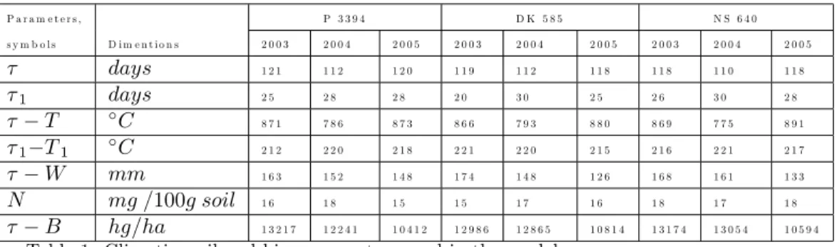
The vegetative biomass was determined in milky ripeness of crop, using 10 plants from each plot. The Quantity of and was determined in the phase ‘tasseling’ from a soil extract 1 M solution of KCL by means of calorimetric method [10]. The amount of precipitation and the sum of the e¤ective temperatures were measured and calculated for each phenologic phase (Table 1).
Relation between the growing function of the generative organs and crop yield is given by equation (8), where the known index is the potential crop yield of the hybrids used. As dependent variables some of the yield limitation factors were used [7]; P a r a m e t e r s , P 3 3 9 4 D K 5 8 5 N S 6 4 0 s y m b o l s D i m e n t i o n s 2 0 0 3 2 0 0 4 2 0 0 5 2 0 0 3 2 0 0 4 2 0 0 5 2 0 0 3 2 0 0 4 2 0 0 5 days 1 2 1 1 1 2 1 2 0 1 1 9 1 1 2 1 1 8 1 1 8 1 1 0 1 1 8 1 days 2 5 2 8 2 8 2 0 3 0 2 5 2 6 3 0 2 8 T C 8 7 1 7 8 6 8 7 3 8 6 6 7 9 3 8 8 0 8 6 9 7 7 5 8 9 1 1 T1 C 2 1 2 2 2 0 2 1 8 2 2 1 2 2 0 2 1 5 2 1 6 2 2 1 2 1 7 W mm 1 6 3 1 5 2 1 4 8 1 7 4 1 4 8 1 2 6 1 6 8 1 6 1 1 3 3 N mg =100g soil 1 6 1 8 1 5 1 5 1 7 1 6 1 8 1 7 1 8 B hg=ha 1 3 2 1 7 1 2 2 4 1 1 0 4 1 2 1 2 9 8 6 1 2 8 6 5 1 0 8 1 4 1 3 1 7 4 1 3 0 5 4 1 0 5 9 4
Table 1. Climatic, soil and bio- parameters used in the model
Where;
; Period germination-milky ripeness 1 ; Period tasseling-milky ripeness
T ; Sum of the e¤ective temperatures 1 T1 ; Sum of the e¤ective temperatures
W ; Amount of precipitation for the period
N ; Content of N N H4+ and N N O3 in tasseling B ; Dry biomass formulation for the period
W ; Amount of precipitation to the beginning of milky ripeness B ; Dry biomass formation during the period
The choise of variables was in conformity with the juncture that their measuring in the …eld was easier than other quantities connected with solar and water conditions [7].
2.2. Mathematical presentation of growth function during the reproductive period of Maize
We take that the crop yield y forming during the period germination to milky ripeness is proportional to the growth function during the reproductive period, i.e.:
(1) dy
d =
daj d
The function aj depend on the potential for the hybrid yield -a, as well as the complex interaction of j-parameters- B; N; 1; T; T1; W: On the account of that the equation (1) could be presented as a characteristic congruence from two indexes T and N and it is expressed by particular derivatives i.e.:
(2) daj d = @ @ aj T dT d + @ @ aj N dN d
According to superposition the general integral of the equation (2) is a linear relation of particular integrals. At a given value of the argument a and rvalues for T and 1, got from observations, the …rst term of (2) could be presented by function: @ @ aj T 1 d aj=a:dT = f1(a; 1; T ):dT where f1(a; 1; T ) = a T: 1
From the integration of the …rst term of (2) a particular integral will be esti-mated: (3) I1= a T: 1 T Z 0 dT = a T 1 T1
After transformation of the second term of (2) the same equation could be expressed as: (4) @ @ aj N dN d aj=B = @ @ B W 1 @ @ W N dN
Expression in the brackets in (4) is presented by the function, in which argu-ments are B; W; : Their numerical values are obtained from …eld measureargu-ments, so that this expression is presented as follows:
(5) @ @ B W 1 = f2(B; W; ) = B W:
The quantity of the N N H4+ and N N O3 in soil linearly depend on the volumetric moisture W0, so that the the derivative in the right part of (4) is converted to: (6) @ @ W NdN = dN N @ @ W W0W0
From (5) and (6) the following expression for the second particular integral in (2) is generated: (7) I2= B W: Z Z D dN N @ @ W W0W0= B W: N Z 0 dN N W k Z 0 f3(W0)dW
The soil of integral in (7) is by means of the parameter W k (the mean critical soil moisture for dissolving and suction of the mineral salts from the soil solution). The optimal value of W k is 0.75 of …eld capasity [11]. The general integral in (2) will be: aj = a T: 1 T1 0:75W k B W: ln N
and the equation for yield prediction takes on the following expression:
(8) y = a
T: 1
T1 0:75W k B
W: ln N :
We used the mathematical model to estimate maiz yield following expression;
y = a
T: 1
T1 0:75 B
W: ln N :
and we also used statistical model to estimate maiz yield following expression;
Y = 0+ 1X1+ 2X2+ 3X3+ 4X4+ 5X5+ 6X6+ 7X7+ 8X8+ 9X9+ 10X10+"
where; o; 1; 2; 3; 4; 5; 6; 7; 8; 9; 110ve " are plant height, ear height, ear length, ear dimension, ear weight, number of seed/ear, weight of seed/ear, number of ear/plant, 100 seed weight, number of days until ‡owering and error respectively.
3. Results and Discussions
Zea mays plants show no change in dry weight for the …rst days of the growth or so. Then it actually losses weight after about end of ripening period. There has been considerable di¤erentiation of leaf tissue in the young seedling (at the expense of total dry weight). Climatic and environmental conditions e¤ected strongly on yield formation of cultivar.
A high biomass formation and high grain yield respectively were observed in 2003 when combination between T and W was in optimum. The lowest quantity biomass and lowest yield were registered in 2005. P 3394 cultivars gave a highest biomass, NS 640 also gave the lowest biomass all years. A comperative valuation between the real and estimated by model yield was done (Table 2).
The yield estimated by means of the model works with a maximum relative error
8:38%(P3394), minimum relative error 0:31% (DK 585) and for all cultivars relative error is 3:30% in mathematical estimation. But in ststistical esti-mation, maximum relative error is 2:50% (NS 640), minimum relative error 0:40% (P 3394) and for all cultivar relative error is 1:21%. This give us reason to use As a result, this model is used succesively for yield prediction zea mays cultivar that is grown in Turkey during whole period.
P a r a m e t e r s , P 3 3 9 4 D K 5 8 5 N S 6 4 0 s y m b o l s D i m e n t i o n s 2 0 0 3 2 0 0 4 2 0 0 5 2 0 0 3 2 0 0 4 2 0 0 5 2 0 0 3 2 0 0 4 2 0 0 5 y K g / h a 1 4 0 1 0 1 5 9 2 1 1 4 4 7 4 1 5 0 7 5 1 7 1 7 3 1 7 5 5 8 1 4 4 8 1 1 6 6 7 0 1 5 7 7 5 y K g / h a 1 5 1 7 5 1 5 0 6 2 1 4 9 1 2 1 4 6 0 7 1 6 8 6 2 1 6 9 5 5 1 3 8 6 2 1 7 6 3 8 1 6 0 2 0 SX K g / h a 4 5 8 8 6 2 6 5 4 7 8 9 9 2 4 8 8 4 1 0 2 1 6 8 4 5 4 2 C o e f . o f V a r % 3 . 0 2 5 . 7 2 4 . 3 9 5 . 4 0 5 . 4 8 5 . 2 1 7 . 3 7 3 . 8 8 3 . 3 8 " % 8 . 3 2 5 . 3 9 3 . 0 6 - 0 . 3 1 - 1 . 8 1 3 . 4 3 4 . 2 7 5 . 8 1 1 . 5 5 y K g / h a 1 3 9 5 4 1 5 8 2 1 1 4 7 2 3 1 4 9 5 2 1 6 9 6 2 1 7 2 1 1 1 4 1 2 8 1 6 8 1 0 1 5 6 4 1 SX K g / h a 2 9 8 3 1 5 2 9 6 2 1 5 4 1 2 3 6 8 7 5 1 5 2 1 2 2 9 R2 - 0 . 9 6 0 . 9 4 0 . 8 9 0 . 9 4 0 . 9 1 0 . 8 7 0 . 8 5 0 . 9 3 0 . 9 3 C o e f . o f V a r % 2 . 1 4 1 . 9 9 2 . 0 1 1 . 4 4 2 . 4 3 2 . 1 4 5 . 3 2 3 . 0 9 1 . 6 4 " % 0 . 4 0 0 . 6 3 1 . 7 2 0 . 7 8 1 . 2 3 1 . 9 8 2 . 5 0 0 . 8 4 0 . 8 5
Table 2. Valuation of the model precition
y ;Real Yield
y ;Estimated Yield (With mathematical model) y ;Estimated Yield (With statistical model) " = (y y)=y;Relative error
According to cultivars observed, explained with mathematical and statistical models and estimated for 2006 year yields are shown in Figure 1, 2 and 3. When these results are investigated, see that the statical methods are more explenatary than the mathematical models at all cultivars. Although the mathematical model presented here is simple to be useful in the …eld, it has’t explained maize yield . The validation of quantitative biological models is not simple problem. Methods must account for the multiplicity of error in both the observed and the predicted values. Models can be parameterised with …eld data, and results from simulations can be used to test hypoteses and make predictions. However, such models can be computationally very intensive. Moreover, it is often di¢ cult to interpret the results. Further collaboration between mthematical- statistical
models and plant growth experts may increase the applications of this models in plant growth. In much the same way that mathematical and statistical models have been applied to other plants.
The yield estimated by means of the model works with a maximum relative error
% (P3394) and minimum relative error % (DK 585). For all cultivar relative error is %. This give us reason to use As a results, this model is used succesively for yield prediction zea mays cultivar that is grown in Turkey during whole period
Observed, explained with mathematical and statistical models in 2003 (1),2004 (2), 2005 (3) and their estimations (4) in 2006 for P 3394 cultivar
Observed, explained with mathematical and statistical models in 2003 (1),2004 (2),
2005 (3) and their estimations (4) in 2006 for DK 585 cultivar
Observed, explained with mathematical and statistical models in 2003 (1), 2004 (2), 2005 (3) and their estimations (4) in 2006 for NS 640 cultivar
References
Butterworth and co., London.
2. Murray J. D. (1993): Mathematical Biology. Springer, Berlin.
3. Thornley J. H. M. (1976): Mathematical Models in Plant Physiology. Quantitative Approach to Problems in Plant and Crop Physiology, Academic Press, London. 4. Key…tz N. (1968): Introduction to The Mathematics of Population. Addison-Wasley, Reading. Mass.
5. Bauch C. T. and Anand M. (2004): The Role of Mathematical Models in Ecological Restoration and Management. International Journal of Ecology and Environmental Sciences 30 : 117-122. International Scienti…k Publications, New Delhi.
6. Schelford V. (1964): The Ecology North America. Univer of Ill¬noise Press. 7. Alexieva S. G., Stoimenova I. A. and Mikova A. G. (1997): A Dynamic Modelling of The Reproductive Process of Zea Mayze. First European for Information Tecnology in Agriculture, Cophenagen, 15-18 June 1997.
8. Hunt R. (1982): Plant Growth Curves. The Functional Approach to Plant Growth Analysis.
9. Sade B. (2002): M¬s¬r Tar¬m¬. Konya Ticaret Borsas¬. Yay¬n numaras¬ 1, ·Ikinci
Bask¬. Konya.
10. Jagodina B. A. (1987): Practicum for Agrochemistry. Agropromizad. Moskova, pp. 276-280.
11. Tomov N. Jordanov (1989): Mayze in Bulgarien. Zemizat, pp. 230-251. So…a-Bulgarian.