Selçuk J. Appl. Math. Selçuk Journal of Vol. 10. No.1. pp. 45-61, 2009 Applied Mathematics
Homotopy Analysis Solution of Three Dimensional Diffusion Equa-tions
G. Domairry1, M. Ghanbarpour, F. Ghanbarpour
1Department of Mechanical Engineering, Babol University of Technology , P.O. Box
484, Babol, Iran
e-mail: am irganga111@ yahoo.com
Received: April 9, 2008
Summary. In this paper, the Homotopy Analysis Method (HAM) is employed to find a suitable solution for parabolic equations. This method is a strong and easy—to—use analytic tool for investigating linear and nonlinear problems, which do not need small parameters. Homotopy analysis method contains the auxiliary parameter ~, which provides us with a simple way to adjust and control the convergence region of solution series.
By suitable choice of the auxiliary parameter ~, we can obtain reasonable so-lutions for large modulus. In this study, we compare obtained results through (HAM) with the exact solutions. This type of equations governs on numerous scientific and engineering experimentations.
Keywords: Homotopy Analysis Method (HAM), nonlinear parabolic equa-tions.
2000 Mathematics Subject Classification: 35N05, 35B20. 1. Introduction
Partial differential equations which arise in real-world physical problems are often too complicated to be solved exactly. And even if an exact solution is obtainable, the required calculations may be too complicated to be practical, or it might be difficult to interpret the outcome. Recently, some promising approximate analytical solutions are proposed, such as exp-function method [1-2], Adomian’s decomposition method [3-4], variational iteration method [5-6] , homotopy-perturbation method [7-8] and homotopy analysis method(HAM) [9,10]. Most scientists believe that the combination of numerical and semi-exact analytical methods can also end with useful results. Homotopy Analysis Method (HAM) is one of the well-known methods to solve the linear and nonlinear equations which was expressed by Liao [11-14] and studied by a large number of
researchers such as G. Domairry [9] and many of them such as Abbasbandy [15] and T.Hayat [16] applied HAM in heat transfer. Liao in [14] proved that ADM is a special case of the HAM and Dr.Allan applied this kind of relationship in [17].
In this study, the general parabolic equation in the form of:
(1a) = (−→ )+ (−→ )+ (−→ )+ (−→ )
where,
(1b) = + +
is to be solved.
The Liao’s Homotopy analysis method (HAM) 2.1. The basic idea [11-14]
Consider the following differential equation
(2) [ ( )] = 0
where, is a nonlinear operator, denotes the independent variable, ( ) is the unknown function. For simplicity, we ignore all boundary or initial conditions, which can be treated in the similar way. By means of generalizing the traditional homotopy method, Liao [14] constructed the so-called zero-order deformation equation
(3) (1 − ) [(; ) − 0( )] = ~() [( ; )]
where ∈ [0 1] is the embedding parameter, ~ 6= 0 is a nonzero auxiliary parameter, ( ) 6= 0 is an auxiliary function, is an auxiliary linear operator, 0( ) is an initial guess of ( ) and ( ; ) is an unknown function. It is
important that one has a great freedom to choose auxiliary unknowns in HAM. Obviously, when = 0 and = 1 it holds
( ; 0) = 0( ) ( ; 1) = ( )
respectively. Thus, as increases from 0 to 1, the solution ( ; ) varies from the initial guess, 0( ) to the solution ( ). Expanding ( ; ) in Taylor series
with respect to, we have
(4) ( ; ) = 0( ) +
+∞
X
=1
where, (5) ( ) = 1 ! ( ; ) |=0
If the auxiliary linear operator, the initial guess, the auxiliary parameter ~, and the auxiliary function are quite properly chosen, the series (4) converges at = 1 then we have (6) ( ) = 0( ) + +∞ X =1 ( )
which must be one of the solutions of the original nonlinear equation as proved by Liao [14]. As ~ = −1 and ( ) = 1 Eq. (3) becomes
(1 − )[(; ) − 0( )] + [( ; )] = 0
This is mostly used in the HPM, whereas the solution can be obtained directly without using Taylor series [11, 12].
According to the Eq. (5), the governing equation can be deduced from the zero-order deformation Eq. (3). Defined the vector
= {0( ) 1( ) ( )}
Differentiating Eq. (3) for times with respect to the embedding parameter , and then setting = 0 and finally dividing them by !, we have the so-called mth-order deformation equation
(7) [( ) − −1( )] = ~()(−1) where, (8) (−1) = 1 ( − 1)! −1 [( ; )] −1 ¯ ¯ ¯ ¯=0 and = ½ 0 ≤ 1 1 1
It should be emphasized that ( ) for ≥ 1 is governed by the linear Eq. (7)
with the linear boundary conditions coming from the original problem, which can be easily solved by using symbolic computation software such as Maple and Mathematica.
2.2. Application
In order to assess the accuracy of HAM for solving linear or nonlinear parabolic equations with variable physical parameters and to compare it with exact, we will consider the four following examples.
2.2.1. Example 1. Consider Eq. (1a), with the following assumptions to make it more specific:
(9) = 1 ( ) = ( ) = 0 ( ) = ( ) = 1 Therefore
(10) = +
With the new initial condition
(11) ( 0) = (+)
We choose the initial guesses and auxiliary linear operator in the following form:
(12) 0( ) = (+)
(13) (( )) = ( )
We construct the following problems:
Zeroth —order deformation problems
(14) (1 − ) [( ; ) − 0( )] = ~ [( ; )] (15) [( )] = ( ) − ( 2( ) 2 ) − ( 2( ) 2 ) For = 0and = 1 we have (16) ( ; 0) = 0( ) ( ; 1) = ( )
When increases from 0 to 1 then ( ; ) vary from 0( )to ( ) .
( ; ) = 0( ) + ∞ X =1 ( ) where (17) ( ) = 1 ! (( ; )) Then we have (18) ( ) = 0( ) + ∞ X =1 ( )
mth —order deformation problems
(19) [( ) − −1( )] = ~( ) (20) ( 0) = 0 (21) = (−1)− (−1)− (−1) (22) = ½ 0 ≤ 1 1 1
The following terms are solutions for three term of the solution.
(23) 1( ) = −2~(+) (24) 2( ) = 2= −2~+− 2~2++ 2~22+ (25) 3( ) = −2+ µ ~ + 2~2 + ~3 − 2~32− 2~22+2 3~ 33 
The solution 4( ) was too long to be mentioned here, therefore, it is shown
2.2.2. Example 2. Consider Eq. (1a), with the following assumptions to make it more specific:
(26) = 1 = = 0 (−→ ) = 1 (−→ ) = 1 Therefore
(27) = +
with the initial condition
(28) ( 0) =
We choose the initial guesses and auxiliary linear operator in the following form
(29) 0( ) =
(30) (( )) = ( )
We construct the following problems:
Zeroth —order deformation problems
(31) (1 − ) [( ; ) − 0( )] = ~ [( ; )] (32) [( )] = ( ) − ( 2( ) 2 ) − ( 2( ) 2 )
For = 0and = 1 we have
(33) ( ; 0) = 0( ) ( ; 1) = ( )
When increases from 0 to 1 then ( ; ) vary from 0( )to ( ) .
Due to Taylor series with respect to , we have ( ; ) = 0( ) + ∞ X =1 ( ) where
(34) ( ) = 1 ! (( ; )) Then we have (35) ( ) = 0( ) + ∞ X =1 ( )
mth —order deformation problems
(36) [( ) − −1( )] = ~( ) (37) ( 0) = 0 (38) = (−1)− (−1)− (−1) (39) = ½ 0 ≤ 1 1 1
The following terms are solutions for three term of the solution.
(40) 1( ) = −~ (41) 2( ) = −~ − ~2 + 1 2~ 22 (42) 3( ) = −~ − ~2 +12~22+ ~(−~ − ~2 + 12~22) − ~(−12~2− 1 2~22+ 1 6~23)
The solution 4( ) was too long to be mentioned here, therefore, it is shown
graphically.
2.2.3. Example 3. Consider Eq. (1a), with the following assumptions to make it more specific:
Therefore the following equation is derived to be solved as the second example:
(44) = + +
with the new initial condition of
(45) 0( ) = (1 − )(+)
Similar to previous example, we choose the initial guesses and auxiliary linear operator in the following form:
(46) 0( ) = (1 − )(+)
(47) (( )) = ( ) We construct the following problems:
Zeroth —order deformation problems
(48) (1 − ) [( ; ) − 0( )] = ~ [( ; )] (49) [( )] = ( ) −( 2( ) 2 )−( 2( ) 2 )−( 2( ) 2 )
For = 0and = 1 we have
(50) ( ; 0) = 0( ) ( ; 1) = ( )
When increases from 0 to 1 then ( ; ) vary from 0( ) to
( ) . Due to Taylor series with respect to , we have ( ; ) = 0( ) + ∞ X =1 ( ) where, (51) ( ) = 1 ! (( ; )) Then we have
(52) ( ) = 0( ) + ∞
X
=1
( )
mth —order deformation problems
(53) [( ) − −1( )] = ~( ) (54) ( 0) = 0 (55) = (−1)− (−1)− (−1)− (−1) (56) = ½ 0 ≤ 1 1 1
The following terms are solutions for three term of the solution.
(57) 1( ) = −2~(1 − )(+) (58) 2( ) = −2~(1 − )(+) − 2~2(1 − )(+) + 2~2(1 − )(+)2 (59) 3( ) = −2~(1 − )(+) − 2~2(1 − )(+) + 2~2(1 − )(+)2 +~(−2~(1 − )(+) − 2~2(1 − )(+) + 2~2(1 − )(+)2) −2~(−~(1 − )(+)2− ~2(1 − )(+)2+2 3~2(1 − )(+)3)
The solution 4( ) was too long to be mentioned here, therefore, it is
shown graphically.
2.2.4. Example 4. Consider Eq. (1a), with the following assumptions to make it more specific:
(60) = 1 = 0 (−→ ) = 1 (−→ ) = 1
(61) = +
with the new initial condition of
(62) ( 0) = (1 − )
We choose the initial guesses and auxiliary linear operator in the following form:
(63) 0( ) = (1 − )
(64) (( )) = ( )
We construct the following problems:
Zeroth —order deformation problems
(65) (1 − ) [( ; ) − 0( )] = ~ [( ; )] (66) [( )] = (( ) ) − ( 2( ) 2 ) − ( 2( ) 2 )
For = 0and = 1 we have
(67) ( ; 0) = 0( ) ( ; 1) = ( )
When increases from 0 to 1 then ( ; ) vary from 0( )to ( ) .
Due to Tailors’ series with respect to , we have ( ; ) = 0( ) + ∞ X =1 ( ) where, (68) ( ) = 1 ! (( ; )) Then we have (69) ( ) = 0( ) + ∞ X =1 ( )
mth —order deformation problems (70) [( ) − −1( )] = ~( ) (71) ( 0) = 0 (72) = (−1)− (−1)− (−1)− (−1) (73) = ½ 0 ≤ 1 1 1
The following terms are solutions for three term of the solution.
(74) 1( ) = −~(1 − ) (75) 2( ) = −~(1 − ) − ~2(1 − ) + 1 2~ 2 (1 − )2 (76) 3( ) = −~(1 − ) − ~2(1 − ) + 12~2(1 − )2 +~(−~(1 − ) − ~2(1 − ) +12~2(1 − )2) −~(−12~(1 − ) 2 −12~ 2 (1 − )2+16~2(1 − )3)
Like previous case, the solution 4( ) was too long to be mentioned here,
therefore, it is shown graphically.
3. Convergence of the HAM solution.
As pointed out by Liao, the convergence and rate of approximation for the HAM solution strongly depends on the values of auxiliary parameters ~. Figs (1—4) clearly depict that the ranges, for admissible values of ~ for example 1 is −095 ~ −11 , for example 2, is −15 ~ −08, for example 3, is −095 ~ −11 and for example 4, is −095 ~ −11 .Our calculations clearly indicate that series converge for whole region of variable parameters when~ = −1.
Fig.1. Curve for = 1, = 1, = 01 by 5th-order approximation of solution
for example 1
Fig.2. Curve for = 1 = 1 = 1 by 5th-order approximation of solution
for example 2
Fig.3. Curve for = 1, = 01, = 1 = 01 by 5th-order approximation of
solution for example 3
Fig.4. Curve for = 1, = 01, = 01 by 5th-order approximation of solution
for example 4
4. Comparing the results with the exact solutions.
The comparison of the result of the HAM and exact solutions are given in following figures.
Fig.5. plot of HAM result of the ( ) at = −1, = 1 for example 1
Fig.6. plot of exact solution of the ( ) at = 1 for example 1
Fig.7. plot of HAM result of the ( ) at = −1, = 1 for example 2
Fig.8. plot of exact solution of the ( ) at = 1 for example 2
Fig.9. plot of HAM result of the ( ) at = −1, = 01, = 1
for example 3
Fig.10. plot of exact solution of the ( ) at = 01, = 1 for
example 3
Fig.11. plot of HAM result of the ( ) at = −1, = 01 for
example 4
Fig.12. plot of exact solution of the ( ) at = 01 for
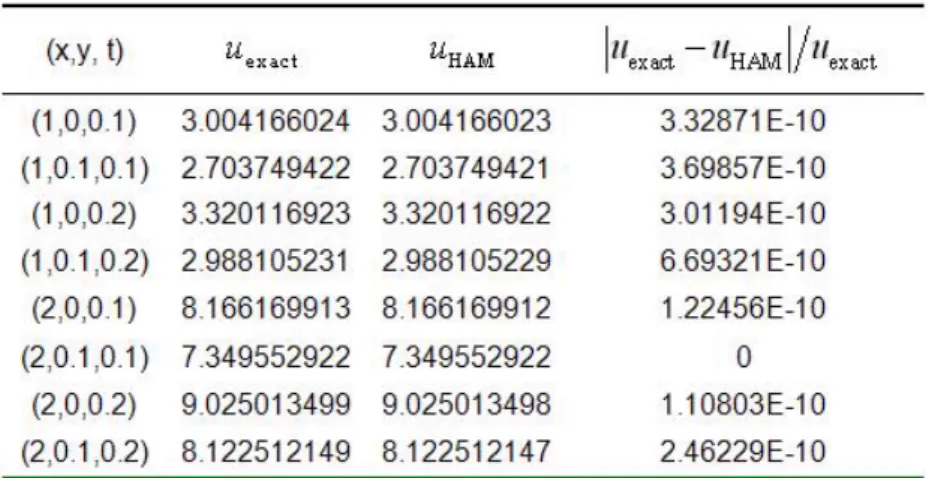
Table 1. The HAM results for example 1 for the first five approximations in comparison with theanalytical solutions
Table 2. The HAM results for example 2 for the first five approximations in comparison with the analytical solutions.
Table 3. The HAM results for example 3 for the first five approximations in comparison with the analytical solutions.
Table 4. The HAM results for example 4 for the first five approximations in comparison with the analytical solutions.
5. The comparison of the methods and conclusions
Results clearly show that Homotopy Analysis Method applied to the equations was capable of solving them with successive rapidly convergent approximations without any restrictive assumptions or transformations causing changes in the physical properties of the problem. Also adding up the number of iterations leads to the explicit solution for the problem. In HAM we can choose ~ in an appropriate way. The results show us the validity and great potential of the HAM for linear and nonlinear parabolic equations
References
1. S. Zhang. Exp-function method exactly solving a KdV equation with forcing term. Appl Math Comput, 2008, 197, 128-134.
2. S.A. El-Wakil, M.A. Abdou and A. Hendi. New periodic wave solutions via Exp-function method Phys. Lett. A,2008 372, 830-840.
3. O. Abdulaziz, N.F.M. Noor, I. Hashim and M.S.M. Noorani, Further accuracy tests on Adomian decomposition method for chaotic systems, Chaos, Solitons & Fractals 2008, 36, 1405-1411.
4. R. Memarbashi, Numerical solution of the Laplace equation in annulus by Adomian decomposition method, Chaos, Solitons & Fractals, 2008, 36, 138-143.
5. D.D. Ganji, G.A. Afrouzi and R.A. Talarposhti, Application of He’s variational it-eration method for solving the reaction—diffusion equation with ecological parameters, Comp & Math Appl, 2007, 54, 1010-1017.
6. D.D. Ganji, Hafez Tari and M. Bakhshi Jooybari ,Variational iteration method and homotopy perturbation method for nonlinear evolution equations, Comp& Maths Appl,2007,54, 1018-1027.
7. D.D. Ganji, A. Sadighi, Application of He’s Homotopy-perturbation Method to Nonlinear Coupled Systems of Reaction-diffusion Equations, Int.j.nonl science and numl simul, 2006, 7, 413-420.
8. A.M. Siddiqui, R. Mahmood, Q.K. Ghori, Homotopy-perturbation method for thin film flow of a fourth grade fluid down a vertical cylinder, Phys. Lett. A, 2006, 352, 404-410.
9. G. Domairry and N. Nadim, Assessment of homotopy analysis method and ho-motopy perturbation method in non-linear heat transfer equation, Int Commun Heat Mass Trans 2008, 35, 93-102.
10. Z. Ziabakhsh and G. Domairry, Solution of the Laminar Viscous Flow in a Semi-porous Channel in the Presence of a Uniform Magnetic Field by using the Homotopy Analysis Method, Commun nonlinear Science and Numl Simul, 2009, 14 (4):1284—1294. 11. S.J. Liao, The proposed homotopy analysis technique for the solution of nonlinear problems. Ph.D. thesis, Shanghai Jiao Tong University; 1992.
12. S.J. Liao, An approximate solution technique not depending on small parameters: a special example. Int J Non-Linear Mech 1995;303:371—380.
13. S.J. Liao, On the homotopy analysis method for nonlinear problems, Appl. Math. Comput. 147 (2) (2004) 499—513.
14. Liao SJ. Beyond perturbation: introduction to the homotopy analysis method. Boca Raton: Chapman & Hall, CRC Press; 2003.
15. S. Abbasbandy, The application of homotopy analysis method to nonlinear equa-tions arising in heat transfer, Phys. Lett. A, 360(2006)109-113.
16. T. Hayat and M.Sajid, On analytic solution for thin film flow of a forth grade fluid down a vertical cylinder, Physics Letter A, 361(2007)361-322.
17. F.M. Allan, Derivation of Adomian decomposition method using the homotopy analysis method, Applied Mathematics and Computation, 190(2007)6-14.