Application of dither and observer based state feedback in the control of chaotic systems

/ .... ·' <? Ι Ψ Ζ - S • C h S u j ^ a і з а б β ц f. ^ ''^ · ?л.®. -ÎÇ’ .?· fr* î *5^ Ί% ■<■., ν· ;^. .İ Ä ;ч ;,ί> ·λ·. :Г. η -j

-Λύ Τ L V b ñ l İİJ^l b S b ' l ü b l t î:: f

APPLICATION OF DITHER AND OBSERVER

BASED STATE FEEDBACK IN THE CONTROL. OF

CHAOTIC SYSTEMS

A THESIS

SUBMITTED TO THE DEPARTMENT OF ELECTRICAL AND ELECTRONICS ENGINEERING

AND THE INSTITUTE OF ENGINEERING AND SCIENCES OF BILKENT UNIVERSITY

IN PARTIAL FULFILLMENT OF THE REQUIREMENTS FOR THE DEGREE OF

MASTER OF SCIENCE

By

Umut Ersoy

August 1996

tarafinJiui bcfiflanmifiif.

Q. ■ІЧХ5 • C 4 S ■U43

■1936

ß. i >14 í> 5 я

I certify that I have I’ead this thesis and that in my opinion it is fully adequate, in scope and in quality, as a thesis lor the degree of Master of Science.

Assoc. Prof. Dr. Omer Morgiil (Supervisor)

1 certify that I have read this thesis and that in my opinion it is fully adequate, in scope and in quality, as a thesis for the degree of Master of Science.

A 'I

Prof. Dr. Erol Sezer

I certify that I have read this thesis and that in my opinion it is fully adequate, in scope and in quality, as a thesis for the degree of Master of Science.

Prof. Dr. Bülent Özgüler

Approved for the Institute of Engineering and Sciences:

Prof. Dr. Mehrnet l^ajxiy

ABSTRACT

APPLICATION OF DITHER AND OBSERVER BASED

STATE FEEDBACK IN THE CONTROL OF CHAOTIC

SYSTEMS

Umiit Ersoy

M.S. in Electrical and Electronics Engineering

Supervisor: Assoc. Prof. Dr. Orner Morgiil

August 1996

In the first part of this thesis, the application of dither for controlling chaotic systems is presented. Dither is a high frequency periodic signal that has been excunined in the literature before, for changing nonlinear systems effectively. The presented technique is based on a conjecture proposed by Genesio and Tesi and is mainly cipplicable to systems in Lur’e form.

In the second part, the application of state feedback is presented. Unknown states of the system are constructed by using nonlinear full-state observers. The control strategy is mainly based on the mentioned conjecture and also on bifurcation diagriuns.

Keywords : Chciotic dynamics, describing function analysis, dither, ob­ servers, state feedback, bifurcation diagrams.

ÖZET

KIPIRTILANDIRMANIN VE GÖZLEYİCİ TABANLI

DURUM GERİBESLEMESİNİN KAOTİK SİSTEMLERİN

KONTROLÜNDE UYGULAMASI

Umut Ersoy

Elektrik ve Elektronik Mühendisliği Bölümü Yüksek Lisiuıs

Tez Yöneticisi: Doç. Dr. Ömer Morgül

Ağustos 1996

Bu tezin ilk bölümünde kıpırtının (dither) kaotik sistemlerin kontrolünde uygulanması anlatılmıştır. Kıpırtı (dither), bundan önce literatürde, doğrusal olmayan sistemlerin etkili bir biçimde değiştirilmesi konusunda incelenmiş, yüksek frekanslı periyodik bir sinycüdir. Burada anlatılan teknik, başlıca Lur’e formdaki sistemlere uygulanabilir ve Genesio ve Tesi tarafından önesürülmüş bir varsayıma dayanmaktadır.

İkinci bölümde, durum geribeslemesinin kaotik sistemlerin kontrolünde uygulanması anlatılmıştır. Sistemin bilinmeyen durumları, doğrusal olmayan türn-durum gözleyicileri ile elde edilmiş, kontrol stratejisi ise yine hem bahsi geçen varsayıma, hem de çatallanma (bifurcation) şemalarına dayandırılmıştır.

A.ncıhtcır Kelimeler Kaotik ha.reketler, tanımlayıcı foıı.sıyon analizi, kıpııtı (dither), gözleyiciler, durum geribeslemesi, çatallanma şemaları.

ACKNOWLEDGEMENT

I would like to express my gratitude to Dr. Ömer Morgiil lor his super­ vision, guidance, suggestions and invaluable encouragement throughout the development of this thesis.

I would also like to thank to Dr. Erol Sezer and Dr. Bülent Özgüler tor reading and commenting on the thesis.

TABLE OF C O N TE N TS

1 Introduction 1

1.1 Chaos P henom enon... 1

1.2 Controlling C h a os... 3

2 The Conjecture of Genesio and Tesi 5

2.1 Prediction of Limit C y c l e s ... 6

2.2 Equilibrium P o i n t s ... 8

2.3 Filtering Effect 9

2.4 Interaction... 9

3 Dither Control of Chaotic Systems 11

3.1 D i t h e r ...

3.2 Application of Dither on the Control of Chaotic Systems . . . . 15

3.2.1 Control Based on Equilibrium Point Elim ination... 16

3.2.2 Control Based on Interaction 1”

3.2.3 Control Based on Bifurcation Diagrilrns... 20

3.3 Application Examples 21 3.3.1 Cliua’s C ircu it... 21

3.3.2 Relay S y s t e m ... 24

3.3.3 System with a Scpiare N o n lin e a rity ... 27

3.3.4 System with a Cubic N onlinearity... 29

3.3..5 Duffing O scillator... 31

4 Observer Based Feedback Control of Chaotic Systems 33 4.1 O b s e r v e r s ... 33

4.1.1 Linear O b s e r v e r s ... 34

4.2 Observer Based State Feedback Control of Chciotic Systems 36 4.2.1 Feedback Control Based on In te ra ctio n ... 37

4.2.2 Feedback Control Based on Bifurcation Diagrams . . . . 38

4.3 Application Examples 39 4.3.1 Chua’s C ircuit... 39

4.3.2 Relay S y s t e m ... dO

4.3.3 Duffing Oscillcitor... l ‘-l

4.3.4 Forced Van der Pol O s c illa t o r ... d3

5 Conclusion 46

LIST OF FIGURES

2.1 General configuration of a system in Lur’e f o r m ... 6

3.1 Application of dither to a system in Lur'e form 11

3.2 Compensating nonlinear fe e d b a c k ... 18

3.3 Chua’s c i r c u i t ... 21

3.4 Chaotic attractors of Chua’s c i r c u i t ... 23

3.5 Chua’s nonlinearity before and after the application of dither 23

3.6 Actual and predicted limit cycles of Chua’s circuit after the ap­

plication of dither 24

3.7 Chaos in the relay system 25

3.8 Nonlinearity of the relay system before and after the a.pplication of d i t h e r ... ‘46

3.9 Actual and predicted limit cycles of the relay system after the

application of dither 26

3.10 Chaos in the system with square nonlinearity 28

3.11 Actual and predicted limit cycles of the systfem with sc[uare non­

linearity after the cipplication of dither 28

3.12 Chaotic behavior for the system with cubic nonlinearity. 30

3.13 Limit cycles for the system with cubic non. after the application

of dither. 30

3.14 Chaotic behavior of the Duffing oscillator 32

3.L5 Limit cycle for the Duffing oscillator after the application of

dither 32

4.1 Feedbcick based on observer configuration

4.2 Limit cycle of the Chua’s circuit after feedback is applied

4.3 Limit cycle of the relay system after feedback is applied

4.4 Limit cycle of the Duffing oscillator

4..5 Chaos of the Duffing oscillator after feedback is applied

4.6 Chaotic behavior of the Van der Pol oscillator

37 40 41 42 43 44

4.7 Limit cycle of the Vein der Pol oscillator after feedback is applied 4.5

Chapter 1

Introduction

Chaos is one of the most popular subjects in many different fields of science in the last few decades. With the appearance of high speed, high capacity computers, the simulation and analysis of nonlinear dynamical systems which were very difficult and in some cases impossible before, have become possible in recent years. This powerful tool has forced an extensive research on less un­ derstood nonlinear dynamics resulting in a complex and exciting phenomenon, namely chaos.

1.1

Chaos Phenomenon

Although it has been observed in many dynamical systems, there is not a uni­ versally accepted definition lor the term chaos. A generally accepted inloimal definition can be stated as follows; ^Chaos is aperiodic long-term behavioi ot a deterministic system, that is neither converging to a point no¡· diverging to infinity and that depends sensitively on initial conditions’ , see [1].

The most important property of chaos phenomenon is that it is a beliavior of deterministic systems. The irregular behavior arises due to the nonlinearity

embedded in the system, rather than to the noisy 'driving forces or random system parameters. Another important point is the sensitive dependence on initial conditions. Trajectories of a chaotic system, starting from nearby points sepcirate e.xponentially fast niciking the long-term behavior of the system un­ predictable.

There are two necessary conditions for a system to exhibit chaotic behav­ ior. The first one is nonlinearity. Without nonlinearity, a deterministic system cannot have such a complex behavior. The other one is dimensionality. The trajectory of a dynamical system should find some space in order not to repeat its motion in a bounded region. A discrete system can achieve this in one or more dimensions. However, a continuous system with a continuously differen­ tiable nonlinearity cannot have a nonconverging aperiodic motion in a bounded region without at least three degrees of freedom, see Poincare-Bendixon the­ orem for details, e.g. in [2]. A two dimensional system with a double valued nonlinearity for example hysteresis, can exhibit chaotic motion, see [3] for an e.x ample.

There are different signs of cluros that are used to identify and arurlyze chaotic motion, which are mainly based on the experimental data. Some of them are:

State space plots: Aperiodic nonconverging state space trajectory in a. bounded region shows chaos.

Bifurcation diagrams: These diagrams show the changes of system l)e- ha,vior with respect one or more varying system parameters.

Lyapunov exponents: These exponents give a quantitative measure of the separation of trajectories. A dissipative system with at least one negative and one positive Lyapunov exponent mostly exhibits chaotic behavior.

• Power spectrum of system states or output: A'chciotic signal has a con­ tinuous power spectrum with power located in ¿1 wide range of frequency components.

1.2

Controlling Chaos

An interesting and challenging research subject in the field of chaos is the control of chaotic systems. However, there is neither a common definition of a control problem nor a general framework for the control of chaotic systems. Chaos is generally considered as an unwanted phenomenon because of the long­ term unpredictability. Therefore a natural definition of the control problem is to force a chaotic system to behave regularly (i.e. converge to a limit cycle). But recently, it has been shown that chaos can also be used as a useful tool in some pi'cictical applications, see e.g. [1, 4, 5]. Hence, a general definition of the control problem of chaotic systems, which is considered by many resecirchers recently, may be given as follows: ‘ For a given dynamical system, the control problem is to choose a control law appropricitely to switch the system behavior from chaotic motion to regular motion (e.g. a limit cycle, etc.) or from regular motion to chaos whichever is required, see [6, 7].

Explanations and comparisons on different control strategies can be found in review articles such as [8, 9]. Control strategies in the literature can be classified in five main categories. Simple methods, open-loop methods, OGY approach, control engineering tools and more complex methods.

(i) Simple methods such as parameter variation and shock absorber concept require redesigning of the systems which is not allowed in most practical cases, see [10].

(ii) Open-loop methods use apriori calculation of a suitable input that forces

the system behave in a desired way, see [11]. '

(iii) OGY approach uses an n — 1 dimensional map constructed from the output of an n dimensional system and tries to change an accessible system parameter with small perturbations to stabilize unstable periodic orbits embedded in ci chaotic attractor, see [4].

(iv) Coirtrol engineering tools cover proportional feedback, Lyapunov func­ tions, //oo design technique and describing functions to analyze and con­ trol the chaotic trajectories, see [6, 12, 13].

(v) There are also more complex methods such as intelligent control, see [14].

One general, but approximate method for analyzing chaotic systems has been proposed by Genesio and Tesi, see [15, 16]. This method is based on the well-known describing function analysis (harmonic balance method) and applicable to systems of Lur’e type, see figure 2.1. In the literature, there exist some controllers designed using nonlinear feedback cind adaptive control basoid on this analysis, see e.g. [13, 17].

In this thesis, two different control schemes based on the conjecture of Genesio a,nd Tesi and also on bifurcation diagrams are examined. Dither cuid observer based state feedback are used to switch between chaotic and regular motion.

This thesis is organized as follows. In chapter 2, the mentioned conjecture of Genesio and Tesi on the existence of chaos is given. In chapter 3, the effects of dither and its application for control are discussed and some examples are given. In chapter 4, nonlinear observers and observer based control of chaotic s3^sterns are examined and some application examples are given. Finally, the last chapter consists of concluding remarks.

Chapter 2

The Conjecture of Genesio and

Tesi

Genesio and Tesi have proposed a conjecture [13, 15, 16] that gives some con­ ditions under which a class ol dynamical systems, i.e. systems in Lur’e form, may exhibit chaotic behavior. General configuration of a system in Lur’e form is shown in figure 2.1. This is a simple output feedbcick structure where L{s) is the transfer function of a general single input, single output linear time-invariant system, n(.) is a rnernoryless single input nonlinearity and r(i), which is generally zero, is the input. The conjecture that will be given below is weak in the sense that it gives neither necessary nor sufficient conditions, but useful since it is easy to apply and is almost the only analytical and practical prediction tool on the subject at present time.

The conjecture states that a dynamical system given in figure 2.1 may behave chaotically if it has;

(i) a stable predicted limit cycle,

(iii) suitable filtering effect,

(iv) interaction between the limit cycle and the equilibrium point.

In the following sections, the conditions stated above are explained.

2.1 Prediction of Limit Cycles

The existence of a limit cycle of a system in Lur’e form can be examined approximately by using the well-known describing function (harmonic balance) method, see e.g. [2, 16, 18]. This method attempts to represent the single input nonlinecirity of the system (n(.) in figure 2.1) by means of a linear time invariant system. This linear system is defined according to the input of the nonlinearity. Dominant frequency components of the input are taken into consideration and the nonlinearity is represented by the gains that it applies to these components. Therefore, different describing functions Ccin be defined for a nonlinearity with respect to different inputs. Some approximate and rigorous arguments on the subject can be found in e.g. [2, 18].

For our aricilysis, the most suitable describing functions are sinusoidal plus bias input describing functions (SBDF) or cis referred in some texts, dual input describing functions (DIDF). In SBDF analysis, the input of the nonlinearity y(t), i.e. the output of the original system shown in figure 2.1 is assumed to

be in the following form:

y (i) = A-\- B sin(cjZ), /1, i?,o; G R , > 0.

(

2

.

1

)

The output of the nonlinearity may be represented by Fourier series expansion as.

n{A + B sin(o;i)) = oo + ^ [a^ sin(a-'i) + bk cos(tai)]. (2.2) k-\

This signal is applied to the linear block of the originell system {L[s) in figure

2.1). If this linear block has a low pass characteristic, only the leading terms of the expansion given by (2.2) are important. Assuming that this filtering condition holds, equation (2.2) is simplified to

n{A + B sin(tui)) = a + bs\n{u}t + (¡)). (2.3)

Describing functions of the nonlinearity with respect to equalities (2.1) and (2..3) are defined as.

N,(A ,B) = ^ e ‘ t

(2.4) (2..5)

Since a and b in the above equalities come from the leading Fourier coefficients of the output of the nonlinearity, describing functions can be calculated ¿is.

1

^

iVo(/l, B) = " ■■■"

J

1

Ni{A,B) = ——

f

— 7T

For the system given in figure 2.1, the existing limit cycles can be predicted, i.e. /1, B and ui parameters in the equality (2.1) can be found by solving the following equations:

No{A,B)L{^) = - l , (2.8)

N , [ A ^ B ) L { j u ) ^ - \ . (2.9) Since equation (2.9) is complex valued, these two equations are enough to find the three unknowns /1, B and to of the trajectory given by (2.1).

There are different methods to examine the stability of the predicted limit cycles, see [18]. The Loeb criterion is the most appropriate one. It is both simple and also has the advantage of using the SBDF results. The bcisic idea behind the criterion is to apply small perturbations to the amplitude and fre­ quency of the predicted limit cycle. If the system tends to return to the original limit cycle when subjected to these perturbations, then the limit cycle is said to be stable. After straightforward algebra, for single valued nonlinearities, the Loeb criterion simplifies to the following statement. A limit cycle of the system in figure 2.1 is stable, if

¿hVi(A,i?) dV{cü)

(

2

.

10

)

SB du

where Ni {A ,B ) is given by (2.7), V{uj) is the imaginary part of the transfer function of the linear system represented by L{s). Inequality (2.10) is evaluated at /1*, B* and w* which are found from equations (2.8) and (2.9), see [18].

2.2

Equilibrium Points

It is trivial to find equilibrium points of a dynamical system. If the system is represented by first order differential equations, then the state values at which the time derivatives vanish are the equilibrium points. If the system is given in Lur’e form, then the equilibrium points can be found using the following equation.

E + L{<d)n{E) = (2.11)

where E is the location of an equilibrium point, T(0) is the response of the lineiu· block to bias inputs and ??·(.) is the nonlinear element, see [16]. This equation also implies a graphictil way to obtain the locations of the equilibrium points. The points where n{y) curve crosses with the —y /L (0 ) line are the equilibrium points.

Stability properties of any equilibrium point can'be examined with the use of conventional methods such as linearization at that point. An equilibrium point is stable if all eigenvalues of the Jacobian matrix are located in the open left half plane.

2.3

Filtering Effect

The linear block L(s) of the system in figure 2.1 should have a low pciss chciracteristic for the describing function analysis to be reliable. This can be examined analytically by checking the following inequality.

I

where w is the frequency ol the predicted limit cycle given by (2.1).

(2.12)

2.4

Interaction

The equilibrium points of a system in Lur’e form can be classified into two categories. When the magnitude of the sinusoidal term of a predicted limit cycle vanishes to zero, then equalities (2.6 - 2.7) and equations (2.8 - 2.9) simplify to the equation (2.11), which explicitly shows an equilibrium point. However, all equilibrium points cannot be found with this approach. Genesio and Tesi define the equilibrium points that can be found by using the above approach cis generating equilibrium points and others as separate equilibrium points. According to the conjecture, the interaction between a predicted limit cycle and a separate equilibrium point is important.

The degree of interaction can be examined through the ibllowing constant, B*

V =

/1* - E 9

where A* and i?* are predicted limit cycle parameters and E is the location of the separate equilibrium point. When this interaction constant 77 is near unity, the system may exhibit chaotic behavior, and when it is small (i.e. near 0.5 from our simulation results), the system may exhibit a regular .solution, i.e. a limit cycle.

Because of the approximate nature of the describing function ancilysis and the ambiguity on the interaction parameter, the statement of the conjecture is neither necessary, nor sufficient. An improvement on this conjecture can be found in [19]. In this reference, some necessary and(or) sufficient conditions for the existence of chaotic motion are given for a class of dynamical systems with special nonlinearities.

Chapter 3

Dither Control of Chaotic

Systems

3.1

Dither

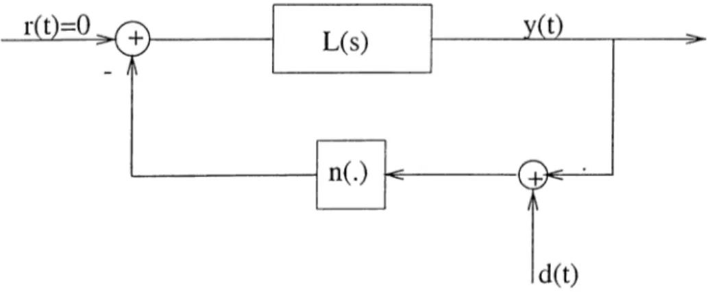
Dither is a high frequency signal, introduced into a system preceding the non­ linear element in an additive way in order to modify its nordinear characteristic. Figure 3.1 shows the configuration used for the application of dither. By sweep­ ing back and forth quickly across the domain of the nonlinecir element, dither

has the effect of averaging the nonlinearity, in a way inaking it smoother. Gen- ercilly, dither signals are ¡periodic deterministic or stationary random functions of time. Their frequencies are much higher than the system cut-off frequency so that they are filtered out before reaching the output. The application of var­ ious types of dither signals such as sinusoidal, triangular, square wave, random, etc. have been examined in the literature, see [18, 20, 21, 22]. The classiccil purpose of application of dither is the stabilization or elimination of limit cy­ cles in nonlinear systems. The cipplication of dither changes the behavior of a nonlinearity in the following wci.y.

Assume that n {.):R —> R is a memoryless nonlinearity satisfying the fol-

2' conditions:

• n

?r(0) = 0,

n(.) is Lipschitz, i.e. there is a constant 7 > 0 with the property I ?2(x) - n(y) \ < - f \ x - y \ V;r, y e R .

D e fin itio n : Let n (.):R —> R be a given function. The iimplitude distri­ bution function (ADF) of u(.) on a subinterval ( ^ ,¿2) of is defined cis the function Fy : R —> [0,1],

/i(f I t € ^'(0 — 0

M O =

{ t u h ) (3.1)

where y{.) denote the length in a Lebesque-measurable subset of R , see [23].

D e fin itio n :The function y (.):R —i· R is called F-repetitive, if there is a sequence 0 < ¿0 < h < ■■■ ■> unbounded from above, such that for i =

1, 2,..., the ADF of u(.) on ¿¿) equals the ADF of n(.) on (¿0, ¿1), see [23].

According to this definition, periodicity is not a necessary but a sufficient condition for F-repetitiveness.

When a fixed F-repetitive dither signal c/(i) is iipplied to a nonlinccirity ??-(.) satisfying the above conditions, the nonlinccirity becomes

n.

CO

(,t) = / - x)d(, (3.2)

where F^i^) is the derivative of ADF with respect to Further analysis on this property Ccin be found in [23].

In this work, the following piecewise constant periodic signal is taken as the dither signal.

d{t) = /?i kl' < t < («1 + k)T, /?2 (o!l + < t < («1 + Oi2 + k)7\ , k = 0 , l , . . . , (3.3) /dn ( S < t < {k + l)T. 2 = 1 n

where ¡3i G

Ft

In order to find the ADF of the function given by (3.3), let us construct two secpiences { a } and {/9}. These sequences are defined as { a } = {tt|,a2, ··· ,« n } and {¡d} = ■■■ 1 Pn)·, where o;;’s are the durations of difierent subintervals of one period of d{t) and ^¿’s are the magnitudes of d{l) corresponding to these subintervals. We can order {/?} to construct a new sequence [ft] = · · · , where (dj € {[d] and jdj < A if and only if j < i. Also, another new sequence {cv} is constructed where cck = aq with indices corresponding to jdu = (dj. If for any i , is deleted from the sequence, the corresponding dj is changed ¿is dj = dj + dj+i and dq+i is also deleted.

Using the definitions of { d } , {¡d} and ADF, the ADF of the signal given

by (3.3) is found to be, m ) = 0 —oo < ^ < /Si, di < /^2, ¿il + ¿^2 p2 ^ ^ < ^3)

m — 1

_

_

^ i

Pm — 1

^

l^ra-)

1

where rn is the number of entries of sequences { a } and { ^ }, and m < n.

Derivative of this function with respect to (f is,

^diO ~

~

Pi)

+ 0,'2(5(^ — ^

) + ··· + ««

^(

^ —

Pm)·,

where 6{^) is the impulse function. According to the property given in (3.2) a nonlinearity n{y) changes to n,.(y) as follows with the application of the dither signal (/(it) given by (3.4).

n.

.(y) =

Oiin[y

+

Pi)

+

Ci2n{y

+

P

)

+ ··· +

+

Pm)·

(’^•5)

n—1

+ /^i) + 1^2) + ··· + (1 “ <^i)'f'^{y + Pn)· i=l

Same result has also been found using a different methodology in [21].

Hence, the dither-applied system given in figure 3.1 is ecpiivalent to the system in figure 2.1, provided that the nonlinearity n{.) is replaced with the dither-applied nonlinearity n,.(.) given by the equality (3.7). The nonlinear­ ity n(.) should satisfy the conditions given at the beginning of this section to achieve this result. However, for chaotic systems and systems converging to a limit cycle, the Lipschitz condition can be weakened. Since such a system op­ erates in a bounded region, the input and output of its nonlinearity always stay in a bounded region. So, the nonlinearity is automatically locally Lipschitz.

Moreover, if the nonlinearity is differentiable and if'the solutions y remain in a bounded region i2, then an estimate of the Lipschitz constant 7 can be ob­ tained as:

see e.g. [24].

7 < sup I n'{y) j/efi

3.2

Application of Dither on the Control of

Chaotic Systems

Dither signal can be used to change many single input nonlinearities. However, the following control strategies are only applicable to systems in Lur’e form, given in figure 2.1, since they are mainly based on the conjecture of Genesio and Tesi which has been examined in the previous chapter. As mentioned in the introduction, control in the context of chaos means to force a chaotic system behave regularly (i.e. a limit cycle behavior) or conversely to force a regularly behaving system behave chaotically. In the following two strategies, in order to make a chaotic system exhibit a limit cycle behavior, the nonlinearity in the system is changed by the application of an appropriate dither signal so that the resulting system violates one or more conditions of the conjecture. Conversely, to make a regular system chaotic, the nonlinearity of the system is again changed by the application of an appropriate dither signal so that the resulting system satisfies the conjecture conditions more strongly. These two strategies have also been examined with application examples in [25]. In the third method the behavior of the system is observed from the bifuicatiou diagrams and one parameter of the system is changed by the application ot dither in order to make the system behave in a required way.

The control is applied as in figure 3.1, where the dither signal is given by,

d{t) , A; = 0,1,... , (3.8)

¡5i kT < t < {a + k)T, /32 {a + k)T < t < { k + 1)T.

for simplicity. The amplitudes /?i, /?2 and the duration a are chosen according to the desired effect. The frequency of the dither signal is not important, as long as it is more than three orders of magnitude greater tlian the operating frequency of the system.

3.2.1

Control Based on Equilibrium Point Elimination

According to the second condition of the conjecture, a system should have an unstable equilibrium point and according to the fourth condition, the location of that equilibrium point is close enough to the limit cycle for the system to exhibit chaotic motion. In this cipproach, the nonlinear element of the system with chaotic behavior is changed so that one or more of its equilibrium points are eliminated. The resulting system violates second and fourth conditions of the conjecture.

It is clear from equcition (2.11) that changing the nonlinearity ??.(.) of the system results in a change of equilibrium points. Nonlinearity changes as given by equality (3.7) when dither is applied. Equilibrium points of the resulting system can be found by solving

E + L(0)[cyn{E + /3i) + (1 - a)n{E + /^2)] = 0 . (3.9)

This equation can be solved analytically only in some special cases. However, it can easily be solved numerically or graphically in order to find the appropriate a and [3 values.

Application of an appropriate dither signal may eliminate the unstable equi­ librium point that interacts with the limit cycle. Existence and stability of a

limit cycle is not guaranteed for the dither-applied system. However, as men­ tioned before, the resulting system given by figure 3.1 becomes equivcilent to the original system given by figure 2.1, provided that the nonlinearity n(.) is replaced with n^f.). Hence, the describing function analysis and the conjecture are applicable to the dither-applied system and should be used to check the existence and stability of a limit cycle of the dither-applied system. In most ap­ plication examples, it has been observed that the dither-applied systems have stable limit cycles that Ccin be predicted with the describing function analysis.

3.2.2

Control Based on Interaction

This strategy is based on the fourth condition of the conjecture of Genesio and Tesi. According to the conjecture, if the interaction parameter r} is near unity, then the system may exhibit chaotic behavior. On the other hand, if ?/ is srncdl (i.e. near 0.5), then the system may exhibit regular motion. The interaction parameter is defined with respect to the equality (2.13). Since /1, B and E cire functions of dither parameters a, and ¡32 for the dither-a.pplied system, the amount of interaction can be increased or decreased by the application of dither. It is too difficult to analytically determine the dependence of 77 on dither parameters. However by fixing some of the dither parameters beforehand, other dither parameters can be found lor the desired r/ nurnericall}^ With this method by increasing 77, ci I'egular behaving system with an unstable equilibrium point and a stable limit cycle can be made chaotic, or a chaotic system can be forced to behave regularly by decreasing 77. After the parameters of dither are found, existence and stability properties for the dither-applied system should again be checked by describing function analysis.

This method results in complicated equations for an arbitrary nonlinearity n(.). If 7r(.) has a special structure (e.g. polynomial), then the analysis becomes

n/.) Figure 3.2: Compensating nonlinear feedback

much simpler. For more simplicity, assume that the chaotic system is given b}'

q{D)y{;t) + n{y{t)) = 0, (3.10)

where D is the differential operator q(.) and n{.) are polynomials of degree / cuid m respectively as given below.

q(s) — ¡)qS^ + ЬıS^' ^ + ... + 6/ -1.S + 6;, (3.11)

n{y) = «o2/ ”‘ + a iy”' ^ + ... + a,n-iy + а,„. (3.12) The system (3.10) can be transformed into the form given in figure 2.1, where L[s) = and ?г(.) is as given by (3.12). After the application of dither signal given by (3.8), the nonlinearity n(.) changes to

n._{■iy) =}

k = 0 i = 0

t.\

‘ /

(З.Ц)

Equality (3.13) can be simplified further, compensating the undesirable effects of dither by applying a polynomial output feedback and(or) a nonzero bias signal r(i) to the system as in figure 3.2, where /f,· gains can be found from (3.13) iis functions of a, and P2·

The resulting nonlinear block rir{y) is in iin espetially useful form such as, rir{y) == n{y) + a-2,13i..fh)y. (3.14)

The dither-applied system can be given as follows. When the modified nonlin- ecirity and the definition given by (3.11) are substituted in equation (3.10), we obtciin,

{boD‘ + h D ‘-^ + ... -b bi.,D + bi}y{t) + n{y{t)) + -0(a, A ,/^2)y(0 = 0, (3.15)

which yields,

+ biD^~^ + ... + bi-iD + (bi -b l3o ))]y{t) + n{y{t)) = 0. (3.16)

As can be seen from equation (3.16), the dither-applied system is equivalent to the original system with the only change being in 6/ which is the last term of the denominator q{s) of the transfer function of the linear block. The interciction parcimeter rj origincdly depends on system parameters, therefore on 6/. With this approach, the problem of choosing dither parameters to change y simplifies to the problem of choosing dither parameters to change 6/, which is simpler. yVlso, this approach gives the possibility of using bifurcation diagrams provided that the system behavior depends explicitly on bi.

For further special cases, n{y)=y^ and n[y)=y^, the above simplification ca.n be achieved without the use of compensating nonlinear feedback. For n(y)—y‘^, the modified nonlinearity becomes.

n.■iv) =y^ + ( « A + (i - «)/^2)j/ + (q'/^i + (1 - a)/3l). (3.17)

With the reference input,

r{t) = Kq = -(a /^ i + (1 - a)l5l) equality (3.17) is simplified to equality (3.14) where,

= a/3i + (1 — Ci);h·

When n{y)=y^, the dither-applied nonlinearity becomes,

ririy) = ;^'^ + (q:/?i + (1 —«)/^2)i/^ + (o!/^i+(1 —<^>')^2).!/ + ('^'^? + (*“ ‘^’'^)/^2)· (•^•171)

By selecting cv=0.5 and = equality (3.18) siiliplifies to equality (3.14) where,

^/^ = 0 .5 (A H ^ | ), without the need for a reference input.

3.2.3

Control Based on Bifurcation Diagrams

As mentioned before, bifurcation diagrams are used to show the changes in the behavior of a dynamical system with respect to a varying system parameter. Bifurca.tion dicigrams ot man}^ different chaotic systems can be found in the literature. Some examples are given in [16, 26].

Let a dynamical system have a system parameter which can be chcinged by the application ol dither without affecting the other parameters. Moreover, let the bifurcation diagrams ol this system with respect to this system pariirn- eter are available. Then the system can be forced to exhibit any behavior in those bifurcation dicigrams with the application of a suitable dither. Dither parameters are chosen to cluinge the required system parcuneter.

This strategy is applicable to a more general chiss of dynamical systems than the describing function analysis. However, it requires the knowledge of bifurcation diagi'iirns which mcxy be unavailable in some cases.

3.3

Application Examples

3.3.1

Chua’s Circuit

Ciuicx’s circuit given in figure 3.3 is a well-known nonlineiir electrical circuit that exhibits chaotic behavior for some parameter vcvlues, see [27]. Using Kir- choff’s laws and a little algebra, the governing equations of this circuit are Ibund to be, see [13],

.i’x — a { —Xi ,x'2 — n(,x'i)},

¿2 = X l - X2 + X3,

¿3 = -bX2,

(3.19)

where xi{t) = x^{t) =

and n{.) is defined as below. These equations can be transformed into a system in Lur’e form with the following linecir block and the nonlinear element,

+ .s + 6)

+ (1 + a)s^ + bs + ab^ (3.20)

(3.21) where y — x\ in (3.19). Chua’s diode has the characteristic i = n{ V) where n(.) is given as above. In this thesis as well as in other sources, the parameters of the nonlinearity are taken cxs ?ni - 0.286, m2 = 1.142 and M = 1.

P’igure 3.3: Chua’s circuit

Using the definitions (2.6) and (2.7), describing functions of the cxbove non­ linearity are determined as,

No{A, B) - - (m j -b m2) H---— B ( /0 ( — - — ] - }o B B N^{A,B) = - (m i -f m2) - b --- ^---( m 2 - mi f fi ( —[ A + M \ ) - /0 /A - M B B where. and = \ 1 + ( 1 - ^ ' ^ ) 2 1 1 1 ) 1 -2; | < 1 ; 1[ l · ^ · 1 1 1 > 1 . ✓ - 1 _{X < — 1 ,} f l { ^ ) = ^ f ( s i n - i ( . r ) ± a ; ( l - : r i ^ ) 5 ; ) 1 .T > 1 . (3.22) (3.23) (3.24) (3.2.3)

It is difficult to obtain analytical expressions lor limit cycle parameters /1, B and u. However, numerical solutions of (3.22-3.25) can easily be found for fixed a and b.

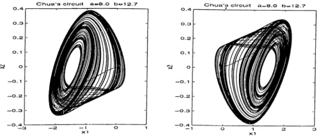
Chua’s circuit exhibits single scroll chaos for a - 8, and b = 12.7, see [13]. From the numericcil solution of (2.8-2.9) with (3.22-3.25), two limit cycles are predicted with A — ±1.0806, B = 0.9964 and cu = 2.335. These limit cycles are found to be stable according to the Loeb criterion.

This system has three equilibrium points at y - —1.5, 0, 1.5. The equilib­ rium point at ?/ = 0 is a separate equilibrium point and is unstable. It interacts with the predicted limit C3'^cles with 7/ = 0.922.

The linear block L{s) given by equality (3.20) hcis a moderate low pass lilter chciracteristic. According to the conjecture, this system may exhibit chaotic Ixehavior and simuhition results confirms this prediction. Two different chaotic attractors resulting from the interaction are shown in figure 3.4.

C h u a ‘3 c ir c u it a « S . O b*.12.7· C h u u ‘3 cIrcLJit a ^ B .O

Figure 3.4; Chaotic attrcictors of Chua’s circuit

This system is suitable for the application ol equilibrium point elimination. When the parameters of the dither signal given by equality (3.8) a.re chosen as a = 0.5, /3i = 0.1 and /^2 = —0.5, the nonlinearity n(-t/) changes as shown in figure 3.5. From the crossings of the modified nonlinearity with the line which is shown cis the dotted line in the same figure, it is found out that the dither-ajDplied system has one equilibrium point at ?/ = —2. So, the equilibrium point at y = 0 is eliminated.

Original nonlinoarily Modiliod nonlinearity

Figure 3.5: Chua’s nonlinearity before and after the application of dither

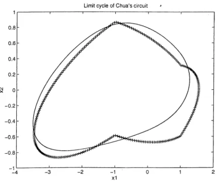
Describing function analysis predicts a stable limit cycle for the ditlier- applied system, which is plotted in figure 3.6 by plus signs. Simulation of the dither-cipplied system also gives a limit cycle at the same region, wliicli is shown as the solid line in the same figure. The predicted and actiud limit cycles are not cjuite close. This difference is due to the approximation errors of the describing function analysis, since the linear block L(s) given by equality

Limit cycle of Chua's circuit

Figure 3.6: Actiuil and predicted limit cycles of Chua’s circuit after the appli­ cation of dither

(3.20) does not have enough filtering effect.

3.3.2

Relay System

This is a third order system given in Lur’e form as in figure 2.1 with,

1 L(,s) = -f + 6s -f- c ’ 1 ;(/ < 0 < 0 y = 0 - 1 y > 0

Describing functions of this nonlinearity are given in [16] as, 2T No(A,B) = iV i(/l,5 ) = -7T/1 4 cos T (3.26) (3.27) ttB (3.28) (3.29) 24

where \I/ = -!

-7t/2 A < - B a,rcs'm{A/B) |A/B |< 1 7t/2 A > B

The solution of (2.8) and (2.9) for these functions yields

B = — .S'-' -7TC

_V

_V

S ta te d iag ra m of relay sys te m for a=1 ,b = 2 .5 ,c = 4

^ 0

- 0 . 4 - 0 . 2 0 .2 0 .4 0 .6

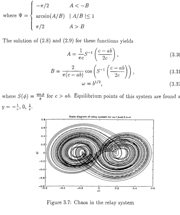
Figure 3.7: Chaos in the relay .system

For parameter values a = 1.0, 6 — 2.5, c = 4.0, this .system exhibits double scroll chaotic motion as can be seen from figure 3.7. The equalities (3.30-3.32) for the.se parameter values show two predicted limit cycles with A = ±0.3434, B = 0.3498, u> = 1.5811. The stability of these limit cycles cannot be ancilyzed l:>y the Loeb criterion, however in [16] it is shown that the limit cycles are stable. The equilibrium point at ?/ = 0 is unstable and intercicts with the predicted limit cycles with rj = 0.9817. The linear part L{s) of the system given by equality (3.26) has suitable filtering effect. Hence, this system satisfies the conjecture given in chapter 2.

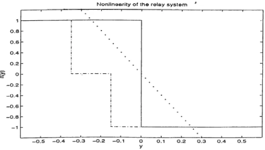
N o n lin e a r ity o f th e re la y s y s te m

E'igure 3.8: Nonlinearity of the relay system before and after the application of dither

Although the nonlinearity n(y) given by equality (3.27) is not Lipschitz and does not satisfy the conditions for dither given at the beginning of this chapter, the application of dither to relay type nonlinearities has been analyzed in [18, 20]. The application of the dither signal given by (3.8) with a = 0.5, Pi = 0.15 cuid /?2 = 0.35 changes the nonlinearity as in figure 3.8. In this figure the solid line represents the original, the dcish-dotted line represents the modified nonlinearities. The dotted line is As can be seen from the crossings, the dither-applied system has one equilibrium point at y = —\i so the equilibrium point at ?/ = 0 has been eliminated.

R e la y s y s t e m --- a c tu a l + + -e p re d ic to d lim it c y c le s

Figure 3.9: Actual and predicted limit cycles of the relay system alter the application of dither

In figure 3.9, the actual limit cycle found from tile sirnuhitions is shown cis the solid curve. The predicted limit cycle found from the describing function analysis is cilso given in the same figure plotted with plus signs.

3.3.3

System with a Square Nonlinearity

Consider the nonlinear differential equation,

ii + ay + by + cy + 1/ = 0.

This equation can be turned into a system in Lur’e form, with

L(s)

=

‘

Describing functions for this nonlinearity and the corresponding limit cycles are found as,

(:;i.36) (3.37)

=

,

A = — r —

.

2

This system has one limit cycle which is stable ciccording to the Loeb cri­ terion. Also, the linear part of the system has suitable filtering effect. Two equilibrium points are found at y = 0, —c. The separate equilibrium point at y = —c is unstable for c > 0 and interacts with the limit cycle with

c — ab. ,1 =

c ab (3.38)

This system e.xhibits chaos for parameter values a = 0.4, b = 1.18, c = l.O, .see figure 3.10. The equalities (3.37) and (3.38) for these piirameter values show that this system obeys the conjecture given in the 2nd chapter with 7/==0.846. Since interaction parameter r/ for this system system is a function of system parameters, the system is suitable for the application of control

C h a o s in th e s q u a r e n o n lin e a rity system ^

0 .2 0 .4

Figure 3.10: Chaos in the system with square nonlinearity

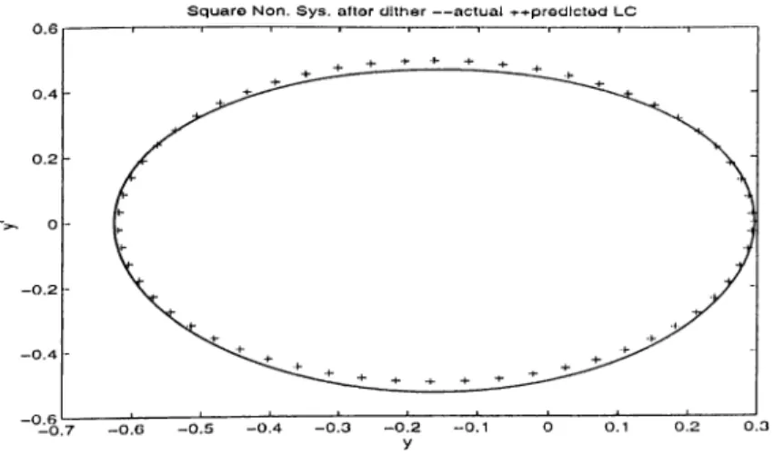
based on interaction. The nonlinearity is a square polynomicil, therefore dither parameters can be selected in order to change c and decrease t]. The application of the dither signal given by equality (3.8) for a = 0.5, /?i = —0.3 and /^2 = 0.1 and a constant reference input r{t) — 0.05, decrease rj to 0.515. Simulation of the system after the application of this control shows the e.xistence of a stable limit cycle which can be predicted by the describing function analysis quite precisely. The actual (solid curve) and predicted (plus signs) limit cycle of the control applied .system are shown in figure 3.11.

S q u a r o N o n . S y s . a fto r d ith a r — a c tu a l ^ -t-prodlc tod L C

Figure 3.11: Actual and predicted limit cycles of the system with square non­ linearity after the application of dither

Conversely, for parameters a = 0.4,6 = 1.18 and c = 0.8, the system exhibits a limit cycle behavior. Desci'ibing function analysis shows an interac­ tion of r) = 0.515. This time by applying a dither signal to the system with a = 0.5, = —0.15 and ^2 = 0.35, and also a constant reference input as r(i) = 0.0725, the interaction cimount is increased. The resulting system with rj = 0.85 exhibits chaotic behavior.

3.3.4

System with a Cubic Nonlinearity

In this example, the following nonlinear differential equation is considered, see [15],

y' + ay -I- by + cy + 1/ = 0. This system can also be turned into the Lur’e form, with

1

(3.39)

^ ^ + a.s^ + 6.S -r c ’ n{y) = t/.

The corresponding describing functions are found as,

No{A,B) = A^ + r^B'^ , i\h(A,B) = 3A^ + ^B\

(3.40)

(3.41)

(3.42

The limit cycles of this system are predicted with the following parcvmeters.

1

These two predicted limit cycles are stable due to the Loeb criterion. This system hcis three equilibrium points at ?/ = 0, for c < 0. The equilibrium point at ?/ = 0 is unstable. Also, there is suitable filtering effect on the system.

S y s te m w ith th e c u b ic n o n lin e a rity — c h a o ^

Figure 3.12: Chaotic behavior for the system with cubic nonlinearity.

The interaction parameter is ?; = 0.873 for parameter values a = 1.0, 6 = 1.5 and c = —1.25. For the.se parameters, this .system exhibits a double scroll chaotic behavior, shown in figure 3.12.

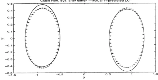
Using the control based on interaction strateg}'· described in the previous section, dither parameters in equality (3.8) are chosen as a = 0.5, fi\ = 0.65,

^2 = —0.65, yielding rj = 0.395. Simulation of the dither-applied system shows two symmetric stable limit cycles, which can be predicted with the describing function analysis. Actual (solid curve) and predicted (plus signs) limit cycles are shown in figure 3.13.

Cubic Non. Sys. after dither---actual predicted LC

Figure 3.13: Limit cycles for the S3^stern with cubic non. after the application of dither.

3.3.5

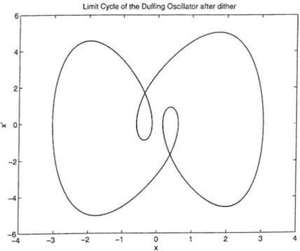
Duffing Oscillator

Duffing oscillator is a forced oscillator that is used extensive)}^ in nonlinear studies, since it can describe many physical phenomena, see [26, 28]. The governing equation for this system is.

x-\- aix + aox + x^ = qcos{u;t) + tt{t)

This equation can be turned into Lur’e form with,

L{s) = -- --- ---, S -f- -|- CLq n{y) = 2/^ r{t) = ^cos(cui) + u{t). (3.46) (3.47) (3.48) (3.49)

SBDF cannot be cipplied to this system because of the forcing term. How­ ever dither Ccui be applied to the nonlinearity given by equality (3.48) as it luis been done in the previous section.

For this system, from the bifurcation diagrams civailable in the literature, [26, 28], we choo.se two parameter sets;

Set 1: ao=0, ai=0.25, q = l l , cu=l. Set 2: ao=0.64, ai=0.25, q = l l , u>=l.

It is known that this .system exhibits a chaotic behavior for the first pcirameter set and a limit cycle behavior for the second parameter set. It is obvious that by changing the parameter ao effectively, we rnciy switch the behcivior of this sj^stem from chaotic behavior to limit cycle behcivior, and vice versa. This effective change can be achieved by applying a suitable dither signal.

Choosing the dither pcirameters as cv=0.5, /3i=-0.8 and /32=0.8, we nuvy chcinge the parcimeter ciq from «o = 0 to ao = 0.64. Hence, although the system with the parameters given in Set 1 exhibits cluiotic behavior before the application of dither, it exhibits the limit cycle behavior dictated by the

parameter set 2 after the application of dither. This point is confirmed with the simulation results as shown in figure 3.14 and figure 3.15.

Chaos in the Duffing Oscillator

X 0

Figure 3.14; Chciotic behavior of the Duffing oscillator

Figure 3.15: Inmit cycle for the Duffing oscillator after the application of dither

Chapter 4

Observer Based Feedback

Control of Chaotic Systems

4.1

Observers

In many physical systems, all state variables are not directly available as output signals. However, in some situations, especially for state feedback control, a knowledge of state values is required. Some sort of ad hoc differentiation of measured states may provide an estimate of the unmeasured states. This method does not give accurate performance in many crises, especicilly in the case of noisy data. A better way is to use the full knowledge of the mathematical model of the system with the available output in order to estimate the unknown states. The resulting estimator system is Ccilled an observer. In this work, full state observers that produce estimates of all state variables are considered.

The theory of observers for linear systems is well-developed. In order to reach a theory for nonlinear s}^stems, one should begin with linear systems.

4.1.1

Linear Observers

(4.1) Consider a dynamical system described by the equations

X — Ax + Bu, у = Cx.

where x is an n x 1 vector consisting of system states, A G В G C G are constant matrices, и is the input and у is the output of the system. A well-known fact for this system can be stated as follows:

T h e o r e m : Бог the above system, the following conditions are equivalent.

i The pair (C, /1) is observable.

ii rank[C/^ /F C '^ . . . = n.

iii For any real and monic polynomial p(A) of degree ?r, there exists a con- stcint matrix

K G R"""™ such that det(A / - /1 + K C ) = p(A).

P r o o f :See e.g. [29].

For a linear dynamical system given by (4.1), if the pair (C, /1) is ob.servable, an observer system that can estimate all states of the original system can be constructed as,

X = Ax + K {y - y ) B Bu, y = Cx.

where K G R"^™ will be chosen accordingly.

Defining e = x — x, we get an error system between the states ot the original system and the observer as,

é = { A - K C )e - /F e (4.3)

From the theorem stated cibove, K can be chosen such that the eigenviilues ol /[^ — /{ — }\C all hcive negative real parts. Then the error ec[uation becomes

exponenticilly stable, indicating that,

e(t) —> 0 or x{t) x[t) as t —> oo.

This class of observers can be generalized to a class of nonlinear dynamical systems, namely for nonlinear dynamical systems that are linecU’ up to cin output injection. Consider the dynamical system of the form.

X — Ax + g{y) + Bu. у = Cx.

(4.4)

In this class of nonlinear dyncimical systems, only the output signal is sub­ jected to a nonlinearity. Since the output is available from the original system, we may still use cin observer similar to the one given by (4.2).

Let the observer system be,

X = Аг- 4- K{;y - y) -f (j{y) -b Bu, у = Cx.

Defining e = X — x, as for the linear case, we get the error system as,

i = { A - K C )e = A e

(4.5)

(4.6)

with an appropriate choice ol A G such that Ac is a Hurwitz matri.x, it follows that the error e{t) decays to zero e.xponentially fast.

Note that systems in Lur’e form are linear up to output injection. To see this, consider the standcvrd Lur’e system given by figure 2.1. Let {A ,B ,C ) be a mininml state representation of L{s), i.e.,

L{s) = C {s l - A)-^B

and (C, /1) is observable. Then, a state space representation of the system given in figure 2.1 can be given as.

X = Ax — Bn{y), у = Cx.

35

Hence, the observer given by (4.5) can be used to Estimate the states of any system in Lur’e form.

Yet, observer for a more general class ol nonlinear dynamical systems which are given by the following equations can be constructed.

■i- = Ax + g[x) + Bii, y = Cx,

where the nonlinearity is Lipschitz, i.e.

II

six) -

</(-co) II < 7 II - .To II

For the design methodology and analysis of such observers, see [30].

(4.8)

(4.9)

4.2

Observer Based State Feedback Control

of Chaotic Systems

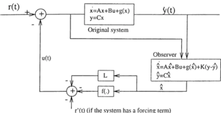
Feedback control of chaotic systems is not a new subject. It has been excirnined in the literature, see [6, 12]. In these articles only one system. Duffing oscillator has been considered. In [12], an observer different from the one given by (4.5) is considered. However, a general state feedback control scheme should be based on a general observer scheme, since in most practical situations, system states Ccinnot be measured directly.

Consider a system given by the equation (4.8). A generiil feedback control law based on an observer for this system can be given as.

u{t) = Lx(t) -t- f{ x {t)) , (4.10)

where x is a vector consisting of observer states, L G is the feedback gciin matri.x and / ( . ) is the nonlinear feedbcick gain function. With the suitable choice of L and / ( . ) , the system given by (4.8) can be controlled (i.e is forced

Figure 4.1: Feedback based on observer configuration

to behave regularly or chaoticcdly according to the purpose). The configuration shown by figure 4.1 is used to apply the control law. If the system is a forced system, then a forcing term can also be included in (4.10) to cancel it.

In the following sections, two different strategies will be examined in order to choose L and / ( . ) for different types of systems.

4.2.1

Feedback Control Based on Interaction

Assume that the system given by (4.8) is a system to which the analysis method and the conjecture given in chapter 2 are applicable. The system should be in Lur’e form, therefore is automatically linear up to output injection. An oliserver of the form given by (4.5) can be constructed for it.

(4.11) Consider the following feedback law,

■«(i) = Lx{t)

is applied to this system. The resulting system becomes, X = (/1 — B L )x + (/{y) + BLe, y - Cx,

where e = .c — x is the observer error. Since e{t) decays to zero exponentially feist, we may neglect the term BLe in (4.12). Hence, the representation ot the

37

system in Lur’e form as given by figure 2.1 becomes, L{s) = C {sI - A +

nfe) = »(>/)■

(i.l3)

The interiiction parameter rj for this system can be calculated analytically or numerically. This parameter will in general be a function of the feedback gciin matrix L. Therefore, by adjusting the feedback gain L, we mciy also adjust the amount of interaction This way we may force the system to change its behavior from chaotic motion to reguhir motion, or vice versa.

4.2.2

Feedback Control Based on Bifurcation Dia­

grams

Consider the system given by (4.8). Assume that for such a system an observer can be constructed so that the observer states x{t) converges e.xponentially to the original system states, x{t). Then, we may use a state feedback law as given by (4.10). Hence the state space representation of the system becomes.

.T = (A - BL)x + i g - f ) { x ) + BLe + h(e), (4.14)

where e = x — x is the observer error, {g — / ) ( . ) is the resulting nonlinearity and h{e) - g{x) - f { x ) - [g ~ f)(x )· Since e{t) decays exponentially to zero, we may neglect the term BLe in (4.14). Choosing / ( . ) appropriately, in some cases, we may also make h{e) to decay zero or in other cases choosing / ( . ) = 0, we may keep {g - f ) { x ) = g{x) and h{e) = 0. Therefore, with the ¿rppropriiite choice of L, some of the entries of the matrix A of the original system can be changed.

Assume tliat the system parameters corresponding to the entries that can be changed by L or by / ( . ) determine the dynamical behavior of the system given by (4.8). Also, assume that bifurcation diagriims in terms ol some ot

these parameters are available. Then by choosing the appropriate feedback law given by (4.10), we may change the behavior of the system to one of the behaviors shown in the bifurcation diagram. This kind of control on a special class of chaotic systems, namely forced chaotic oscillators has been examined in [31].

4.3

Application Examples

4.3.1

Chua’s Circuit

Chua’s circuit can be transformed into Lur’e form and describing function analysis can be applied to it as it has been examined in section 3.3.1. Therefore, it is a good candidate for the feedback control based on interaction.

Consider the system given by equations (3.19). VVe construct an observer oi the form given by equations (4.5) for this system using the following observer gain matrix. K = 5f>-6 \ α^ a — b+6 4q —α^ —46 (4.f5) /

This observer gain matrix locates the eigenvalues of Ac = A — K C at A = — f, —2, —3. Since, Ac is stable, the observer states given by (4.5) converges to the states of the originell system.

This .system exhibits chaotic behavior for a = 8.0, b = 12.7, as shown in figure 3.4. The interaction pcirameter for the original system is r/ = 0.922. A feedback law for this system is chosen as.

u(i) — l\Xi(t) + l2'X2{t^ "h C*^.3(0 (4.16)

The feedbcick gain parameters for the closed loop system are found to be,

Feedback applied Chua's circuit

Figure 4.2: Limit cycle of the Chua’s circuit after feedback is applied

= —0.2, /2 = 1-0 and /3 = 0.2, in order to set the interaction parameter Tj = 0.5. The resulting limit cycle of the feedbcick applied system is .shown in figure 4.2.

4.3.2

Relay System

Relay system examined in section 3.3.2 is another good candidate for the ap­ plication of observer based state feedback control by changing the interaction parameter. A state space representation for the relay system given by equations (3.26) and (3.27) is found as.

Xl = X2,

¿2 = X3,

¿ 3 = - c x i - bx2 - ax3 — n ( x i ) .

:4.17)

where n(y) is givom by (3.27).

In terms of the system piirameters, an observer for this system can bo

constructed with an observer gain matrix, /

K =

6 — a

11 — 6a + — 6

6 — 11a + Ga"^ — a^ + 2ab — 6b — c

in order to put the eigenvalues of the matrix Ac = A — K C at X = —3. Hence, the observer error e(t) decciys exponenticdly to zero.

(4.18)

-

1

,

- 2

,

As it has been shown in section 3.3.2, for parameter values a = 1.0, 6 = 2.5 cind c = 4.0, this system exhibits a chaotic motion of the form given by figure 3.7. The interaction parameter corresponding to this motion is r/ = 0.9817.

When a feedback law of the form given by (4.16) is applied to this system with /i= 0 , /2=10 and /.3= -0.8, the system e.xhibits a limit cycle behavior as can be seen from figure 4.3. The feedback parameters are chosen such that the interaction partimeter of the feedback applied system becomes ?/=0.5.

Feedback applied relay system

Figure 4.3: Limit cycle of the relay system after feedback is applied