ГГ',-Jf-ni. ^ ''Г*, · ' Г Г-' «у-. 1^ .■ r ~ . ''· Ή ‘ ' '· , ^Г ."Τ'-i ' · • /* f '*''
THE ESTIM ATORS OF RANDOM COEFFICIENT MODELS
The Institute of Economies and Social Sciences of
Bilkent University
by
YASFMiN BALGUNDUZ
In Partial Fulfillment of the Requirements for the Degree ol' DOCTOR OF PHILOSOPHY IN ECONOMICS
m
THE DEPARTMENT OF ECONOMICS BILKENT UNIVERSITY
ANKARA
6^A
• G S í
I certify that I have read this thesis and have found that it is fully adequate, in scope and in quality, as a thesis for the degree of Doctor of Philosophy in Economics
I certify that I have read this thesis and have found that it is fully adequate, in scope and in quality, as a thesis for the degree of Doctor of Philosophy in Economics
■ ^
Asst. Prof Dr. Kıvılcım Metin Examining Committee Member
I certify that I have read this thesis and have found that it is fully adequate, in scope and in quality, as a thesis for the degree of Doctor of Philosophy in Economics.
Asst. Prof. Dr. Turan Erol Examining Committee Member
I certify that I have read this thesis and have found that it is fully adequate, in scope and in quality, as a thesis for the^egfee of Doctor of Philosophy in Economics
Asst. IW f Dr. Mehmet Caner Examining Committee Member
I certify that I have read this thesis and have found that it is fully adequate, in scope and in quality, as a thesis for the degree of Doctor of Philosophy in Economics.
Asst. Prof Dr. Aslihan Salih Examining Committee Member
Approval.of the Institute of Economics and Social Sciences
Prof Dr. Ali L. Karaosmanoğlu 7· Director
ABSTRACI'
THE ESTIMATORS OE RANDOM COEFFICIENT MODELS Bal Gündüz, Yasemin
Ph.D., Department of Economics Supervisor: Prof. Dr. Asad Zaman
June 1999
This thesis concentrates on the estimators of Random Coefficient models. A Bayesian estimator with non-standard posterior density implementing Griddy Gibbs Sampler technique for 1 lildreth-Mouck type Random Coefficient Model is introduced and it is compared with a range of existing estimators for Random Coefficient models. Monte Carlo experiments are used for comparing this estimator with Swamy and Tinsley (1980), Method of Moments and Zaman (1998) Modified Maximum Likelihood estimators on the basis of biases. Mean Square Errors and efficiencies of parameter estimates. The results show that performances of estimators are affected by sample size, balance of design matrix and variance structure of stochastic regression coefficients. In most of the cases estimates for variance parameter of regression coefficients are seriously biased for all estimators except the Bayesian Griddy Gibbs estimator. The Bayesian Griddy Gibbs and Method of Moments estimators show better performance compared with others, the best one changes in lines with some observable and unobservable criteria. In empirical work, using both methods in estimation and selecting the estimates with minimum out of sample forecast Mean Square Error might be recommended. Asymptotically Maximum likelihood estimator is unbiased and achieves Cramer Rao Lower Bound therefore it can not be improved upon. The finite sample properties of Modified Maximum Likelihood estimator are studied with a separate Monte Carlo study and it is shown that except very high sample sizes relative to the dimension of the problem there is substantial room for improvement of the of Modified Maximum Likelihood estimator in finite samples.
Key Words: Random Coefficient Model, Griddy Gibbs Sampler, Maximum Likelihood , Method of Moments, Monte Carlo Experiment, Bayesian Methods
OZE'r
STOKASTİKKAFSAYILI MODI-LLİİR İÇİN TAHMİN YÖNTEMLERİ
Bal Gündüz, Yasemin Doktora, Ekonomi Bölümü Tez Yöneticisi: Prof. Dr. Asad Zaman
Haziran 1999
Bu tez Stokastik Katsayılı modellerin tahmin yöntemleri konusunu ele almaktadır. Hildreth-Houck tipi Stokastik Katsayılı model için Standard olmayan veri sonrasal (posterior) frekans dağılımlarından örneklemeyi sağlayan “Aralıksal Gibbs Önıekleyicisi” tekniğini kullanan bir Bayesyen tahmin yöntemi geliştirilmiştir. Monte Carlo deneyleri kullanılarak bu yöntem literatürde önerilen Svvamy ve Tinsley(1980) yöntemi, Momentler yöntemi ve Zaman(1998) ile önerilen “Değiştirilmiş Olabilirlik Maksimizasyonu” yöntemi ile karşılaştırılmaktadır. Karşılaştırma kriterleri yanlılık, gerçek parametrelerden sapma kareleri ortalaması ve etkinliktir. Tahmin yöntemlerinin performanslarının örneklem büyüklüğü, açıklayıcı değişkenler matrisinin dengesi ve stokastik katsayıların varyans yapısından etkilendiğini görülmektedir. Bayesyen yöntem dışındaki yöntemler için stokastik katsayıların varyans parametresi tahminleri belirgin biçimde yanlıdır. Bayesyen yöntem ve momentler yöntemi diğer yöntemler ile karşılaştırıldığında daha iyi performans göstermektedir. En iyi yöntem bazı gözlemlenebilir ve gözlemlenemez kriterlere bağlı olarak değişmektedir. Ampirik çalışmalarda her iki yöntemin uygulanması ve örneklem dışı gözlemler için en düşük ortalama öngörü hataları karesi veren yöntemin seçilmesi önerilmektedir. Asimplotik olarak Olabilirlik Maksimizasyonu yönteminin yansızlığı ve kovai-yans tahmininde Gramer Rao alt sınırına ula.şacağı bilinmektedir. Bu çalışmada Olabilirlik Maksimizasyonu yönteminin sonlu örneklem boyutu özellikleri ayrı bir Monte Carlo deneyi ile araştırılmaktadır. Sonuçlar problem boyutuna oranla çok büyük örneklem boyutları dışında bu yöntemin performansının alternatif tahmin yöntemleri ile belirgin olarak iyileştirilebileceğini göstermektedir.
Anahtar Kelimeler: Stokastik Katsayılı Model, Aralıksal Gibbs Örnekleyicisi, Olabilirlik Maksimizasyonu Yöntemi, Momentler Yöntemi, Monte Carlo Deneyi, Bayesyen Yöntemler
I would like to express my gratitude to Prolessor Asad Zaman lor his invaluable supervision. I am indebted to him for his very valuable suggestions at times that I most needed and constant support during this study. Special thanks go to professors Kıvılcım Metin, Turan Erol, Mehmet Caner and Aslıhan Salih for their careful reading and valuable comments.
Parts of this thesis were presented at the 1997 International Symposium on Forecasting and 1998 METU International Conference on Economics. 1 wish to thank to the participants in these meetings. Papers originating from this thesis will also be presented at the 1999 International Symposium on Forecasting and 1999 Econometric Society Australasian Meeting.
I would like to express my special thanks to Undersecretariat of Treasury Deputy Undersecretary Cüneyt Sel, Deputy Undersecretaiy Ferhat Emil, General Director Dr. Özhan Üzümcüoğlu and Deputy General Director Murat N. Arikan for their great support during this study. My special thanks must also go to my colleagues at the Undersecretariat of Treasury, who are too numerous to mention here, for providing me with their computer facilities, which made the simulation experiments in this thesis manageable.
Acknowletigcincnts
I am grateful to my mother and fatlier for their aflection, support and great encouragement throughout my life and especially during this study. Finally I am especially thankful to my husband Eriş for his invaluable support, patience and encouragement.
I'ABLl· Ol·' CON l i'N I S ABSTRACT...·... iii ÖZET... ... iv ACKNOWLEDGEMENTS... v TABLE OF CONTENTS... vi LIST OF TABLES... ix LIST OF FIGURES... x CHAPTER 1: INTRODUCTION... 1
CHAPTER 2: LITEIL\TURE REVIEW... 5
2.1 The Hildreth-Houck(l968) Random Coefllcient M odel... 8
2.2 Theoretical Arguments for the Random Coefficient Specification... 11
2.3 Random Coefficient Approach and the Bayesian Perspective... 15
2.4 Estimators for the Random Coefficient Models and Pioneering Monte Carlo Comparisons... 19
2.5 Sampling Based Approaches: Gibbs Sampler Technique and Griddy Gibbs Sampler Technique... 26
CHAPTER 3: SOME ESTIMATORS FOR RANDOM COEFFICIENT MODELS PROPOSED IN THE LITERATURE... 29
3.1 The Modified Maximum Likelihood Estimator (M M L)... 30
3.1.1 The Inconsistency of MI... 31
3.1.2 The Modified M L ... 32
3.3 The Swamy and Tinsley Estimator (SWAMSLEY)... 33
CHAPTER 4: INTRODUCTION OF NEW ESTIMATORS FOR RANDOM COEFFICIENT M ODELS... 37
4 .1 The MOM Estimators... 38
4.1.1 The Boundary Permutations M O M ... 39
4.1.2 The Constrained MOM Estimator... 39
4.2 Bayesian Estimators Implementing Gibbs Sampler... 40
4.2.1 Bayesian Estimator with Standard Posterior Densities... 40
4.2.2 Bayesian Estimator with Non-standard Posterior Densities: The Bayesian Griddy Gibbs Estimator... 44
CHAPTER 5: MONTE CARLO COMPARISONS OF ESTIMATORS FOR RANDOM COEFFICIENT MODELS... 49
5.1 Design of the Monte Carlo Study... 50
5.2 Monte Carlo Results... 53
5.2.1 The Bayesian Griddy Gibbs Estimator (The Bayesian G G )... 54
5.2.2 Swamy and Tinsley Estimator (SWAMSLEY)... 55
5.2.3 Modilled Maximum Likelihood Estimator (M M L)... 57
5.2.4 Method of Moments Estimator... 58
5.3 Conclusion... 60
CHAPTER 6: FINITE SAMPLE PROPERTIES OF FHE MODIFIED MAXIMUM LIKEUHOOD ESTIMA FOR: A MONTE CARLO EXPERIMENT... 70
6.2 Results... 74
6.2.1 Bias and Eniciency of β Estimates... 74
6.2.2 Bias and EBiciency of λ E.stimates... 83
6.3 Conclusion... 91
CHAPTER 7: CONCLUSION... 93
SELECT BIBLIOGRAPHY... 101
APPENDIX A (Tables A. 1 -A. 10)... 106
LIST OF TABLES
Table 5.1. The Monte Carlo set-up... 52
Table 5.2. MSB of >9estimates (% Difference from the True;i GLS)... 62
Table 5.3. MSB of A estimates (Ratio to the method with the minimum MSB of X in each case)... 63
Table 5.4. Bfficiencies of estimates (Ratio to the efficiency of'frue X GLS)... 64
Table 5.5. Control variate regression results for MSB o festim ate s (% Difference from the minimum among (hem)... 66
Table 5.6. Bias ofp estimates... 67
Table 5.7. Bias of/1 estimates... 68
Table 5.8. Number of multiple solutions by S WAMSLBY... 68
Table 6.1. The Monte Carlo set-up for the design matrix... 73
Table 6.2. Response surface regression results for the bias of X estimates for MML and M OM ... g4 Table A. 1. The MSB of y? - Untruncated Results... ... ] 06
Table A.2. The MSB of X - Untruncated Results... 107
Table A.3. The Bfficieneies of p - Untruncated Results... 108
Table A.4. The Results of control variate regressions for p -Untruncated Results... 110
Table A.5. The Bias of T - Untruncated Results... 112
Table A.6. The MSB of y^- Truncated Results... 113
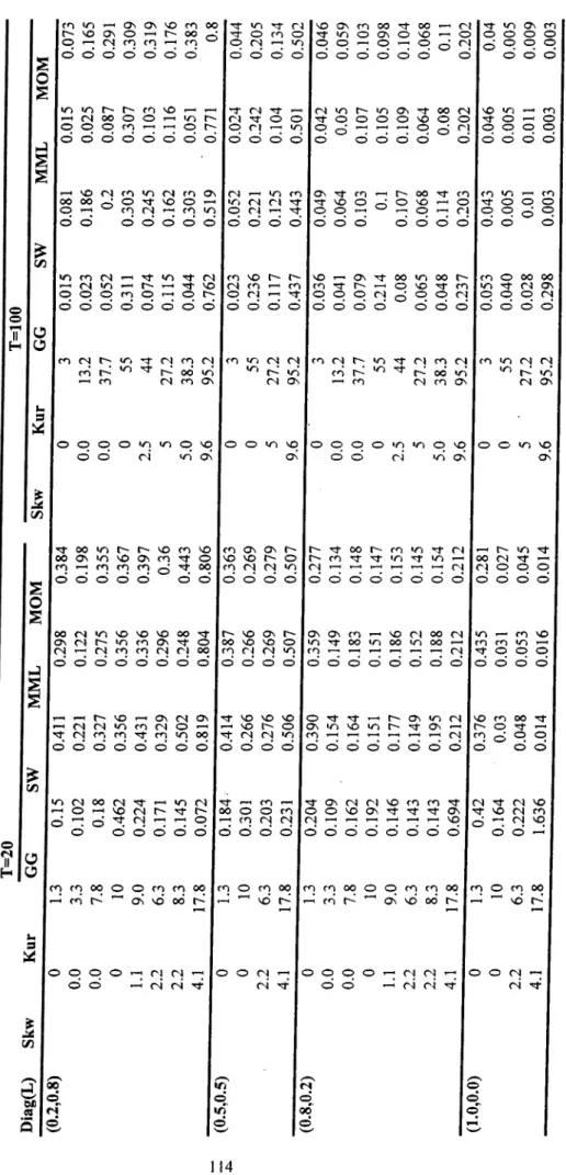
Table A.7. The MSB o f X- Truncated Results... 114
Table A.8. The MSB o f X- Truncated Results... 115
Table A.9. The MSB o f X- Truncated Results... 116
LIST OF FIGURES
Figure 5.1 Illustration of boundary maximization... 69 Figure 6.1 The MSB of ¡3 estimates for the MMT versus
MOM-% Difference from TRUGLS... 79 Figure 6.2 The Efficiencies of TRUGLS versus
MML-The effect of sample size... g I Figure 6.3 The Efficiencies of TRUGLS versus
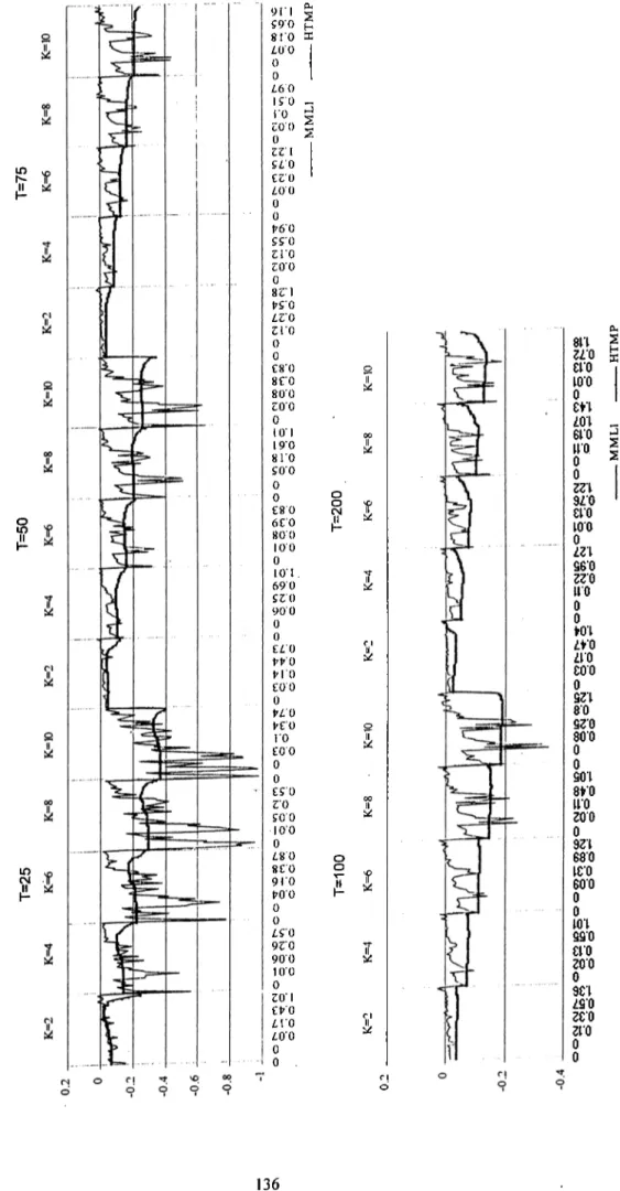
OLS-The effect of parameter variation... 82 Figure 6.4 Bias of X estimates for MML and MOM... 85 Figure 6.5 The ratio of the MSE of X estimates with MML
to the MSE of X estimates with MOM... 89 Figure 6.6 The MSE of X estimates with MOM versus the MSE of
X estimates with OLS... 90
Figure B1 Biases of estimates with MML and MOM... 120 Figure B2 The Efficiencies of TRUGLS versus
MML-Square root of the ratio to the CRLB... 121 Figure B3 The Efficiencies of TRUGLS versus
MOM-Square root of the ratio to the CRLB... 126 Figure B.4 The Response Surface Fit between the bias ol' T, (MML)
and the Lambda Polinomial... 129 Figure B.6 The Response Surface Fit between the bias of A, (MOM)
and the Lambda Polinomial... .. Figure B.7 The Response Surface Fit between the bias of T, (MOM)
and the Lambda Polinoniial... j Figure B.8 The Response Surface Fit between the bias of A, (MML)
and the Kurtosis Polinomial... Figure B.9 The Response Surface Fit between the bias of A^ (MML)
and the Kurtosis Polinomial... I33 Figure B.IO The Response Surface Fit between the bias of A, (MOM)
and the Kurtosis Polinomial... I34 Figure B.l 1 The Response Surface Fit between the bias of T,(MOM)
and the Kurtosis Polinomial... I35 Figure B.12 The Response Surface Fit between the bias of A, (MML)
and the heteroscedasticity measure... I35 Figure B.13 The Response Surface Fit between the bias of T, (MML)
and the heteroscedasticity measure... I37 Figure B .l4 The Response Surface Fit between the bias of A, (MOM)
and the heteroscedasticity measure... 138 Figure B .l5 The Response Surface Fit between the bias of A, (MOM)
and the heteroscedasticity measure... I39 Figure B .l6 The Response Surface Fit between the bias of A, (MML)
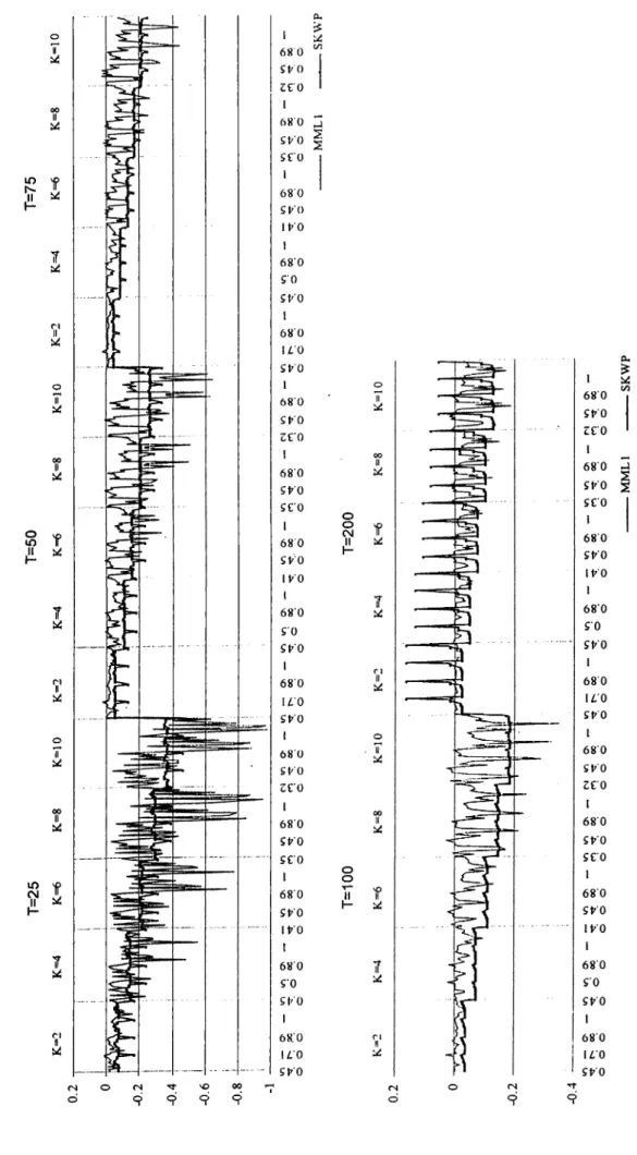
and the Skewness Polinomial... 140 Figure B.5 The Response Surface 1-il between the bias of
A,
(MML)and the Skewness Polinomial... 141 Figure B.18 The Response Surface Fit between the bias of A, (MOM)
and the Skewness Polinomial... ... . ¡42 Figure B. 19 The Response Surface Fit between the bias of T,(MOM)
and the Skewness Polinomial... I43 Figure B.20 The Response Surface Fit between the bias of A, (MML)
and the Correlation of Regressors... 144 Figure B.21 The Response Surface I'it between the bias of Tj (MML)
and the Correlation of Regressors... ... 145 Figure B.22 The Response Surface Fit between the bias of A, (MOM)
and the Correlation of Regressors...;... 146 Figure B.23 The Response Surface Fit between the bias of (MOM)
and the Correlation of Regressors... 147 Figure B. 17 The Response Surlaee Fit between the bias of T, (MML)
CHAPTER 1
INTRODUCTION
This thesis concentrates on the estimation issues for the Random Coefficient (RC) models. There are several studies in econometrics literature pointing out to the theoretical superiority of Random Coefficient specification in econometric model building. Pratt and Schlaifer(1984) describe the stochastic laws and explore the conditions under which the stochastic laws can be consistently estimated. They show that if any included variable is directly or indirectly affected by a subset of the excluded variables then that set of included variables will almost certainly be correlated with the error of the regression, and therefore the OLS estimates of the coefficients will almost certainly be inconsistent. Chang, Swamy, Hallahan and Tavlas(1998) prescribes the realities of econometric model as follows: “(i) the true functional forms of economic relationships are unknown; (ii) at least one unidentified explanatory variable is excluded from every model; (iii) it is either meaningless or false to assume that the unidentified excluded explanatoiy variables are uncorrelated with the included explanatory variables in any model; (iv) most economic data contain errors of measurement, so that they are only approximations to the underlying true values”. They point out that an econometric model can be causal only if that model is consistent with all of these realities of econometric model building, that is the interpretations given to coefficients of the model are consistent with these realities. Fixed coefficient models are very restricted representation of real world processes and fall short of being consistent with the realities of econometric model
building therefore they cannot be causal. Zaman(1998) study establishes the equivalence of what he calls as 112SE type heteroskedasticily (Harmful to standard errors) and the random coefficients in the regression and states that “current econometric methodology prescribes the use of HCCE (Heteroskedasticity corrected covariance estimate.s) when the econometrician suspects H2SE type heteroskedasticity. Equivalence result suggests that it would be superior to abandon OLS in favor of a RC model in such a situation”. See Swamy and Tavlas (1995) for a number empirical studies using random coefficient specification and their comparisons to fixed coefficient counterparts.
Despite its theoretical advantages, the use of RC models in econometric applications has been far less than the theoretical appeal ol' these models would suggest themselves. The lack of clarity on which method to use in the actual estimation process and some potential implementation difficulties of the RC estimators for individual researchers seem to prevent the widespread use of the RC models. There are a number of estimators put forward in the literature for estimating the RC models and there is still room for suggesting some new estimators that have potential to improve the estimation performance. In the early literature on the Random Coefficient models there are some simulation experiments designed to compare the estimators available at that time. (See Froehlich (1973a)( 1973b)) There is no recent study comparing the performances of the existing estimators.
The first major contribution of this thesis is that it fills this gap in the literature and presents the comparison of the performances of a range of different estimators for RC models with a large-scale simulation experiment. Most of the estimators included in this experiment have not been studied by a Monte Carlo experiment prior to this study and the design of the Monte Carlo study enables comparison in new dimensions of the simulation space that was not searched for in the pioneering studies. With a comparison among a number of RC estimators widely applied in the empirical studies using RC approach we aim at bringing some clarity on which estimator to use in the RC estimation. The.se estimators are the Swamy and Tinsley
(1980) estimator, Conventional Method of Moments estimator and “Modified Maximum Likelihood” estimator proposed by Zaman(1998).
There have been some Bayesian estimators proposed in the context of RC specification but they have been constrained severely by the computational difficulties arising from the complexity of the posterior calculations. For example Griffiths et.al.(1979) state that for a full Bayesian analysis they choose to keep the dimension of the problem low and sacrify from the generality of the structure imposed. With the recent advances in the computation technology and the development of the sampling based approaches avoiding the complex posterior calculations by enabling sampling from the desired posterior density the computational dilficulties for some Bayesian problems have been greatly overcome. One of the mostly applied approach was introduced by Geman and Geman(1984) which is known as the Gibbs Sampler. However, the development of a Bayesian estimator using Gibbs Sampler for the RC framework that we work with presents an additional trouble which is that the posterior lacks conjugacy in the variance parameters for the errors in coefficients. With such a structure the conditional distributions do not have a standard density that can easily be siunpled from. Ritter and Tanner(1992) propose a technique which makes the Gibbs Sampler still applicable with non-standard conditional densities. The second major contribution of this thesis is the development of a Bayesian estimator for RC models using Griddy Gibbs technique described in Ritter and Tanner (1992) and comparing its performance with the existing estimators. The results reveal that the Bayesian estimator introduced with this thesis is a promising estimator.
The third major contribution is the extensive study of the Modified Maximum Likelihood estimator to define the area in the simulation space that this estimator can be significantly improved upon. Results of this Monte Carlo experiment reveal that only at very high sample sizes relative to the dimension of the problem it is justifiable to use MML otherwise there is substantial room for improvement.
The organization of the thesis is as follows: flic second chapter presents the literature review. Chapter three describes the existing estimators for the RC models that have been extensively used in the empirical literature, fhe fourth chapter introduces a range of new estimators proposed with this thesis, including the Bayesian Estimator for RC models using Griddy Gibbs technique that we call as the Bayesian Griddy Gibbs. Chapter Five conveys the design and the results of the Monte Carlo study conducted to compare the performances of the estimators of the existing RC estimators and the Bayesian Griddy Gibbs introduced with this thesis. Chapter Six presents the results and the design of the Monte Carlo simulations studying the efficiency of MML (Zaman, 1998) over the simulation space to define the area that it can be significantly improved upon. Finally Chapter Seven presents the Conclusion of the thesis.
CHAPTER 2
LITERATURE REVIEW
The problem of time-varying regression has received substantial attention in the literature. The literature on the broad class of time-varying parameter models can be classified into three major areas:
(i) Systematic but non-stochastic variation models (See e.g. Quandt(1960), Belsley(1973));
(ii) Random Coefficient Models(See e.g. Hildreth and Houck(1968), Froehlich(1973), Hsiao(1974), Swamy and Tinsley(1980), Zaman( 1998)); (iii) Random but not necessarily stationary coefficient models (see Kalman filter
models, Cooley and Prescot( 1976)).
For the first class of models, i.e. the.systematic but non-stochastic variation models, the parameter vector can be expressed as a deterministic function of some observables which is possibly nonlinear and may include regressors themselves with the systematic parameter variation the OLS theory is applicable.
The second and the third class of models arise when parameter variation includes a component which is a realisation of some stochastic process in addition to a deterministic part which may be a function of observables. For the stochastic coefficient models additional information must be placed on the structure of how the coefficients vary across observations if reasonable estimation procedures are to be developed. There are several models and estimation methods proposed in the literature towards this end. The focus of this thesis is the elass of models with
stationary stochastic parameters which is classilleci as Random Coefiicienl models and in the body of the literature review the relevant literature for RC models is presented in detail.
The third class of time varying regression models is also known as sequential or Markov parameter models in which the stochastic parameter process includes random drifts. Kalman filter technique has been widely adopted in the estimation of these models after the introduction of it with Kalman(1960) and Kalman and Bucy(1961). For a survey of Kalman filter applications in time varying regression models see Raj and Ullah(1981), Chow(1984) and Nicholls and Pagan(1985). The original application of the technique was the control theory in engineering and the applied physical sciences then it spilled over to economics. For a range of other estimators proposed for nonstationary time varying parameter regression see Rosenberg(1973), Cooper(1973) Cooley and Prescot(1976), for a Bayesian approach see Sarris(1973) and Liu and Hanssens(1981). This thesis do not concentrate on this class of models but here we convey some critics raised in the literature usually from the proponents of the Random Coefficient models towards these models for expository purposes. Swamy and Mehta(1975) criticizes Cooley and Prescot model for introducing some additional parameters which are not estimable. They point out that the final estimates from the Cooley and Prescot model heavily depend on what they assume about the nonestimable parameters. In the survey by Belsley and Kuh(1973), it is stated that, “A major limitation of the Kalman filter is its frequent reliance on knowledge of the parameters of the stochastic process associated with the random coefficients. While engineers are often able to specify these parameters from direct physical information, econometricians are .seldom so fortunate, and the identification and estimation problems iire much more severe in an economic context.” In this connection Swamy and Tavlas(1995) show that the Markov parameter representation of the time-varying regression problem is a special case of the general stationary coefficient Random Coefficient model an estimator for which is introduced by Swamy and Tinsley(1980) and point out that the parameters of the regression can be identified if and only if the initial parameter vector is known. Then
they states that “I'he requirement that the initial panimeter values be known must in most cases be unreasonably demanding. All the time profiles of parameters generated in the literature using the Kalman algorithm are probably wrong.”
In this Chapter, the literature review relevant for the stationary Random Coefficient regression models and the Gibbs Sampler technique, which we applied for deriving the new Bayesian estimator for the RC models, are presented in five subsection. The first section introduces a basic Random Coefficient model, Hildreth-Houck(1968), to guide the reader about the basic difierences of this specification from the alternative fixed coefficient approach and give a taste of how to estimate an RC model and how the estimations of RC models may differ. In the second section the philosophy behind the RC estimation is given referring to the theoretical superiority of this approach over the traditional fixed coefficient model. The third section highlights the close relationship between the Random Coefficient approach and the Bayesian perspective then very briefly presents some basics of the Bayesian data analysis. The brief reference to the estimators proposed in the literature for the stationary Random Coefficient regression problem is conveyed in section four with an emphasis on the motivation for developing them and some pros and cons of the estimators. In this section the early Monte Carlo studies for the comparison of the estimators are reviewed as well. There are quite a limited number of fully Bayesian estimators proposed for this problem in the literature and they seem to suffer from complex posterior calculations which become very cumbersome or even impossible to carry out as more generalities are added to the model or as the dimension of the model increases. In the final section of this chapter the sampling based approaches that become feasible with new advances in computation technology are introduced. Their implementations in Bayesian calculations have potential to boost the application of Bayesian methods in many econometric or statistical problems that was infeasible either computationally or totally apriori. The special emphasis will be on the Griddy Gibbs technique proposed by Ritter and 'fanner(1992) which enabled the development of the Bayesian estimator introduced with this thesis as a promising line for estimating RC models.
The Hildreth and Hoiick(1968) Random Coeflicient Model is one of the pioneering studies in the literature on Random Coefficient models. For the purposes of exposing the basic nature of these models it is convenient to work with Hildreth and Houck model which is isolated from the complicated error processes accounting for an autocorrelated structure in errors in parameters as is done with a number of other models. It is worth noting that the basics of the models are the same though the estimators get more complicated as varieties are added to the error processes in order to improve the explanatory power in empirical work.
The Random Coefficient Model of Hildredth-Houck (1968) is;
y,= x,!3 , (2.1)
where the coefficients of the model is specified by the following process:
A, (2.2)
In the model described by (2.1) and (2.2);
jc, : 1 X K row vector where the first term, x„ , represent the constant term. : Kx 1 column vector of coefficients.
P ·!: value of the coefficient for explanatory variable / at period /, p^ : mean value of the coefficient for explanatory variable /,
£·.^ : Disturbance term in the coefficient for the explanatory variable /.
2.1 The HiIdrcth-Houck(1968) Random Coefficient Model
The error terms are assumed to be independently and identically distributed, and not correlated with the set of explanatory variables. The following holds for the error terms,
E{Eh ) = 0, var(£„) = /1" E(¿r„, ) = 0 /V /' \'c i it (’
0 ··· 0 0 ^2 ··· 0 0 0 ··· 4
E{e,c·,) ^
where =(£„,...,¿7^,,)
With these assumptions ) = /?, and var(/?„) = var(£-„) = A,· holds. combines the usual error term and intercept and the mean coefficient vector is given by
Combining (2.1) and (2.2) yields;
y,
= x~P + x,e, (2.3)
= Z /-)
w, is the eiTor term of the equation and given by
>1' y-I
Then the expected value and the variance of w, are as Ibllows
E(w,) = 0 Vt
E(w,w,) = Y^A^xl if 1=1'
if t ^ / ' = 0
The model expressed as in (2.3) is a fixed coelllcient model with a heteroskedastic error process. Once the variance of the errors in coefficients is estimated, the mean coefficients vector is obtained by applying GLS.
E{ww') = diag((T^i,cr2,...,<yl) = E
where <t,~ =
;=l
Then the estimated mean coefficients vector is obtained by GLS estimation,
The major issue in the estimation of tlie model is how to estimate the variance of errors in the coefficients. Hildreth-Hoiick( 1968) suggests the following route to estimate the diagonal covariance matrix. First equation (2.3) is estimated with least squares the vector of residuals is given by
e = y - xP' = [/ - x(x'x)”' x'Jj'’ = Mw (2.5)
An estimator of X is obtained by applying least squares to the relation
E(a·,·) = e, = O’/i." + u (2.6)
where e,is the element by element .squares of the estimated OLS residuals and
G = A/x where x shows the element by element square of the design matrix. For the
error term in the above regression E(r/) = 0 and E{uu') = [¡/. That is the variance parameters A^'is estimated by regressing e,on G. The explicit form for the estimator of variance is
A -^ { G ’G )'G 'e
which is obviously unbiased with variance covariance matrix E (i' -A)(X- - A y = (G 'G y‘G'iyG(GG'y'
(2.7)
(
2
.8
)Hildreth and Houck prove is consistent. There is nothing to assure the positivity
ofA^ n this estimation procedure therefore a truncated estimator is proposed
T‘ =max(0,A“) (2.9)
Hildreth and Houck prove this estimator to have a smaller MSE that A", although it is biased.
Traditional econometric methodology assumes that the parameters are fixed or constant, that is there is a single parameter vector relating the dependent and independent variables over time and/or across individuals. Therefore, the classical linear model implicitly assumes that the economic structure generating the sample observations remains unchanged over time and individual units, and the constant parameter linear model represents the true functional form generating the dependent variable. When using the time series data, unless the changing environment is modeled explicitly, the response coefficients may change over time. Similarly, the response to an explanatory variable will vary for different individuals when cross sectional data is used. Given that data are generated by uncontrolled and unobservable experiments, the traditional assumption of fixed coefficients is a poor and very restrictive one. Random coefficient models challenge this fixed parameter assumption of the classical econometric methodology by allowing the variation of the parameters from one observation to the next.
There are important reasons for justifying the parameter variation in econometric modeling. The main sources of parameter variation addressed in the literature can be classified as; specification eiTors mainly arising from the effects of excluded variables and/or misspecification of the true functional form (e.g. nonlinearities in true relationship); errors in measurement of the variables and aggregation bias. In this connection Chang, Swamy, Hallahan and Tavlas(1998) study addresses the question of how to verify whether or not a given econometric model coincides with a causal model or stochastic law as defined by Pratt and Sclaifer (1988). They prescribes the realities of econometric model as follows:
(i)the true functional forms of economic relationships are unknown; (ii) at least one unidentified explanatory variable is excluded from every model; (iii) it is either meaningless or false to assume that the unidentified excluded explanatory variables are uncorrelated with the included explanatory variables in any model; (iv) most economic data contain errors
of measurement, so that they are only approximations to the underlying true values.
They point out that an econometric model can be causal only if that model is consistent with all of these realities of econometric model building, that is the interpretations given to coefficients of the model are consistent with these realities. Fixed coefficient models are very restricted representation of real world processes and fall short of being consistent with the realities of econometric model building therefore they cannot be causal.
In an important article by Pratt and Schlaifer(1984) it has been shown that the OLS estimates will almost always be inconsistent by the nature of the stochastic laws. Given a linear stochastic law y = fix+ u the authors assert that
The statement that a linear stochastic law can be consistently estimated by OLS if and only if x is not correlated with u is useless as it stands because without a real world interpretation of u it is impossible for anyone to try to decide whether the condition is or is not satisfied.
They point out the importance of correctly interpreting the error process u. The econometrician’s interpretation of u usually takes the following form: “w is thought of as the joint effect of some variables say w that together with x suffice to determine the value of y but are not themselves included in the model.” Only is these excluded variables or factors were identified scientists would be in a position to Judge whether their joint effect is likely to be correlated with x or not; authors emphasize that so far econometricians never suggest that all the excluded variables should be identified, and some, like Malinvaud, even say that this is impossible. Therefore the condition that X being uncorrelated with the error term is either false or meaningless.
In Pratt and Schlaifer(1984) conditions for the existence of a linear stochastic law are explored. Following the line of arguments in their paper, y is related to x and some sufficient set of excluded variables w by a linear deterministic law; y = ax + Sw and
iul
elements of a and F may be zero, but no elements of S may be zero; all elements of
w affect y. Combining these equations leads to y = (a + ¿F)x + S e . This final
equation shows that the disturbance ii in the regression is not the joint effect of the excluded variables w but it is the joint effect of the remainder e of w after the effect of Fx of X on w has been subtracted out. The authors state that
The excluded variables w and the coefficients or and S are obviously not unique. The parameter J3 and the values of u are nevertheless unique because they are facts about the real world that remain unaltered... The consistent estimation of yff requires x is uncorrelated with u, x will be uncorrelated with u if and almost only if x is uncorrelated with the remainder e of w. Even though w and hence its remainder e are not unique, the uniqueness of u implies that x will be correlated with any one e in such a way as to be correlated with u if and only if it is correlated with every e in such a way as to be correlated with it. Although x cannot be uncon'elated with every excluded variable that affects y, it can be uncorrelated with the remainder of every such variable.
They point out that if any element jc,of .vis directly or indirectly affected by any element Wj of w or by any variable not included in x that affects or is affected by Wj, then x, will almost certainly be correlated with the remainder e^of vr^ and with the joint effect u of e, and therefore OLS estimates of the coefficients of all elements of x will almost certainly be inconsistent.
Pratt and Schalaifer(1988) states that a “law” can be observed in data if and only if the process that generated the data satisfies a condition first stated by Rubin(1978). Before defining the rule a few conceptual definitions are needed. First define the law
as = / ( x , t/^,) where T^., is defined for every x on every observation i is called
“potential” values because the only ones that will be realized on any one observation i are the pair corresponding to the one realized value of x of X. The authors emphasizes that “it is the existence of these potential values that distinguishes a law from statistical association”. The observability condition denominated for discrete events takes the following form (for the continuous events nothing essentially
changes except replacing the probability notation with densities);
=xlY^i\ = Yr{X- = x}, V/this condition implies
= = x}, V/. riiis condition has important implications regarding the effects of excluded variables.
Swamy and Tavlas(1995) presents additional reasons for using RC models in the context of a “class of functional forms” approach to model evaluation. Basically the idea relies on the fact that many econometric methods need to make specific assumptions about the functional forms for the data generating processes though the true functional forms are unknown in the very nature of the econometric estimation. Though the economic theory explain the variables that are very likely to be involved in the stochastic economic laws it does not have much to say about the true functional forms. The need for making an assumption about the true functional forms is evident for the conventional econometric methods and adding simj)ly random disturbances to a mathematical function may not be correct. The results of the estimation will heavily depend on the specific functional form assumed. Additionally the effects of excluded variables on the estimated coefllcients of an equation cannot be known a priori. It is unmeaningful to assume that every explanatoiy variable is uncorrelated with the every excluded variable that affects dependent variable. These difficulties are addres.sed via a “class of functional forms” approach in Swamy and Tavlas(1995). In this approach, the bxisic issue is that “one can begin with a broad class of functional forms and determine whether the answer to a question being addressed is essentially the same for any specific functional form in the class. If it is found that the functional forms in the class give markedly different answers, then refinement of the class will be needed. In making this refinement, careful interactions with the data are necessary”. They address that RC models are very important, for they represent the key intermediary steps in the problem of deriving broad classes of functional forms. A random coefficient model covers a variety of fixed-coefficient models as special cases and specificatioh errors are much less serious if the RC model is adopted than if any of its special cases is adopted. Klein(1989) argues that “random parameters and systematic changes in parameters may be evidence of
nonlinearities that have not been adequately eaptured in a model’s specification”. Granger(1993) suggests that a time-varying parameter model may provide an adequate approximation to nonlinear relationships.
Under RC specification each coefficient of an econometric equation is stochastic in that it is comprised of two components; the first one is the deterministic component that changes directly in line with the explanatory variables and the second one is the stochastic component that may be simply a white noise process or it can follow more complex processes. In the presence of the specification errors such as omitted variables, incorrect functional form and measurement errors in variables it is very restrictive to assume that the simple error term added to the intercept will be enough to capture these effects and the coefficients of the regressions will be immune to the effects of these natural sources of errors.
In the presence of pai'ameter variation it is well known that OLS is unbiased but seriously inefficient. The improvement in efficiency by using a Random Coefficient specification is shown to be substantial in simulations by Cooley and Prescot(1973)and Rosenberg( 1973b). Moreover when the parameters are stochastic it is shown that OLS sampling theory severely understates parameter estimation error variance, the random coefficient specification thus removes a downward bias in estimated error variance. In the simulations reported by Rosenberg( 1973b) OLS error variance rises to five times the efficient variance, and OLS sampling theory underestimates OLS error variance by a factor of twenty or more.
2.3 Random Coefficient Approach and the Bayesian Perspective
The Bayesian analysis and the random coefficient approach have close philosophical connections. The Bayesian analysis imposes probability models for the observed and unobserved quantities for making inferences from data. T hat is the beginning step of
the Bayesian data analysis is setting up a joint probability distribution for all observable and unobservable quantities. Similarly the Random Coefficient specification treats the parameters ol' the regression model as drawings from a distribution. Though most of estimation procedures implemented for random coefficient models cannot be classified as fully Bayesian the basic motivation for the development of Random Coefficient specification has the flavor of Bayesian perspective.
Fixed coefficient estimation conditionalizes on explanatory variables and fixed coefficient, whereas random coefficient estimation seeks to describe the process that generated dependent variable, explanatory variables and the coefficients themselves. In describing this process an econometric model is involved and it represents economist's subjective beliefs on the process that generated the data. Traditional methods of estimation takes it granted that the true values of parameters exist and unique. Swamy and Tavlas(1995) points out that only if the process that generated the dependent and independent variables is a unique real world process this assumption holds. The econometric models reflecting the economists' beliefs represent a subjective process varying from individual to individual rather that a real world process. In that respect the unique true values of the parameters which generate the data may not exist. According to Lane(1984) in applications arising in non- experimental sciences such as economics, models are sculptured either from data already in hand or perhaps from a prior view of what data are potentially obtainable. In such cases, there is no way to separate what the data say about a model's parameters from the modeler's 'prior' information about the parameters; in fact, the parameters cannot be said to exist prior to the formulation of the model. In these situations, it is unreasonable to assume that there are model-free physical quantities standing behind each model parameter. Random coefficient specification utilizes a general subjective process that does not treat parameters as fixed and independent of the error process.
Swamy and Tavlas(1995) assert that RC specification adopts a truly Bayesian approach. They highlight the following issues with regard to the RC specification; (i) There are as many coefficient values as there are individuals, (ii) these values are the drawings from a distribution, (iii) in line with the Bayesian approach, this distribution represents the modeless beliefs about how the coefficients are generated and is inextricably connected with the (same) modeler’s beliefs about the (unknown) data generating process, fliis connection shows up in the form of correlations between the coefficients and the error process.
Swamy and Tavlas(1995) criticize the Bayesian methods applied for the Bayesian perspective and a wide range of Bayesian estimators. Zaman(1996) presents a comprehensive theoretical material together with some applications of these methods in econometrics. He highlights the difference in Bayesian or 'subjectivist' philosophy and traditional 'frequentists' philosophy and the overlapping nature of these theories as follows;
Subjectivists consider probability theory to be a study of quantifiable beliefs of people and how they change in response to data, while frequentists consider probability theory to be the study of behavior of certain types of physical objects, or events of certain types...the theories overlap, and appear to conflict, when it comes to studying decision making behavior...decision making necessarily involves assessing the facts and making judgments. Thus both theories are indispensable—^frequentist theory provides us the tools to assess the facts and Bayesian theory provides convenient tools to incorporate subjective judgment into the analysis.
According to the Bayesian view, information about unknown coefficients must be present in the form of a density and the coefficients are the drawings from a
« ■
distribution. Before observing the data, our information is summarized by the prior density. After observing the data, Bayes formula is used to update the prior and get the posterior density. Posterior density contains all our information about the parameter after observing the data and so represents the sum of the prior information and the data information. The mean of the posterior represents a good one point
summary oi this information thus the prior-to-posterior transformation formulae immediately yield formulae for Bayesian estimators of regression parameters.
Specifying the prior as a normal distributed with known parameters leads to classical Bayes estimates. There are important difficulties with classical Bayes estimates preventing to recommend them in practical settings. I'he first difficulty is that the risk is unbounded when the prior is wrong leading to tremendously poor performance of the estimator. The choice of hyperparameters involved in the prior distribution pose another difficulty requiring subjective evaluation given the lack of definite prior information. Third difficulty arises when the prior and the data are in conflict. Since the Bayes estimates combines the two sources of information it involves kind of averaging the data and the prior information. When they are in conflict, Classical Bayes methods end up with very bad performance compared to relying entirely on either the data or the prior. If the prior variance is increased to make the prior more uncertain so reduce its weight in estimating the mean coefficients the potential gains to be acquired from applying the Bayes procedure is reduced substantially, besides it again requires a subjective evaluation to determine the prior variance.
In order to deal with these difficulties what is known as Empirical Bayes approach is proposed. With this approach basically the prior hyperparameters are also estimated from the data as well as the parameters. Therefore the problem of data and the prior contradicting each other is essentially avoided. Basically there are three different ways of implementing the Empirical Bayes approach. In all of these the basic idea is the same: the marginal density of the observations is used to provide the estimates of the hyperparameters. I'he data density depends on parameters, and the prior density of the parameters depends on the hypeiparameters so that the marginal density of the observation depends directly on the hyperparameters.
In the simplest form of the Empirical Bayes method the hyperparameters are estimated directly from the marginal distribution by implementing various different
meihods, like maximum likelihood, method of moments etc. Once these are obtained they are treated as the actual hyperparameters and the estimation of the parameters proceeds in the Classical Bayesian fashion. In this approach the estimation of the hyperparameters introduces some uncertainty about the prior since the estimates are treated as the true values, which ignores the variance of the estimates. There are two approaches that avoid this problem. One approach directly estimates the deeision rule. A second approach estimates the parameters of the posterior distribution. Hierarchical Bayes estimates are obtained by making use of the third approach. In Hierarchical Bayes procedure hyperparameters are also estimated by a Bayesian procedure to cope with the uncertainties on the hyperparameter estimates. Therefore prior densities are imposed on the hyperparameters, usually in the form of uninformative densities to avoid unnecessary restrictions when there is no particular knowledge regarding them. In order to make inferences with this approach the parameters of the posterior density given their estimates based on data needs to be estimated. Since the second or more stage priors are introduced the evaluations of the required integrals to obtain posterior density gets messy, therefore sampling based methods like Gibbs Sampling can be implemented.
2.4 Estimators for the Random Coefficient Models and Pioneering
Monte Carlo Comparisons
In this section we briefly review the estimators proposed in the literature for the estimation of stationary Random Coefficient models. The estimators can be examined broadly under three categories: Quadratic estimators. Maximum Likelihood estimators and Bayesian estimators, the last two making use of the probability distributions when estimating the parameters. I-'or the early estimators of Random Coefficient Models the survey article by Rosenberg (1973) provides a comprehensive review.
The quadratic estimators are basically simple quadratic functions of the dependent variables. More informative reference for them may be Truncated Quadratic or Iterative Quadratic estimators. The truncated quadratic refers to the procedure of setting any negative estimate for the variance parameters to zero and these estimators may be obtained by an iterative procedure that calls for the parameter estimates obtained at the previous sequence. The simplest fonn of these estimators is the MOM estimator obtained by regressing the squared residuals of the OLS regression on the element by element squares of the design matrix. This method is pioneered by Fisk(1967) and developed independently by Hildreth and IIouck(1968). It is shown by the latter authors that a single iteration of this method is asymptotically efficient which is confirmed by the Amemiya’s (1973) general results on regression where the variance of the dependent variable is proportional to the square of its expectation, with the dependent variable following a gamma distribution. Rosenberg( 1973a) points out that in more complicated stochastic parameter regression models a complicated heteroskedasticity in this “second moment regression” estimators appears and the method can no longer be asymptotically efficient and emphasizes that these “second moment regression” estimators which are a set of quadratic estimators for variances have the virtue of unbiasedness but not necessarily any virtue of small sample or even asymptotic optimality. Among the early iterative quadratic estimators reference can be made to Froehlich( 1973b), Raj(1975), Theil and Mennes(1959) and Swamy and Mehta(1975) which basically propose applying two-stage Aitken estimator, that is both when estimating the mean coefficients and when estimating the variance parameters in an iterative scheme. Rao(1970, 1971, 1972) investigates quadratic estimators that are unbiased and optimal, either in the sense of minimum variance or in the weaker but computationally more accessible sense of minimum norm(MINQUE). Rosenberg( 1973a) notes that MINQUE are crucially dependent on the initial guess for the variance parameter; if the initial guess is poor, the method may perform poorly. More recent estimators falling into the category of iterative quadratic estimators can be named as Hsiao(1975) and Swamy and Tinsley(1980). The most of these quadratic estimators with the exception of restricted least squares subject to non-negativity constraint have the undesirable
property that they can produce negative variance estimates, tlierefore, they need truncation to zero whenever negative estimates are encountered. 7'he greatest disadvantage with these estimators is the frequent occunence of the negative estimates for the variance parameters. Not only are negative estimates are meaningless but also they can lead to GLS estimators for the mean coefficients that perform extremely poorly in terms of the MSE. As pointed out by Griffiths et. al. (1979) changing negative estimates to zero is not completely satisfactory because it implies that the corresponding coefficients are no longer random.
Formulation of Maximum likelihood estimator immune to negative estimates or formulation of the Bayesian estimators with the appropriate prior structure that exclude the domain of negative parameter estimates were the natural lines to pursue to overcome this truncation problem of the quadratic estimators.
Though currently maximum likelihood method is not widely applied in the estimation of random coefficients specification in the empirical literature due to the well known asymptotic optimality property of the Maximum likelihood estimators, there have been several attempts for estimating the Random Coefficient models by maximum likelihood methods in the literature (See Froehlich( 1973b), Hsiao(1975), Dent and Hildreth(1977)). Zaman(1999) established and proved the inconsistency of maximum likelihood estimator for the stochastic coefficient regression problem and proposed an estimator which overcomes the inconsistency problem in this context what he calls as the “Modified Maximum Likelihood Estimator”.
The asymptotic sampling properties of the Bayesian estimators are essentially equivalent to those of the Maximum Likelihood estimator (See Zaman (1996), Zellner(1971)) The implementation of Bayesian estimators and their use in empirical research in the Random Coefficient context have also been quite limited. (See Griffiths et.al.(I979) and Liu(1981)) These estimators experienced trouble with both increasing the dimension of the problem and extending their model to more general heteroskedastic structure for the error terms. The major problem has been the
compuialional difficulties when calculating the posterior distribution as it gets more complicated. Griffiths et.al.(1979) carry out a Bayesian analysis of the llildreth- Houck(1968) RC model and apply it to some cross-section production function data. In that paper they derive posterior distributions for mean coefficients, actual coefficients, variances and variance ratios. They justify that in such an analysis the formal introduction of prior information precludes negative variance estimates.
Swamy and Mehta (1975) study the problem of discontinuous shifts in regression regimes at unknown points in the data series with the Bayesian method in a RC framework. They point out that Quandt(1972) analysis based on ML method fails in this context and the Bayesian approach based on proper prior p d fs for all parameters in a model does not fail. However in the Bayesian approach the exact evaluation of the posterior distribution is unusually burdensome and cannot be simplified even in large samples. To avoid this difficulty they adopt an alternative formulation leading to an “approximate Bayesian formulation” as they call and this is simply the random coefficient method. They emphasized the fact that in a full Bayesian formulation for any reasonable prior distribution for the parameters “...leads to integrals which cannot all be expressed in closed form and, as a result, the Bayesian argument is numerically the most complex to execute, 'fhe situation does not improve in large samples. The posterior pdf Ibr parameters does not seem to possess an asymptotic expansion having a normal pdf as a leading term...Consequently, it may not be possible to approximate the posterior pdf for parameters by a normal pdf even in large samples ”. Due to these difficulties Swamy and Mehta(1975) propose using random coefficient specification instead of the full Bayesian analysis since their RC estimator involves “distribution-free” methods and easily applied for any generalization of the problem.
Griffiths et.al.(1979) notes that Swamy and Mehta(1975) work with a more general model and informative priors such that they permit correlation between disturbances associated with different coefficients but this added complexity makes a “conditional” analysis necessary. In order to apply a full Bayesian analysis Griffiths
et.al.(1979) choose to keep the dimension of the problem low and use uninrorniative priors so obtain “unconditional” posteriors at the expense of generality. They state the important problem in the derivation of the Bayesian estimator with the following concluding remark
Because of the involved numerical work it was necessary to restrict the model two explanatory variables and to assume a zero covariance between the coefficients. The development of a more tractable posterior approximation seems to be necessary if a more general model, not subject to these restrictions, is to be studied.
Referring to the literature on Bayesian analysis these major troubles faced by the Bayesian estimators have been eased by the development of the sampling based approaches for evaluating the posterior distribution. One of the mostly applied approaches is the Gibbs Sampler. There is a crucial obstacle in the application of Gibbs Sampler when the posterior lacks conjugacy in one of the parameters. With such a structure the conditional distributions do not have a standard density that can easily be sampled from. Ritter and Tanner(1992) propose a technique which makes the Gibbs Sampler still applicable with non-standard conditional densities. (See Section 2.5 which concentrates on The Gibbs Sampler and the Griddy Gibbs Sampler techniques)
Evaluating the finite sample properties of a range of Random Coefficient estimators is needed to evaluate the performances of the estimators and make a concrete proposal for the RC estimation methodology. Froehlich( 1973b) points out that in most instances analytical attempts to ascertain the small sample properties of the Random Coefficient regression model proved intractable and it would be appropriate to undertake a Monte Carlo experiment to provide evidence of small sample performance There are quite few number of Monte Carlo studies comparing the performances of the estimators for the Random Coefficient models which are dated quite early. Froehlich( 1973b) is the major one given the range of estimators available at that time. Given that one of the major contribution of this thesis is performing a large scale Monte Carlo experiment to study a range of estimators, most of them are
suggested later than the Froehlich( 1973b), it is iisei'ul to convey the design of his Monte Carlo study and major results obtained.
The estimators included in Froehlich( 1973b) are riildreth-Houck(1968), Theil and Mennes(1959) procedure, an iterated Maximum Likelihood estimator and Rao(1968) MINQUE estimator derived for the Mildreth-Houck model. In the design of the Monte Carlo experiment sample sizes of 25 and 75 was used and number of regressors set equal to 3.
Single structure for the unknown variance parameters are used where
=1 =0.2 and A^ = 0.5. Moreover, in order to examine the elTects of different
patterns for the design matrix three patterns were used; (i)random independent (ii)Harmonic (iii)three combination of (i) and (ii). These five structures plus two sample sizes gave 10 distinct structures in the Monte Carlo study and 100 replications in each structure were used. The author mainly addressed the non negativity problem of some estimators in the results. The important results presented by the author is summarized as follows:
(i) The bias in the truncated estimators gets more substantial as the true value of the parameter gets close to the point of truncation which is zero. (This is indicated as a support for Zelner’s (1961) assertion) As expected as the sample size gets larger the frequency of truncation decreases and the bias declines. Author suggested using restricted least squares in small samples since the efficiency gain is substantial over the truncated estimator and as the sample size increases the truncated estimator can be safely used. Moreover the efficiency loss of the truncated estimator in the small sample is substantial.
(ii) MINQUE estimator suffers from non-negativity as well and in terms of MSE it is dominated by Hildreth and Ilouck(1968) estimator irrespective of the sample size.
(iii) Theil-Mennes procedure should be avoided since they use the negative estimates of variances in their two stage procedure which tend to weaken the quality of the revised first stage estimator considerably.
(iv) There is substantial gain in estimating the y/ matrix. This lends support to the suggestion that an imperfect estimate is preferred (provided the estimates are reasonable) to applying simple least squares. The restricted least squares estimator utilizing an estimated y/ matrix is reported as the most efficient on the average.
(v) The author notes that the maximum likelihood estimator must be evaluated with caution since convergence problem occurs quite frequently. He also states that for the cases where the true variances are “close” to zero, the iterated ML must be avoided even with a relatively large sample.
(vi) The results do not reveal any basic discriminating characteristics concerning the effects of the various types of independent variables on the various estimators, whereas estimators mainly seem to be affected by the values of the true parameters and the sample size.
Warren and Hildreth(1977) study refer to Froehlich(1973) Monte Carlo experiment and reexamines the Maximum Likelihood Estimation in Random Coefficient Models. They note that Froehlich Monte Carlo study was hindered in part by computational difficulties, in particular they state that determination of maximum likelihood estimators appears sensitive to the eomputational algorithm used and experiment with several distinetly motivated algorithms with respect to accuracy and cost in searching for global and local maximum likelihood parameter estimates. Authors conclude that Maximum Likelihood estimator worth to invest eertainly for large sample, possibly for small sample. In that study, three different methods for estimating the likelihood function were adopted, it was reported that in around 10% of the 200 replications these methods ended up with different optima. Application of Praxis method developed by Brendt(1973) to derive the maximum likelihood estimator was opted due to greater precision. Zaman(1999) points out that inconsistency of ML is possible even in very large samples, depending on the
regressors. Author emphasizes that in practice, the probability of the condition for inconsistensy goes to zero very fast if the regressors have no mass at zero. Also, the set of starting values from which numerical algorithms converge to the inconsistent maxima becomes very small in size as the sample size increases. In small samples, users reported problems of nonconvergence and multiple maxima. (See Dent and Hildreth(1977). Zaman(1997, 1998 and 1999) studies examine the theoretical properties of the ML estimates in the RC context and propose “Modified Maximum Likelihood” method that copes with multiple maxima of the likelihood function and inconsistency of the global maxima.
2.5 Sampling Based Approaches: Gibbs Sampler Technique and
Griddy Gibbs Sampler Technique
The Gibbs sampler originates from the work of Metropolis, Rosenbluth, Rosenbluth, Teller and Teller(1953) introducing a Monte Carlo-type algorithm. Hastings(1970) used the Metropolis algorithm to sample from certain distributions and Geman and Geman(1984) illustrated the use of a version of the algorithm that they called as Gibbs Sampler. It is a technique for generating random variables from a joint density, which is hard to calculate, given the knowledge of certain conditional densities associated with it. Basic to the Gibbs sampler is the shift in focus from calculating the desired density to obtaining a sample of random variables from the desired density. With a large enough sample any desired feature of the density can be recovered to a desired degree of accuracy.
The basic algorithm for the Gibbs Sampler can be given as below. (See Zaman (1996) for details) Suppose that a vector of random variables X = ¡¡) has the
joint density of (x) and that this joint density is very difficult to integrate either analytically or numerically to obtain the posterior means or moments for the vector random variables. In such a case the Gibbs Sampler algorithm use the conditional