A compound graph layout algorithm with support for ports

A COMPOUND GRAPH LAYOUT

ALGORITHM WITH SUPPORT FOR PORTS

a thesis submitted to

the graduate school of engineering and science

of bilkent university

in partial fulfillment of the requirements for

the degree of

master of science

in

computer engineering

By

Alihan Okka

October 2020

A COMPOUND GRAPH LAYOUT ALGORITHM WITH SUPPORT FOR PORTS

By Alihan Okka October 2020

We certify that we have read this thesis and that in our opinion it is fully adequate, in scope and in quality, as a thesis for the degree of Master of Science.

U˘gur Do˘grus¨oz(Advisor)

Fazlı Can

˙Ismail Hakkı Toroslu

Approved for the Graduate School of Engineering and Science:

Ezhan Kara¸san

ABSTRACT

A COMPOUND GRAPH LAYOUT ALGORITHM WITH

SUPPORT FOR PORTS

Alihan Okka

M.S. in Computer Engineering Advisor: U˘gur Do˘grus¨oz

October 2020

Information visualization is a field of study that aims to represent abstract data in an aesthetically pleasing and easy to comprehend visual manner. Various approaches and standards have been created to reinforce the discovery of un-structured insights that are limited to human cognition via visual depictions. Complex systems and processes are often modelled as graphs since it would be difficult to describe in text. A type of visualization, graph drawing, addresses the notion of creating geometric representations of graphs. There are plentiful research directed to designing automatic layout algorithms for visualizing graphs. Nevertheless, a limited number of studies utilize ports, which are dedicated con-nection points on the locations where edge ends link to their incident nodes. We propose a new automatic layout algorithm named CoSEP supporting port constraints on compound nodes used for nested levels of abstractions in data. The CoSEP algorithm is based on a force-directed algorithm, Compound Spring Embedder (CoSE). Additional heuristics and force types are introduced on top of existing physical model. Using CoSE’s layout structure as a baseline enables CoSEP to handle non-uniform node sizes, arbitrary levels of nesting, and inter-graph edges that may span multiple levels of nesting. Our experiments show that CoSEP significantly improves the quality of the layouts for compound graphs with port constraints with respect to commonly accepted graph drawing criteria, while running in at most a few seconds, suitable for use in interactive applica-tions for small to medium sized graphs. The CoSEP algorithm is implemented in JavaScript as a Cytoscape.js extension, and the sources along with a demo are available on the associated GitHub repository.

Keywords: Information Visualization, Graph Visualization, Graph Drawing, Graph Layout, Force Directed Graph Layout, Compound Graphs, Graph Al-gorithms, Port Constraints.

¨

OZET

BA ˘

GLANTI KISITLARINI DESTEKLEYEN B˙ILES

¸ ˙IK

C

¸ ˙IZGE YERLES

¸T˙IRME ALGOR˙ITMASI

Alihan Okka

Bilgisayar M¨uhendisli˘gi, Y¨uksek Lisans Tez Danı¸smanı: U˘gur Do˘grus¨oz

Ekim 2020

Bilgi g¨orselle¸stirme, soyut verileri estetik a¸cıdan ho¸s ve g¨orsel a¸cıdan anla¸sılması kolay olarak temsil etmeyi ama¸clayan bir ¸calı¸sma alanıdır. G¨orsel tasvirler ile insan kognisyonuyla sınırlı kavranılan i¸cerikleri ke¸sfedip peki¸stirmek i¸cin ¸ce¸sitli yakla¸sımlar ve standartlar olu¸sturulmu¸stur. Karma¸sık sistemler ve s¨ure¸cler metin olarak a¸cıklamak zor oldu˘gu i¸cin genellikle ¸cizge olarak modellenir. Bir g¨orselle¸stirme t¨ur¨u olan ¸cizge ¸cizimi, ¸cizgelerin geometrik temsillerini olu¸sturan kavramları ele alır. C¸ izgeleri g¨orselle¸stirmek i¸cin otomatik yerle¸stirme algorit-maları tasarlamaya y¨onelik bir¸cok ara¸stırma vardır. Fakat sınırlı sayıda ¸calı¸sma, kenar u¸clarının k¨o¸selere ba˘glandı˘gı spesifik noktalar olan ba˘glantı noktalarını kullanır. Verilerdeki i¸c i¸ce soyutlama seviyeleri i¸cin kullanılan bile¸sik ¸cizgeler ¨

uzerindeki ba˘glantı noktası kısıtlarını destekleyen CoSEP adlı yeni bir otomatik yerle¸stirme algoritması ¨oneriyoruz. CoSEP algoritması, g¨uce dayalı bir algoritma olan Compound Spring Embedder’ı (CoSE) baz almaktadır. Mevcut fiziksel mod-elin ¨uzerine ek olarak sezgisel y¨ontemler ve kuvvet t¨urleri tanıtılmı¸stır. CoSE’nin yerle¸stirme yapısının temel olarak kullanılması, CoSEP’in tek tip olmayan k¨o¸se boyutlarını, iste˘ge ba˘glı i¸c i¸celik seviyesi, geli¸sig¨uzel i¸c i¸ce yerle¸stirme d¨uzeylerini ve birden fazla i¸c i¸ce ge¸cmi¸s seviyelerine yayılabilen ¸cizgeler arası kenarların ¨

ust¨unden gelmesini sa˘glar. Deneylerimiz CoSEP’in, genel kabul g¨orm¨u¸s ¸cizge kriterlerine g¨ore ba˘glantı noktası kısıtı olan bile¸sik ¸cizgelerin yerle¸stirme kalitesini ¨

onemli ¨ol¸c¨ude artırdı˘gını, aynı zamanda k¨u¸c¨uk ve orta b¨uy¨ukl¨u ¸cizgeler i¸cin etkile¸simli uygulamalarda kullanıma uygun, en fazla birka¸c saniyede ¸calı¸stı˘gını g¨ostermektedir. CoSEP algoritması JavaScript’te Cytoscape.js uzantısı olarak uygulanmı¸stır ve bir demo ile birlikte kaynaklar ilgili GitHub deposunda mevcut-tur.

v

Yerle¸simi, G¨uce-dayalı C¸ izge Yerle¸simi, Bile¸sik C¸ izgeler, C¸ izge Algoritmaları, Ba˘glantı Noktası Kısıtları.

Acknowledgement

I would like to express my deepest appreciation and immense gratitude to my supervisor Prof. Dr. U˘gur Do˘grus¨oz for his understanding, patience and expertise during my thesis study. Without his guidance and persistant help, this thesis would not have been possible.

I also would like to thank my thesis committee members, Prof. Fazlı Can and Prof. ˙Ismail Hakkı Toroslu for reviewing my work and providing valuable feedback.

I wish to acknowledge the support and great love of my family. Special thanks to my friend Hasan Balcı. I enjoyed having lunch and coffee breaks together. My valuable friends who always supported me, Yusuf Avci, Fatih C¸ a˘gıl, Murat U˘gur, Tunay Sarıs¨ozen, and Serkan Demirci.

I would also like to express my gratitude to the Scientific and Technological Research Council of Turkey, T ¨UB˙ITAK (grant no 118E131) for their extensive support during my years in M.Sc. study.

Contents

1 Introduction 1

2 Background 5

2.1 Graphs . . . 5

2.2 Graph Visualization . . . 8

2.3 Automated Layout Algorithms . . . 10

2.3.1 Force-directed Algorithms . . . 10

2.3.2 Sugiyama Framework . . . 14

2.4 Compound Spring Embedder (CoSE) . . . 16

2.5 Port Constraints . . . 20

3 Related Methods and Libraries 23 3.1 Related Methods . . . 23

CONTENTS viii

4 CoSEP Layout Algorithm 29

4.1 Underlying Physical Model . . . 29

4.2 Shifting Edge Endpoints . . . 30

4.3 Rotating Nodes . . . 33

4.4 Moving Nodes to Their Ideal Positions . . . 34

4.5 Further Handling of Degree One Nodes . . . 35

4.6 Algorithm . . . 36

5 Evaluation 41

6 Conclusion 51

List of Figures

1.1 Textual vs graph drawing of an example social network . . . 2 1.2 Part of a visual scripting graph implementing character

move-ment [5] (a) Part of a flow graph used in representing WiFi trans-mission [6] (b) . . . 4

2.1 Some sample small graphs . . . 6 2.2 Sample of a compound graph . . . 7 2.3 A grid layout (a) and a circular AVSDF [7] layout (b) performed

on the same graph . . . 9 2.4 A physical analogy of the force-directed algorithms [13] . . . 12 2.5 Calculating repulsion forces using the grid-variant [14] . . . 14 2.6 A directed graph drawn according to the Sugiyama framework [18]

with polyline edge routing . . . 15 2.7 A sample compound graph (left), and the corresponding physical

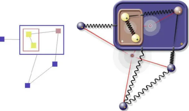
model (right). Grey circle: barycenter, red solid line: gravitational force, zigzag: regular spring force, black solid line: constant spring force [3] . . . 17

LIST OF FIGURES x

2.8 An edge e = {a, b} is connected to its source node a via a port which is located at index 6. The ideal position of node b, ib, is calculated to be right across its port at location 6, an ideal edge length distance away from the port. α is the angle that emerges between the line segment from the port location to ib and the edge e. 20

3.1 An example of node ports in a graph [19] . . . 24 3.2 Different strategies for assigning barycenters [21] . . . 24 3.3 A database schema making use of ports for attribute relationships [22] 25 3.4 A data flow diagram representing a stack [23] . . . 26 3.5 An example of Siebenhaller’s technique of rerouting right and left

side ports to top or bottom [24] . . . 27 3.6 A GeneMANIA gene–gene interaction network automatically laid

out and visualized with Cytoscape.js [4] . . . 28

4.1 A node a is connected to nodes b and c via port constrained edges e and f . With respect to ideal edge length, the edge e is too long in (a) and too short in (b), whereas edge f is too long in both. The horizontal or vertical components of spring forces that are considered as rotational force are indicated. Consequently, the rotational force of node a is|F# »x(e)| −

# » |Fy(f )| in (a) and − # » |Fx(e)| − # » |Fy(f )| in (b) . . . 30 4.2 An example, where a simple edge crossing emerges with

introduc-tion of ports. Even if springs e and f were at ideal edge length, the node repulsion forces between b and c should cause enough tension on the springs causing edge ends to shift. Thereby, the edge crossing should be resolved . . . 31

LIST OF FIGURES xi

4.3 Four different cases of edge end shifting are presented. The blue dashed line indicates the other edge end’s position requirement for edge end shifting. The edge end at port x can shift to port y in (a) and (c), but (b) and (d) fail the location requirement and should not be allowed to do so. . . 32 4.4 An example, where the rotational force of node a does not

ex-ceed the threshold in (a). Performing a 180◦ rotation on node a, however, creates a more stable system (b) . . . 34 4.5 A node a is connected to nodes b and c. The ideal positions of b and

c are ib and ic, respectively. Fb and Fcare the introduced polishing forces pushing nodes b and c to their ideal positions. Forces −Fb and −Fc are also added as reaction pairs. . . 35 4.6 An example where a node a is connected to nodes b, c and d via

Fixed position port constrained edges. Since repulsion and spring forces are stronger than polishing forces, the edge crossing in (a) will not be removed. The proposed heuristic resolves these edge crossings by placing the degree one nodes (b, c and d) directly to their ideal location (b). The node overlaps are eliminated in the later iterations through repulsion. . . 36 4.7 Nodes with ports per side k = 1 (a), k = 3 (b), and k = 5 (c) are

drawn such that corner ports are indicated in red. . . 37 4.8 A simple graph is laid out using CoSEP algorithm while

demon-strating the different phases of the algorithm. Nodes n0, n1, n2 and n3 have Fixed Sided port constraints connecting them to left of node n4. Similarly, nodes n5 and n6 are connecting to node n4 from the right side. Whereas, node n7 should connect to node n4 from top or bottom . . . 40

LIST OF FIGURES xii

5.1 Nodes a, b, c, d, and e are connected to each other via port con-strained edges. Among the nine port concon-strained edge ends, five of them (connected to green ports) are considered properly ori-ented whereas the rest are improper (blue). Thus, the ratio in this layout is %55.56. . . 42 5.2 Number of edge crossings versus number of nodes of our algorithm

(CoSEP) in comparison with CoSE. The percent value denotes the ratio of edge ends with port constraint Fixed Position to the total number of edge ends. In (top-left) %25, (top-right) %50, (bottom-left) %75, (bottom-right) %100 of the edge ends are port constrained. 44 5.3 Ratio of properly oriented edges versus number of nodes of CoSEP

and CoSE. In (top-left) %25, (top-right) %50, (bottom-left) %75, (bottom-right) %100 of the edge ends have Fixed Position port constraint. . . 45 5.4 Number of edge crossings versus number of nodes of our algorithm

(CoSEP) in comparison with CoSE. The percent value denotes the ratio of edge ends with port constraint Fixed Side(s) to the total number of edge ends. In (top-left) %25, (top-right) %50, (bottom-left) %75, (bottom-right) %100 of the edge ends are port constrained. 46 5.5 Ratio of properly oriented edges versus number of nodes of CoSEP

and CoSE. In (top-left) %25, (top-right) %50, (bottom-left) %75, (bottom-right) %100 of the edge ends have Fixed Side(s) port con-straint. . . 47 5.6 Number of edge crossings versus number of nodes of our algorithm

(CoSEP) in comparison with CoSE. The percent value denotes the ratio of edge ends with port constraint either Fixed Position or Fixed Side(s) to the total number of edge ends. In (top-left) %25, (top-right) %50, (bottom-left) %75, (bottom-right) %100 of the edge ends are port constrained. . . 48

LIST OF FIGURES xiii

5.7 Ratio of properly oriented edges versus number of nodes of CoSEP and CoSE. In (top-left) %25, (top-right) %50, (bottom-left) %75, (bottom-right) %100 of the edge ends have either Fixed Position or Fixed Side(s) port constraint. . . 49 5.8 Comparison of the running time of our algorithm (CoSEP) with

CoSE (graph size versus execution time in milliseconds). Edge ends can only have Fixed Position constraint in (top-left), Fixed Side(s) constraint in (top-right), and can have both port constraints in (bottom). . . 50

A.1 A visual scripting graph [5] is laid out with CoSE (a) and CoSEP (b) using Fixed Sided constraints. Respective metrics (CoSE -CoSEP): ratio of properly oriented edge ends: 35.29% - 91.17%, number of edge-edge crossings: 4 - 1, running time 9.65ms - 23.81ms 56 A.2 An SBGN PD map illustrating neuronal muscle signaling is laid

out with CoSE (top) and CoSEP (bottom) using Fixed Sided and Fixed Position constraints. Respective metrics (CoSE - CoSEP): ratio of properly oriented edge ends: 51.35% - 97.29%, number of edge-edge crossings: 4 - 0, running time: 45.04ms - 101.87ms . . . 57 A.3 An SBGN PD map illustrating CaM-CaMK dependent signaling to

nucleus is laid out with CoSE (left) and CoSEP (right) using Fixed Sided and Fixed Position constraints. Respective metrics (CoSE - CoSEP): ratio of properly oriented edge ends: 46.14% - 97.14%, number of edgeedge crossings: 3 0, running time: 31.83ms -73.36ms . . . 58 A.4 An SBGN PD map illustrating insulin-like growth factor (IGF)

signaling is laid out with CoSE (a) and CoSEP (b) using Fixed Sided and Fixed Position constraints. Respective metrics (CoSE - CoSEP): ratio of properly oriented edge ends: 48.27% - 100%, number of edge-edge crossings: 10 - 0, running time 38.7ms - 96.44ms 59

Chapter 1

Introduction

In recent decades, technology has revolutionized our capability to store and re-trieve huge amounts of data. Petabytes of information are processed in just a day. Researching, analyzing and decision making in large scale have become much easier as a result. However, if the information is unorganized or rather indigestible, this can cause confusion and paralysis by analysis. Thus, the main problem nowadays is not about having sufficient data, but rather the struggle has transformed into finding a way to turn raw data into an understandable form.

The concept of visual thinking is a phenomenon in which information can be expressed and understood via virtual processing. Human brains are wired to swiftly interpret and remember visual depictions. In ancient times, humans have carved stone tablets to keep track of finance. Huge chunks of land were surveyed and drawn as maps to guide people. Diagrams are used to explain theoretical models. Everyday we process information in visual form such as logos, charts and drawings. These visual representations are powerful tools that give shapes to abstract concepts making them easier to comprehend. Visualizations can assist in discovering “unstructured” relations or emphasize properties among data entities. Furthermore, utilizing these visual forms have made information visualization a compelling field of study. This field provides techniques in representing abstract data (e.g. numerical or textual description) into intelligible visual form.

(a) Textual representation

(b) Graphical representation

Figure 1.1: Textual vs graph drawing of an example social network

Information visualization consists of unique methods, including cartogram, heatmaping, dendrogram and concept mapping. In this thesis, our focus is on the branch that combines visualization with graph theory named graph drawing. A graph is an abstract structure consisting of objects called nodes and the re-lationship between these objects are called edges. When the data has relational information, graph based visualizations are convenient as the overall structure can be easily mapped to a graph. Thus, graphs are commonly used in many areas. For instance in social networks, people can be represented as nodes and friendship relations between them with edges. This is exemplified in Figure 1.1 where the textual representation of a simple network is drawn as a graph. In biology, protein

production paths and genetic maps can be characterized by graphs. In computer science, a system along with its actors, activities, individual components, and interactions are depicted via Unified Modeling Language diagrams.

The central issue in graph drawing is to situate nodes and edges in such a way that the underlying information is best revealed. Thus, due to human cognition, the limitations to graph drawing come in the form of readability. If the graph drawing area is too large, focusing on the graph may become a problem. Size of the represented graph is also a similar matter. Nodes or edges overlapping one another may confuse the reader. Thus, in order to identify if a graph drawing is “good” or “bad”, there needs to be metrics to evaluate them. There are established aesthetic criteria that quantifies the readability of a graph. Number of edge crossings, number of edge bends, drawing area and maximizing symmetry are some of them.

Graphs can evidently be drawn onto the plane by hand. However, manually placing every object is an incredibly time consuming task [1]. Especially con-sidering the complexity of large graphs. Hence, designing good automatic graph layout algorithms are crucial in building real-time interactive graphical tools for visual analysis.

There has been ample research done on general graph drawing [2] but consider-ably less on compound graph layout [3]. The majority of such work disregard node dimensions (or assume them to be uniform) and neglect specific connection points of edges to nodes. Both of these are common requirements in real life maps (Fig-ure 1.2). Towards this end, this thesis presents a new layout algorithm CoSEP. CoSEP builds on a previous compound spring embedder algorithm named CoSE, adding support for port constraints on edges while respecting non-uniform node dimensions and compound structures in general graphs. The CoSEP algorithm is implemented as an Cytoscape.js extension [4] in an open source library called cytoscape.js-cosep. The algorithm is available online on GitHub.

The following is how the rest of the theis is structured: Chapter 2 presents basic graph theory concepts and graph visualization techniques that are used in

(a)

(b)

Figure 1.2: Part of a visual scripting graph implementing character movement [5] (a) Part of a flow graph used in representing WiFi transmission [6] (b)

this work. Also, information about the CoSE layout algorithm is given. Ports and different types of port constraints are introduced as well. In Chapter 3 we intro-duce layout algorithms that incorporate port constraints in their graph drawings. Also, graph visualization library Cytoscape.js is presented. Chapter 4 explains the novel heuristics developed in CoSEP algorithm in detail. In Chapter 5, we analyze the results of our CoSEP implementation with respect to commonly ac-cepted graph drawing criteria (namely: ratio of properly oriented edge ends and number of edge-edge crossings).

Chapter 2

Background

In this chapter, a summary of the background information regarding the basis of this thesis is presented. Firstly, introductory material about graphs, graph drawing and automated layout algorithms are given. Afterwards, the Compound Spring Embedder (CoSE) algorithm which our algorithm Compound Spring Em-bedder With Support for Ports (CoSEP) is based upon is reviewed in detail. Finally, ports and different types of port constraints are described.

2.1

Graphs

A graph is a mathematical structure that can model relations so that humans can make sense of the underlying data. Depending on the requirements of these systems, graphs can have various properties. Since our work revolves around visualizing graphs, we start with this fundamental structure.

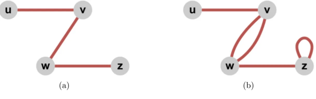
More formally, a graph or a network G = (V, E) consists of two sets, where V is the set of nodes (vertices) and E is the set of distinct pairs called edges. An edge e = {u, v} is the relationship between nodes u and v, where u, v ∈ V . These nodes u and v, are called the endpoints of edge e. For example, Figure 2.1(a) depicts a simple graph where V = {u, v, w, z} and E = {{u, v}, {v, w}, {w, z}}.

A pair of distinct nodes u and v are said to be adjacent if they are connected by an edge e = {u, v}. Also, nodes u and v are incident to edge e. Likewise, a pair of distinct edges e and f are adjacent if they have a common endpoint.

If an edge starts and ends at the same node, then that edge is called a self-loop. Furthermore, there can be more than one edge connecting between a pair of nodes referred to as multi-edges. Figure 2.1(b) illustrates these concepts where node z contains a self-loop, and nodes v & w are connected by two edges. A simple graph does not contain any self-loops or multi-edges.

(a) (b)

Figure 2.1: Some sample small graphs

Edges in a graph may represent a sense of direction. In that case, node pairs that have an edge between them are considered ordered. If all node pairs in a graph G are ordered, then graph G is a directed graph. On the other hand, if all node pairs are unordered, then graph G is a undirected graph.

The number of edges incident to a node u is called the degree of node u. When the graph is directed, the total number of incident edges of a node u, where node u is the target endpoint is the indegree of node u. Likewise, the outdegree of a node u is the total number of incident edges that have node u as their source endpoint.

A subgraph G0 = (V0, E0) of a graph G is a graph, where each node in V0 belongs to V and each edge in E0 belongs to E. Subgraphs of a graph can be obtained by removing edges and/or nodes from said graph.

A simple path is a path with non-repeating nodes. A circuit is a path that starts and ends at the same node. A cycle is a circuit in which all nodes are distinct except for the starting and ending nodes. A graph with no cycles is an acyclic graph. A graph is connected if any two nodes are connected by a path. Otherwise, the graph is called disconnected.

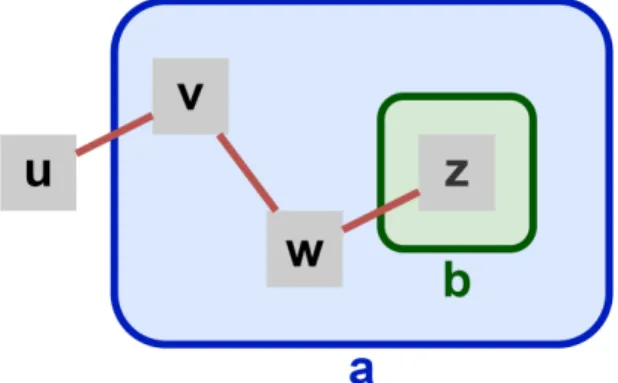
A tree is a graph in which all pair of nodes are connected by a single path. A forest is a disconnected graph where each component is a tree. In a rooted tree, one particular node is distinguished as the root. A node u is an ancestor (descendant) or parent (child) of node v if u lies in the path to (from) the root node from (to) v. The root has no parent and every other node is its descendant. A compound graph C = (V, E, F ) contains a set of nodes V , a set of adjacency edges E, and a set of inclusion edges F [3]. The inclusion graph T = (V, F ) is a rooted tree, defined on nodes V and inclusion edges F . However, no adjacency edge may connect a node to one of its descendants or ancestors. An example is given in Figure 2.2, where V = {u, v, w, z, a, b}, E = {{u, v}, {v, w}, {w, z}} and F = {(a, v), (a, w), (a, b), (b, z)}. Nodes a and b are both compound nodes. Moreover, node b is parent node of z, but a child node of a.

2.2

Graph Visualization

A drawing or layout of a graph is the visual representation of the graph’s math-ematical structure. Graphs can be displayed in a 2D plane or 3D space. Yet, 2D graph drawings where graphs are drawn as node-link diagrams are more frequently used in exploring data. In general, nodes are represented by simple shapes (e.g. point, rectangle, circle) and edges as straight or curved edges. Directed edges can be indicated with arrows at edge ends. Visual elements of the graph are also crucial in increasing the comprehension level of the underlying graph data. Thickness of the edge lines, opacity of the edges or nodes, dimensions and colors of the nodes are some of the examples that are important in graph visualiza-tion. Ultimately, research in graph drawing focuses on both designing automated layout algorithms and real-time interactive graphical tools.

Layout algorithms calculate the positions of nodes and edges on a 2D plane in order to make the graph most visually appealing. Even with simple graphs, positions of the graph objects is vital in creating readable drawings. Figure 2.3 shows an example of a graph being laid out by two different layout algorithms. The layout algorithm in Figure 2.3(a) is much simple and easy to compute al-gorithm. Nevertheless, the algorithm fails to properly display the edge (v1, v7) as it overlaps edges (v1, v4) and (v4, v7). Thus, the circular AVSDF algorithm in Figure 2.3(b) requiring additional execution time can be justified in this case. Considering the complexity of real life systems, layout algorithms can often be application dependent. A new complex system that is modelled by a graph can call for a different graph structure or a different set of layout requirements. In that case, a new layout algorithm is designed to tackle these additional problems. Di Battista et al. [2] proclaims that there are three fundamental concepts defin-ing the layout requirements for a “nice” drawdefin-ing. These concepts are drawdefin-ing conventions, drawing aesthetics and drawing constraints. Drawing conventions are the commonplace rules which must be fulfilled. For instance, straight line drawings represent each edge as a straight line segment whereas orthogonal draw-ings represent them as a chain of horizontal and vertical line segments. Drawing

(a) (b)

Figure 2.3: A grid layout (a) and a circular AVSDF [7] layout (b) performed on the same graph

aesthetics are visual criteria that measures the comprehensibility aspect of the drawing. Although these criteria can be subjective, many standards have been put in place by performing empirical studies regarding the human understanding of drawn graphs [8]. Some of the accepted common criteria are [2]:

• Minimize the number of edge crossings • Minimize drawing area

• Minimize node overlaps • Maximize symmetry • Uniform edge length

Selecting a set of aesthetic criteria is often an application dependent process as some of them are contradictory in nature. Sometimes, a certain criterion takes precedence over others as it best defines the quality of the drawing. Lastly, drawing constraints are additional rules imposed on a subgraph rather than the whole graph. For example, forcing a particular node to be left of another certain node or forcing a specific node to be at the center of the drawing.

Usually, one can not effectively analyze data by looking at a static image of a graph. In order to overcome this issue, graphical tools add the ability to interact with the graph. Thus, interaction and navigation techniques are used together with layout algorithms in graph visualization tools. Examples of interaction in-clude the capability to alter graph topology by adding / removing graph objects, moving nodes around the canvas, and highlighting specific graph objects. A com-prehensive overview can be found in [9]. As for large networks, its complexity has to be dealt with so as to not confuse the user. Complexity management tech-niques range from simple rendering methods like panning, zooming and ghosting, to collapsing the compound nodes of a hierarchical network, to temporarily hiding unwanted parts of the topology [10].

2.3

Automated Layout Algorithms

The past two decades have seen a fast growing body of research dedicated to designing algorithms to construct aesthetically pleasing drawings of graphs [2]. There are numerous layout algorithms in the literature under various categories. However, only two types of layout algorithms, namely force-directed layout and Sugiyama’s framework [11] are relevant to this work. The underlying physical model of both CoSE and CoSEP algorithm is an altered force-directed model (see Section 2.4 for details). On the other hand, the related methods which have different forms of port constraints are all orthogonal drawings utilizing Sugiyama’s framework.

2.3.1

Force-directed Algorithms

Force-directed layout algorithms (aka spring embedders) are arguably the most popular approach to automatic graph layout. One of the pioneers of the force-directed model is the Eades algorithm [12]. Eades is the first one to introduce physical forces of attraction and repulsion. The basic idea is to simulate a phys-ical system in which nodes behave as electrphys-ically charged metal rings, and edges

represented by physical springs of a specified ideal length. Springs exert forces to their connected objects proportional to the deviation from their “natural” length. Instead of following Hooke’s law, Eades uses his devised logarithmic springs for the attraction force. In order to avoid node-to-node overlaps, nodes in the graph repel each other. The equations for the attraction (spring) and repulsion forces are the following [13]:

fspring(pu, pv) = cσ · log kpu− pvk l · # »pupv (2.1) frepulsion(pu, pv) = c% kpu − pvk2 · # »pupv (2.2)

where nodes u, v ∈ V , vectors pu = (xu, yu) and pv = (xv, yv) are of node positions, cσ and c%are constants decided empirically, and l is the natural length of a spring. The layout algorithm simulates this underlying physical model by moving en-tities corresponding to nodes iteratively with respect to total forces acting upon them, until the system of entities reach a relatively stable state, in which the overall energy is minimal. Eades focuses on graphs with up to 30 nodes and pro-claims that “Almost all graphs reach a minimal energy state after the simulation step is run 100 times” [12]. Thus, time complexity of the Eades algorithm is O(|V |2_{+ |E|)). However, notice that today’s graphs are much larger than those} at the time. Hence, the number of steps required typically go a lot more than a 100 with today’s real-life graphs.

Figure 2.4 illustrates a force-directed algorithm’s physical modeling of a undi-rected graph. The physical model is “let go”, and the movement of the nodes are simulated. After reaching an equilibrium state, the model can be reverted and the corresponding graph can be drawn.

Fruchterman and Reingold (FR) presents an improved version of the Eades algorithm [14]. Similar to the Eades algorithm, FR treats nodes as “atomic particles or celestial bodies” that repel one another and adjacent nodes attract

Figure 2.4: A physical analogy of the force-directed algorithms [13]

each other via springs. Furthermore, FR algorithm aims to distribute nodes evenly across the entire drawing area. The equations for the attraction (spring) and repulsion forces that resemble Hooke’s law are as follows [14]:

fspring(pu, pv) = d2 k (2.3) frepulsion(pu, pv) = − k2 d (2.4)

where d is the distance between two nodes and k is a constant representing the optimal distance between nodes. k can be calculated as:

k = C ·r area

|V | (2.5)

where constant C is found experimentally and area is the size of the drawing area.

In addition to the force scheme, FR introduces the concepts of temperature and cooling. Temperature is a concept that directly limits the movement of nodes. The idea is that layout starts with a high temperature value, and as nodes move around, temperature of the system cools down. In other words, as the layout starts to stabilize, adjustments made to the nodes gets smaller. This is done to prevent excessive node movements that can happen when the system is close to an equilibrium. Moreover, nodes have a maximum amount of distance they can move in each iteration, also limiting any drastic movement.

FR’s basic algorithm still has the same time complexity as the Eades algorithm. In each iteration, calculations of spring forces take O(|E|) time and repulsion forces take O(|V |2) time. Thus, FR focuses on reducing the time complexity of repulsion force calculations. The observation FR makes is that node pairs that are far way from one another produce repulsion forces that are negligible. In order to remove such calculations, FR presents the grid-variant algorithm. In this algorithm, the drawing area is divided into a grid of squares in each iteration. Every vertex belongs to a particular grid depending on its position on the canvas. A node considers repelling only the nodes that are placed in the same grid or the neighboring grids. For instance in Figure 2.5, node v can repel only node q as node s is considered but rejected for being too far away, and node r is not in a neighboring grid. Therefore, the time complexity mentioned above can be asymptotically reduced to O(|E| + |V |). Similar to Eades, FR focuses on graphs with up to 40 nodes and simulation is run for 50 iterations but recent experiments show that the algorithm scales fairly well for small to medium sized graphs (up to several thousands nodes).

Figure 2.5: Calculating repulsion forces using the grid-variant [14]

Due to directed algorithms’ simple design, there are numerous force-directed algorithms published in recent decades. The force model approach is utilized in many applications like visualizing clustered graphs [15] and biological process description maps [16]. A detailed survey analyzing different adaptations of the force-directed algorithm can be found in [17].

2.3.2

Sugiyama Framework

The most popular graph drawing method on directed graphs is the layered ap-proach introduced by Sugiyama et al [11]. Sugiyama’s framework is supported by almost all graph drawing libraries. This approach places nodes in a series of layers or hierarchies such that almost all edges point in the same direction. The classic Sugiyama algorithm’s orientation is top-to-bottom, so layers are aligned horizontally. The algorithm has five steps as follows (Figure 2.6):

• Removing Cycles: In order to make sure that the majority of the edges point towards the same direction, cycles of the graph are temporarily eliminated by reversing minimal subset of edges.

Figure 2.6: A directed graph drawn according to the Sugiyama framework [18] with polyline edge routing

• Layer Assignment: Nodes of the graph are assigned to subsequent horizontal layers. A feasible assignment is one where all edges have correct orientation. Furthermore, edges should only connect to nodes on adjacent layers. If that’s not the case and edges span more than one layer, such edges are replaced by a series of connected dummy nodes and edges to ensure this. • Crossing Reduction: Edge crossings between layers are removed by

rear-ranging the nodes in each layer. Sugiyama proposes a method for this reordering called the barrycenter heuristic. This heuristic is simply based on placing a node at the average of the x-coordinates of its neighbors. It only considers two layers at a time where one layer is fixed and the other layer is reordered. In order to reorder every layers, the layer sweep algo-rithm crosses pairs of adjacent layers repeatedly until no edge crossings can be removed further.

• Horizontal Coordinate Assignment: Nodes in each layer are given x-coordinates such that edges are drawn as straight as possible.

• Edge Routing: The added dummy nodes are omitted, edges that were re-versed are restored and edge bends are added to the graph. The positioning of the edge bends are decided depending on whether the drawing is polyline or orthogonal.

2.4

Compound Spring Embedder (CoSE)

The CoSE algorithm is based on the Fruchterman and Reingold’s (FR) grid-variant algorithm introduced in Section 2.3.1. The force-directed approach is improved upon to have support for non-uniform node sizes, compound nodes, arbitrary level of nesting and inter-graph edges [3]. Similar to FR, the idea is to simulate a physical system obeying the laws of Newton, Hooke and Coulomb, in which nodes behave as electrically charged physical entities, and edges represented by physical springs of a specified ideal length.

Figure 2.7: A sample compound graph (left), and the corresponding physical model (right). Grey circle: barycenter, red solid line: gravitational force, zigzag: regular spring force, black solid line: constant spring force [3]

Compound nodes are handled by representing an expanded node and its asso-ciated nested graph as a single entity, similar to a “cart”, which can move freely in orthogonal directions [3]. A compound node can have child compound nodes represented as carts stacked on top of each other (Figure 2.7). There is no limit to the number of nested compound nodes. Moreover, compound nodes adjust their node dimensions in each iteration as the child nodes move around.

The force-directed algorithms presented in Section 2.3.1, assume that all nodes have identical node dimensions. So, they simplify the spring concept. All springs have the same ideal length and their length calculation is from node center to node center. This simplified approach does not work when node dimensions are different or when there are compound nodes. Thus, CoSE defines edge length to be the line segment going through one end node’s center to the other, clipped on both sides by the rectangles representing the end nodes (see equation 2.6). Edges that span across compound nodes have different ideal lengths than normal edges. This difference depends on the number of nesting structures it spans across.

Repulsion forces are calculated similar to the FR’s grid-variant. Only neigh-boring nodes that are “too close” repel each other. Evidently, compound nodes do not repel their child nodes. In order to simplify calculations, repulsion forces only apply to nodes that are in the same graph. If for some reason nodes over-lap, the repulsion force between the overlapping nodes are increased substantially depending on the overlapping area.

The spring and repulsion forces are calculated as follows [3]:

fspring(pu, pv) = (λ − kpu− pvk)2 η # » pupv (2.6) frepulsion(pu, pv) = α kpu− pvk2 # » pupv (2.7)

where vectors pu = (xu, yu) and pv = (xv, yv) are of node positions, λ is the ideal edge length, η is the elasticity constant of the edge, and α is the repulsion constant.

In addition to spring and repulsion forces, CoSE introduces gravitational forces that keep graph components together. This force is relatively minor compared to other forces. Its magnitude does not depend on node dimensions or the distance between node and gravitation center. When the graph is disconnected, gravi-tational forces move disconnected components towards the center of the graph. Also, each compound node has gravitational forces that keeps its child nodes closer to the center. This force has a great affect in keeping the overall drawing area small.

In Section 2.3.1, both force-directed algorithms placed nodes randomly across the canvas at the start of the layout. In contrast, CoSE algorithm has a incre-mental layout option. If this option is picked, the current positions of the nodes are respected and the layout algorithm starts from here. Otherwise, nodes are distributed randomly or radially, depending on whether the graph is a forest and flat.

Algorithm 1 The CoSE Algorithm [3]

1: _{Initialize(C)} 2: totalIter ← 0

3: if layoutT ype 6= incremental then

4: if graph is f orest and f lat then

5: _{PositionNodesRadially(C)}

6: else

7: _{PositionNodesRandomly(C)}

8: end if

9: end if

10: while totalIter < maxIterations do

11: totalIter ← totIter + 1

12: if totIter % convP eriod = 0 then

13: _{if converged() then} 14: break 15: else 16: _{UpdateCoolingFactor()} 17: end if 18: end if

19: _{UpdateBounds(C)} . resize compounds

20: _{CalcSpringForces()} 21: _{CalcRepulsionForces()} 22: _{CalcGravitationalForces()}

23: _MoveNodes() . w.r.t. total forces

24: end while

During the layout algorithm, each node moves according to the total force of spring, repulsion and gravitation forces acting upon it. For compound nodes, the forces inflicted are propagated among their child nodes. There is also a maximum limit on the movement of each node so that there are no drastic movements. The temperature is periodically cooled down similar to the FR algorithm. The layout stops when the total movement of nodes drops below a threshold value indicating that the graph is in a relatively stable state. At this point, the layout is said to converge. The main algorithm implementing the heuristics mentioned in this section can be found in Algorithm 1.

Spring forces are calculated for each edge, whereas repulsive forces are calcu-lated for each node pair, and gravitational forces are calcucalcu-lated for each node. Thus, the run time complexity of one iteration in CoSE algorithm is O(|V |2_+|E|),

where the dominating term is from the node repulsion calculation as distances between all node pairs are checked. In the worst case, like the FR algorithm, the overall complexity of the layout becomes O(|V |3 _{+ |E| · |V |). However, with the} grid-variant adapted from FR, it can be reduced to O(|V |2 _{+ |E|).}

2.5

Port Constraints

In this work, we assume that we are dealing with nodes that have rectangular geometry. Ports or connection points are realized as discrete points along the edges of the associated rectangle, an equal number on each side (see Figure 2.8). A node having ports can be imagined as a logic gate or a micro controller with a pre-configured port interface. The ports then can be indexed clock-wise as {0, 1, 2, . . . , 4k − 1} starting at the top-left where k > 0 is the number of ports on each side, specified by the user. The incident edge endpoints of this node must connect to these particular connection points.

The port constraints are mainly associated with edge ends. When an edge end does not have a specified port constraint, it’s assumed that it connects to their end nodes at their center, usually shown as clipped at the intersection point of the line segment representing the edge and the rectangle representing the node.

Figure 2.8: An edge e = {a, b} is connected to its source node a via a port which is located at index 6. The ideal position of node b, ib, is calculated to be right across its port at location 6, an ideal edge length distance away from the port. α is the angle that emerges between the line segment from the port location to ib and the edge e.

We further assume that any node, including compound nodes and those nested inside compound ones, is allowed to have port constraints defined on its incident edges. An edge may have a possibly different port constraint on each end, chosen from the following types:

• Free: The specified end of the edge can be placed at any port of the associated node. For instance, source of edge e in Figure 2.8 can be defined as “free”, implying it may be connected to node a at any one of the 20 ports available in a.

• Fixed Side(s): A set S of directions is assigned to each end of an edge: S = {s | s ∈ {top, lef t, bottom, right}}. The specified end of the edge can be assigned to any port on one of these sides. For instance, if source of edge e in Figure 2.8 is defined to have “fixed sides” of {right, lef t}, then the edge will only be allowed to be connected to a at ports 5 through 9 or 15 through 19.

• Fixed Position: The specified end of the edge is assigned to a fixed port of the associated node. For instance, if edge {a, b} in Figure 2.8 is to have a fixed port constraint of 6 on its source, then the only valid assignment of this end of the edge is as shown in this figure.

For each port we define an ideal position (defined by the user in line with their particular domain / application), a point in the canvas right across the port. This location is one ideal edge length away from the corresponding port. Consequently, an angle is formed between the edge and the line ray emanating from the port and going towards the ideal location. These concepts are important as they show the deviation from “ideal” placement. For instance in Figure 2.8, the edge e would have intersected node a if angle α was an obtuse angle. Therefore, these angles and ideal location of ports are essential in CoSEP’s heuristics.

The absolute value of α in Figure 2.8 can be found using the vectorsp# »6ib (port p in node a at index 6 to the ideal position ib of node b) and

# »

p6b (port p at index 6 to the center of node b). If the edge end of e incident to node b was

also positioned on a port, then vector p# »6b would have pointed towards this port instead. Subsequently, α can be calculated as:

kαk = arccos # » p6ib·p# »6b # » p6ib · # » p6b (2.8)

Note that most of the heuristics introduced in Section 4 requires only the absolute value of the angle. For others, the location of vector p# »6b relative to vector p# »6ib is important. We indicate this by using signed angle values. A angle is positive if vectorp# »6b is right (clockwise) ofp# »6ib and negative if vice-versa. This positioning can be found as follows:

# » p6b = (ux, uy) # » p6ib = (vx, vy) λ = uxvy− uyvx (2.9)

if λ is positive then vectorp# »6b is to the left of vectorp# »6ib, otherwise if λ is negative then vectorp# »6b is to the right.

Chapter 3

Related Methods and Libraries

In this section, various graph drawing algorithms with support for ports are introduced. Each layout algorithm approaches to the problem of port constraints differently since the concept of a port is defined according to the underlying domain and graph model. Almost all of the related algorithms use the Sugiyama framework (see Section 2.3.2 for more details). Finally, at the end of this chapter, the graph visualization library Cytoscape.js is presented.

3.1

Related Methods

Numerous graph drawing algorithms have been proposed to visualize port con-strained graph models such as data structure maps, data flow diagrams, schemat-ics of digital circuits and biochemical networks. Gansner et al. [19] introduces the concept of “node ports” in their novel technique of drawing directed graphs. They show how node positioning can be modified so that coordinate offsets from node ports are handled (Figure 3.1). Sander [20] presents a layout algorithm for drawing data structures using the Sugiyama framework for the VCG tool. The problem of side ports are handled by adding dummy nodes and later routing edges through these dummy nodes. On the other hand, Waddle [21] is the first to

Figure 3.1: An example of node ports in a graph [19]

propose altering the barycenter heuristic done during cross minimization in order to handle the port problem of data structures. Figure 3.2 illustrates various ways of modifying the barycenters.

(a) To node center (b) To edge end

(c) To node center (d) Secondary barycenters

(e) Alternate scheme

Figure 3.2: Different strategies for assigning barycenters [21]

Due to the nature of data structures, these works mentioned above do not support multiple types of port constraints. An added port constraint can only restrict an edge endpoint to a fixed position around a node. With techniques such as spline curve edge routing, rotating nodes, barycenter heuristic and dummy

Figure 3.3: A database schema making use of ports for attribute relationships [22]

nodes, these fixed edge endpoints are integrated into the layer-based approach, especially suitable for directed graphs.

Battista et al. [22] describe a way to draw database schemas in which database tables are depicted as rectangular boxes consisting of table attributes. Edges, called links, connect two different table attributes together representing referen-tial constraints or join relationships. These edges can connect to their respective attributes only from the right or left side of the associated table row (Figure 3.3), which is a good example of a rather special type of a domain-specific port con-straint.

The series of published work by Schulze et al. [23] are specifically for visu-alizing data flow diagrams, also using the layer-based approach. They develop several extensions to the barycenter heuristic to support port constraints. They have defined five different levels of port constraints to cover the requirements of data flow diagrams (Figure 3.4). The level of a port constraint indicates the hier-archical level from “flexible” to “restrictive”. These port constraints in order are: Free, FixedSide, FixedOrder, FixedRatio, and FixedPosition. Therefore, the main

Figure 3.4: A data flow diagram representing a stack [23]

algorithm, which has five phases, transitions port constraints down this hierarchy in each phase. In the end, each port constraint is reduced to a definitive position relative to its node. The algorithm produces needless edge-edge crossings of inter-hierarchy edges as they layout compound graphs in a naive, bottom-up manner (i.e., processing the most nested actor diagrams first) [23]. The overall solution is focused on the nature of data flow diagrams, where nodes are hierarchical and the main orientation of edges are left to right (or top to bottom).

Siebenhaller [24] defines port constraints in orthogonal graph drawing with more flexibility. Similar to our approach, ports are distributed evenly around the node, constraints are associated with edges and not every edge has to be port constrained. In order to reduce edge crossings during crossing reduction step, they further transform the problem to a minimum cost flow network. As depicted in Figure 3.5, they reroute a node’s right and left side ports locally to top or bottom with an edge bend. The algorithm is shown to work on UML activity diagrams.

The graph drawing algorithms presented in this section center around visu-alizing simple graphs with edges routed orthogonally. On the other hand, the CoSEP algorithm proposes a novel approach to draw port constrained compound graphs with straight line drawings and non-uniform node dimensions. With the help of our coverage for varying port constraints, our algorithm is applicable to most domains. Since CoSEP differs too much from previous related work as the main objectives are dissimilar, its performance is compared with its predecessor in Section 5, CoSE algorithm.

Figure 3.5: An example of Siebenhaller’s technique of rerouting right and left side ports to top or bottom [24]

3.2

Cytoscape.js

Cytoscape.js is an open-source JavaScript-based graph library that provides a JS application programming interface (API) to enable software developers to inte-grate graphs into their data models and web user interfaces [4]. The API supports drawing and editing undirected / directed compound graphs. The graph elements can be interactively added and removed. Various graph drawing algorithms like grid layout, circular layout, concentric layout, breadth-first layout, and CoSE lay-out are available (Figure 3.6). Several well-known graph theory algorithms—such as connectivity search, shortest path, minimum spanning tree, minimum cut, ranking and centrality measures—are included [4]. The API provides a variety of styling options for graph elements. Labels, different types of edges / nodes, different edge arrow types, coloring and opacity of graph elements are some of the customization options. Interactive functions are also included in the API. The viewport can be zoomed or panned, graph elements can be selected and dragged. Animations can be used to increase the salience of particular elements in the graph and to provide visual continuity to the user when programmatic changes to the graph are made [4].

Cytoscape.js API allows developers to build extensions on top of the core li-brary. For instance, cytoscape.js-expand-collapse extension provides an in-terface to expand / collapse nodes and edges for better management of complexity

Figure 3.6: A GeneMANIA gene–gene interaction network automatically laid out and visualized with Cytoscape.js [4]

of compound graphs [10]. The cytoscape-cose-bilkent extension implements the CoSE algorithm explained in Section 2.4. The CoSEP algorithm is also im-plemented as an extension called cytoscape.js-cosep.

The visualizations in this thesis are mostly produced using the Cytoscape.js library.

Chapter 4

CoSEP Layout Algorithm

In this chapter, we present the new heuristics and force types that were added on top of the CoSE layout structure in detail. All of the following sections apart from the last one, explain an addition that was made to the basic model. The final section explains the flow of the main algorithm and how the heuristics were integrated to the overall structure.

4.1

Underlying Physical Model

The CoSEP algorithm is a basic force-directed layout that employs spring, repul-sion and gravitation forces from the CoSE algorithm. In fact, everything that was presented about the CoSE algorithm in Section 2.4 also applies to the CoSEP algorithm. However, the spring calculation method from CoSE is modified to consider ports. If an edge does not have a port constraint on both its edge end-points, the calculation is still the same. In that case, the edge is a line segment that connects to the center of both source and target node, clipped with respect to their node dimensions. However, if an edge endpoint is port constrained, the line segment ends at the associated port location (without being clipped).

(a) (b)

Figure 4.1: A node a is connected to nodes b and c via port constrained edges e and f . With respect to ideal edge length, the edge e is too long in (a) and too short in (b), whereas edge f is too long in both. The horizontal or vertical components of spring forces that are considered as rotational force are indicated. Consequently, the rotational force of node a is|F# »x(e)| −

# » |Fy(f )| in (a) and − # » |Fx(e)| − # » |Fy(f )| in (b)

called rotational forces. This force does not move nodes around like the forces presented before. It is used purely to measure the state of the nodes and edge ends. The heuristics makes decisions according to the direction and magnitude of rotational forces (to be detailed in the section on the relevant heuristic). This force is actually the rotational component of a spring force that emerges because of an edge. In other words, we take the horizontal or vertical component of the exerted spring force depending on which node side the port is located at and whether the spring is pulling or pushing. The sign of this force is positive if its direction around the node is clockwise, and negative otherwise. The rotational force of a node is the sum of all the incident edge endpoints’ rotational forces. Figure 4.1 gives an example from a graph with two different states.

4.2

Shifting Edge Endpoints

A node can connect to many other nodes without any problem in the CoSE algorithm. However, since ports are defined in a discrete manner, introduction of port constraints can easily introduce edge to edge crossings in the drawing. While not much can be done for edge ends with Fixed Position constraints, edge ends

Figure 4.2: An example, where a simple edge crossing emerges with introduction of ports. Even if springs e and f were at ideal edge length, the node repulsion forces between b and c should cause enough tension on the springs causing edge ends to shift. Thereby, the edge crossing should be resolved

with Free and Fixed Side port constraints can be re-arranged to reduce such edge crossings (Figure 4.2). Thus, we introduce the ability for edge ends to shift from port to port. There is no limitation to the amount of incident edge ends a port can have. So, edge ends should be able to freely shift as the layout progresses, and yield a better graph drawing.

Edge end shifting is decided using rotational forces described in the previous section. An edge end is considered for a shift depending on the direction and magnitude of the related force. If the magnitude is bigger than a pre-defined, empirically determined, threshold, then the edge end is shifted towards the ro-tational force’s direction. Instead of shifting edge ends at every iteration, it is applied once in every fixed number of iterations in order to prevent possible os-cillations. Thus, the rotational forces are averaged over this fixed number of iterations.

Edge ends with Free port constraints can potentially shift to any one of the ports around a node. On the other hand, Fixed Sided port constrained edge ends can only shift to ports that are on the allowed node sides. But, this allowed range is not circular. Meaning, edge ends can not jump over node sides. They can only change node sides if they are directly adjacent to it. Nevertheless, we have noticed that some Fixed Sided port constraints like {top, bottom} or {right, left} are actually common in certain domains. For such port constrained edge ends, they are allowed to jump to the port at the opposite node side.

been added to edge ends that wish to change node sides. This is done on top of the rotational force threshold. The other edge end of the edge (center of the incident node if unconstrained), has to be in an acceptable relative position. This respective location is based on a diagonal line that goes through the center of the node and the corner of the node residing between associated sides. In cases where an edge end considers jumping to the opposite node side, the mentioned line goes through the center of the node, and is parallel to the two sides of the node. These cases are depicted in Figure 4.3.

(a) (b)

(c) (d)

Figure 4.3: Four different cases of edge end shifting are presented. The blue dashed line indicates the other edge end’s position requirement for edge end shifting. The edge end at port x can shift to port y in (a) and (c), but (b) and (d) fail the location requirement and should not be allowed to do so.

4.3

Rotating Nodes

When port constraints are too restrictive (i.e., there are too many Fixed Position or strict Fixed Sided port constraints), the initial layout of the graph becomes especially important. Since the system is fairly limited, shifting edge ends heuris-tic either fails to resolve edge crossings or the slow shifting becomes a bottleneck on the algorithm’s run time. On the other hand, the user might define port con-straints according to a particular node orientation. Certain domains only care about the relative positioning of the edge ends, and there is no restriction on the node orientation. Thus, we introduce the ability for nodes to rotate. An option is given to the user per node to decide so they can turn the rotation off for certain nodes or globally.

The rotational forces described in Section 4.1 is also utilized for this heuristic. The reason for using rotational forces is that incident port constrained edge ends can repeatedly pull or push the node towards a certain direction. If this force is consistent over a period of iterations, then there is local instability in the system. Rotating the node 90◦ accordingly can make the system more stable.

In certain instances, the rotational forces are not enough to detect a needed rotation (Figure 4.4). In such cases, rotating the node 180◦ would be more appro-priate. Thus, we defined two types of 180◦ rotations: top-bottom and left-right. In fact, it can be defined more as a swap operation between opposite node sides. For instance in a top-bottom rotation, the edge ends on the top are shifted to bottom with respect to port index ordering, and vice-versa. But, the ports on left and right node sides are left intact. A 180◦ node rotation can be determined by checking if the majority of incident edges have obtuse angles. Evidently, top-bottom and left-right rotations are checked separately. Edges that are connected to degree one nodes are to be handled separately. Hence, they are not taken into account in the mentioned heuristic.

When a node rotation, either 90◦ or 180◦, occurs, edge end port constraints are modified to accommodate for these new changes. For instance, a Fixed Sided edge

(a) (b)

Figure 4.4: An example, where the rotational force of node a does not exceed the threshold in (a). Performing a 180◦ rotation on node a, however, creates a more stable system (b)

end with {top, bottom} port constraint, will turn into {right, left} port constraint after a 90◦ clockwise rotation, and back into {top, bottom} port constraint after another clockwise rotation. Thus, we intend for this heuristic to be intertwined with edge end shifting heuristic. One should take place after the other. Since rotation of nodes is a heuristic chancing the drawing more drastically, it should be applied less frequently than others. However, node rotation is given priority when two heuristic periods coincide.

4.4

Moving Nodes to Their Ideal Positions

In order to provide an aesthetically pleasing graph drawing, we believe that nodes should be near, if not exactly at, their ideal positions (as defined in Section 4.1). Thus, we present another kind of force called polishing force for this purpose (Figure 4.5). Here in order to comply with Newton’s third law (i.e., forces always come in action-reaction pairs with equal magnitude in opposite directions), we add a reaction force to the other end node with the associated port as well. Notice, however, that polishing forces only apply to edges with exactly one edge end being port constrained.

Figure 4.5: A node a is connected to nodes b and c. The ideal positions of b and c are ib and ic, respectively. Fb and Fc are the introduced polishing forces pushing nodes b and c to their ideal positions. Forces −Fb and −Fc are also added as reaction pairs.

Polishing forces are calculated similarly to the gravitational forces. The di-rection of the force is orthogonal to the edge and towards the ideal location. Its magnitude is calculated to be the distance (to the ideal position) times some constant decided empirically. Similar to gravitational forces, these forces are comparatively weaker than spring and repulsion forces.

4.5

Further Handling of Degree One Nodes

Generally, the polishing forces specified above are adequate on their own to min-imize edge crossings. But polishing forces struggle to minmin-imize edge crossings when port restrictions are too strict or when a node is incident to too many edges. For cases such as the one in Figure 4.6, the spring and repulsive forces result in a standstill and can not be resolved by polishing forces. Therefore, we introduce a procedure that places one degree nodes directly at their ideal position. Like the previous heuristics described above, this heuristic is also done periodi-cally. Although it is a drastic action, we do this to ensure that the neighboring

(a) (b)

Figure 4.6: An example where a node a is connected to nodes b, c and d via Fixed position port constrained edges. Since repulsion and spring forces are stronger than polishing forces, the edge crossing in (a) will not be removed. The proposed heuristic resolves these edge crossings by placing the degree one nodes (b, c and d) directly to their ideal location (b). The node overlaps are eliminated in the later iterations through repulsion.

nodes scatter and do not reverse the improvement done by this heuristic.

4.6

Algorithm

The new algorithm expands the CoSE algorithm to five phases, including the initialization stage, in order to better incorporate port constraints. Three of these stages (Phase II , III and IV) involve the recently presented heuristic techniques. Hence, the major steps of CoSEP are as follows:

• Initialization: The necessary arrangements such as for the CoSE algorithm are done in this phase. Structures for a compound graph manager are constructed. Threshold for convergence and ideal edge lengths for inter-graph edges are calculated. Assuming incremental option is not chosen, nodes are distributed randomly across the drawing area. Otherwise, the algorithm skips to Phase II.

• Phase I: The initial positions of nodes are rather important for the success of the CoSEP algorithm. Thus, we use the CoSE algorithm with reduced

number of iterations to construct us a starting graph drawing. CoSE al-gorithm has a “draft” layout option which has a relatively faster cooling schedule. This gives CoSEP a nice “rough” drawing which can reach a stable state much easier than a randomly laid out graph.

• Phase II (initializing ports): Port constraints are realized in this phase. Evidently, Fixed Position port constrained edge ends are easily assigned to their pre-defined ports. As for others, they are assigned to “corner ports” that are closest to the other end node’s center. Corner ports are ports that are directly adjacent to a node corner (Figure 4.7). Note that for Fixed Sided port constraints, the corner ports have to be valid (i.e., in line with the constraints).

• Phase III: The spring embedder starts again with a lower cooling factor. Rotational forces and angles of edge endpoints, necessary for various heuris-tics, are calculated together with spring, repulsion and gravity forces. The heuristic procedures of shifting endpoints, rotating nodes and handling de-gree one nodes are performed in this phase.

• Phase IV (polishing phase): This phase is considered as the polishing phase. In contrast to Phase III, only the heuristics related to handling of degree one nodes are applied. Furthermore, initial cooling factor is even lower than Phase III as this phase is expected to minimally alter the previously established layout.

(a) (b) (c)

Figure 4.7: Nodes with ports per side k = 1 (a), k = 3 (b), and k = 5 (c) are drawn such that corner ports are indicated in red.

The CoSEP algorithm described above can be integrated to CoSE’s main method in Algorithm 1 by extending it as presented in Algorithm 2. The visual-ization of the CoSE algorithm using a simple graph can be found in Figure 4.8. The important thing to consider is that heuristics mentioned in this chapter are distributed to phases described above. Each heuristic and the convergence check is performed at certain periods instead of every iteration. The length of these periods are unique parameters that were determined empirically.

The main and only goal of Phase II is to realize ports and port constraints on the compound graph structure C. On the other hand, phases following Phase II all have a separate spring embedder that calculates forces, move nodes with respect to the compound node structure, and implement the relevant heuristics. Thereby, the necessary parameters such as the cooling schedule are initialized before the respective phase.

Algorithm 2 The CoSEP Algorithm 1: _{function RunSpringEmbedder(C)} 2: phase ← 1 3: while phase ≤ 4 do 4: if phase = 2 then 5: _{InitializePorts(C)} 6: continue 7: else 8: _{initialize(C, phase)} 9: end if 10: totIter ← 0

11: while totIter < maxIter do

12: totIter ← totIter + 1

13: if totIter % convP eriod = 0 then

14: _{if converged() then} 15: break 16: else 17: _{UpdateCoolingFactor()} 18: end if 19: end if

20: _{UpdateBounds()} . resize compounds

21: _{CalcSpringForces()} 22: _{CalcRepulsionForces()} 23: _{CalcGravitationalForces()} 24: if phase = 4 then 25: _{calcPolishingForces()} 26: end if

27: _MoveNodes() . w.r.t. total forces

28: if phase = 3 then

29: if totIter % nodeRotP eriod = 0 then

30: _{CheckForNodeRotations()}

31: end if

32: if totIter % shif tP eriod = 0 then

33: _{checkForEdgeEndShifting()}

34: end if

35: end if

36: if totIter % F urtHandDegOneP eriod = 0 then

37: _{FurtherHandleDegOneNodes()}

38: end if

39: end while

40: end while

(a) Initialization

(b) Phase I (c) Phase II

(d) Phase III (e) Phase IV

Figure 4.8: A simple graph is laid out using CoSEP algorithm while demonstrat-ing the different phases of the algorithm. Nodes n0, n1, n2 and n3 have Fixed Sided port constraints connecting them to left of node n4. Similarly, nodes n5 and n6 are connecting to node n4 from the right side. Whereas, node n7 should connect to node n4 from top or bottom

Chapter 5

Evaluation

For reasons specified earlier, the CoSEP algorithm is compared with the CoSE algorithm using graph layout quality metrics and run time. The prioritized qual-ity criteria are the number of edge crossings and the ratio of properly oriented port constrained edge ends to the overall number of port constrained edge ends. An edge end is deemed as “properly oriented” if its edge does not intersect with its end node. An example is given in Figure 5.1. Improper edge ends make it very difficult to understand the underlying data and relations. Therefore, this ratio is considered to be the foremost criterion for determining the success of a layout algorithm supporting port constraints.

The experimentation is done with a test suite1 of randomly generated bicon-nected, undirected and 4-planar graphs, which has been widely used in graph drawing studies [25, 26]. In total, there are 531 graphs in the suite with varying characteristics. Our algorithm focuses on small to medium sized graphs for in-teractive visualization purposes. Thus, we created a set of 150 graphs such that it has the flowing properties:

|V | ∈ {10, 20, 30, 40, 50, . . . , 470, 480, 490, 500} 1 ≤ |E|/|V | ≤ 1.5

1