Computational study of scattering from healthy and diseased red blood cells

(1)

Computational study of scattering from healthy

and diseased red blood cells

Özgür Ergül

University of Strathclyde

Department of Mathematics and Statistics Glasgow, Scotland, G1 1XH

United Kingdom

Ayça Arslan-Ergül

Strathclyde Institute of Pharmacy and Biomedical Sciences University of Strathclyde

Glasgow, Scotland, G4 0NR United Kingdom

Levent Gürel Bilkent University

Department of Electrical and Electronics Engineering and

Computational Electromagnetics Research Center共BiLCEM兲 TR-06800 Bilkent, Ankara

Turkey

Abstract. We present a comparative study of scattering from healthy red blood cells 共RBCs兲 and diseased RBCs with deformed shapes. Scattering problems involving three-dimensional RBCs are formulated accurately with the electric and magnetic current combined-field in-tegral equation and solved efficiently by the multilevel fast multipole algorithm. We compare scattering cross section values obtained for different RBC shapes and different orientations. In this way, we deter-mine strict guidelines to distinguish deformed RBCs from healthy RBCs and to diagnose various diseases using scattering cross section values. The results may be useful for designing new and improved flow cytometry procedures. © 2010 Society of Photo-Optical Instrumentation Engi-neers. 关DOI: 10.1117/1.3467493兴

Keywords: red blood cell; electromagnetic scattering; surface formulations; multi-level fast multipole algorithm.

Paper 09435R received Sep. 28, 2009; revised manuscript received Apr. 24, 2010; accepted for publication May 26, 2010; published online Aug. 5, 2010.

1 Introduction

Scattering from red blood cells共RBCs兲 has attracted the in-terest of many researchers in the area of biomedical science and engineering. Scattering cross section共SCS兲 values of an RBC provide essential information on the morphological properties of the cell. Hence, SCS values can be used to di-agnose various diseases involving the deformation of RBCs. Using a diagnosis setup, i.e., a flow cytometer, a liquid stream including many RBCs from a blood sample can be passed through a thin tube, and SCS values of each RBC can be measured via an optical detection system. Then, measurement values can be compared with reference values to obtain sta-tistical data on the size and the shape of RBCs in the blood sample under investigation. The goal of this study is to deter-mine novel means of distinguishing diseased cells based on scattering statistics. Parameters of scattering scenarios are not limited to those of conventional cytometry setups.

Scattering problems involving a single RBC or multiple RBCs have been investigated extensively by employing vari-ous numerical methods, such as Mie-series approximations,1–5 Rayleigh-Gans and anomalous diffraction approximations,6–11 T-matrix approaches,12finite-difference time-domain共FDTD兲 methods,13–15 and surface integral equations.16–20 In those studies, electromagnetic scattering or transmission character-istics of RBCs are investigated for different material proper-ties, illumination angles, and frequencies. In addition, depend-ing on the solution method, RBCs are assumed to be spherical, ellipsoidal, or biconcave, and their electromagnetic properties are considered as homogeneous or heterogeneous. Previous studies mostly focused on the simulation of healthy

RBCs with ordinary shapes, and less attention has been paid to diseased RBCs with deformed shapes.

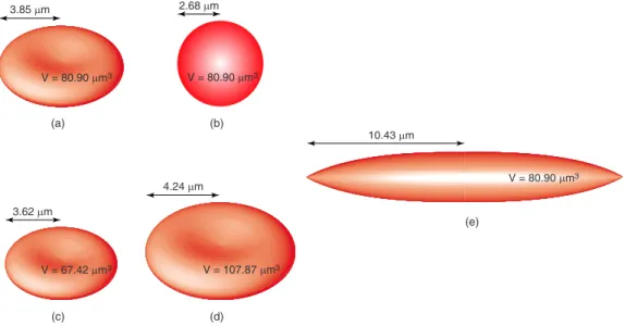
In this paper, we present a comparative study of scattering from healthy and deformed RBCs using surface integral equa-tions. As depicted in Fig.1, we consider a healthy共ordinary兲 RBC with a biconcave shape in addition to four types of de-formed cells, namely, a spherocyte, a microcyte, a macrocyte, and a sickle cell 共see Sec. 2 for detailed characteristics of these four deformed RBCs兲. For the five different RBC shapes, SCS values are calculated and compared. In this way, we determine strict guidelines to distinguish deformed RBCs from healthy RBCs and to diagnose various diseases using SCS values. Since SCS depends on the orientation of the RBC, we also test all possible illuminations to avoid misin-terpretations during the detection process.

Our simulation environment is based on the multilevel fast multipole algorithm21共MLFMA兲, which provides efficient so-lutions of electromagnetics problems discretized with large numbers of unknowns. Problems are formulated with the elec-tric and magnetic current combined-field integral equation22 共JMCFIE兲 discretized with the Rao-Wilton-Glisson23_共RWG兲

functions on planar triangles. JMCFIE provides well-conditioned matrix equations, which can be solved efficiently by using iterative algorithms.24 Nevertheless, accurate dis-cretizations of RBCs at realistic frequencies lead to matrix equations involving hundreds of thousands of unknowns. Hence, we employ MLFMA to accelerate the matrix-vector multiplications共MVMs兲 required by iterative solvers without deteriorating the accuracy of results.

The paper is organized as follows. Section 2 provides an overview of possible deformations of RBCs due to various diseases. Section 3 presents rigorous formulations of scatter-ing problems involvscatter-ing RBCs, and their discretizations for 1083-3668/2010/15共4兲/045004/8/$25.00 © 2010 SPIE

Address all correspondence to: Özgür Ergül, University of Strathclyde, Depart-ment of Mathematics and Statistics, Glasgow, Scotland, G1 1XH, United King-dom; Tel: 44 141 548 3650; E-mail: ozgur.ergul@strath.ac.uk

(2)

numerical solutions. Efficient solutions of problems using it-erative solvers, MLFMA, and preconditioners are presented in Sec. 4. Finally, Sec. 5 presents solutions and numerical re-sults, followed by our concluding remarks in Sec. 6.

2 Deformation of Red Blood Cells

Due to various diseases, RBCs can be deformed in terms of size and shape. For example, an RBC is identified25as a mac-rocyte if its diameter is larger than8.5␮m, even though it may have a biconcave shape like an ordinary RBC. Similarly, an RBC with a diameter smaller than7.0␮m is identified as a microcyte.25 Among various types of shape-deformed RBCs, sickle cells are identified by their extraordinary thin and long structures with pointed ends,26whereas spherocytes have almost spherical geometries.27

Microcytosis and macrocytosis have clinical significance because they may indicate other serious underlying diseases. Microcytosis is observed mainly in disorders in iron metabo-lism or deficiencies in hemoglobin synthesis,28whereas mac-rocytosis is mostly observed in drug use, alcoholism, liver diseases, myeloma, and leukemia.29On the other hand, sickle cells are encountered in sickle-cell anemia or sickle-cell trait, which are caused by abnormal hemoglobin structures. Due to their extraordinary shape, sickle cells may not be able to pass through capillaries, blocking the blood flow.30,31In the case of the sickle-cell anemia, 30 to 60% of RBCs may have sickle shapes, whereas this ratio drops to only 1% for the sickle-cell trait.26In general, the number of sickle cells depends on vari-ous factors, particularly deoxygenation levels.26,30 Finally, spherocytes are commonly observed in hereditary spherocyto-sis disease, which further leads to anemia, splenomegaly, jaundice, and many other clinical symptoms.32

Currently, most automated diagnosis setups rely on mean corpuscular volume 共MCV兲 to detect the deformation of RBCs in terms of size. Specifically, high and low MCV values may indicate the presence of macrocytes and microcytes, re-spectively. However, MCV measurements are usually

insuffi-cient for a reliable diagnosis, and peripheral blood smears are required, especially in the early stages of macrocytosis.29As opposed to microcytes and macrocytes, sickle cells can be diagnosed via biochemical and genetic tests, which are avail-able only in specialized laboratories,25,33and spherocytes are usually detected via mean corpuscular hemoglobin concentra-tion and RBC width measurements.32 Nevertheless, blood smear tests remain as the gold standard of diagnosing sickle cells and spherocytes, as for microcytes and macrocytes.

As presented in this paper, ordinary and deformed RBCs, i.e., microcytes, macrocytes, sickle cells, and spherocytes, can be distinguished from each other using a complete analysis of SCS values. Based on our results, we offer a fast and reliable technique to detect deformed RBCs in a blood sample using an automated diagnosis setup.

3 Formulation

Consider a homogeneous dielectric object with a three-dimensional arbitrary shape located in a homogeneous space. Electromagnetic permittivity and permeability of the object and the outer medium are共⑀i,␮i兲 and 共⑀o,␮o兲, respectively. Applying the equivalence principle,34equivalent electric and magnetic currents are defined on the surface of the object S, i.e.,

J共r兲 = nˆ ⫻ H共r兲, 共1兲

M共r兲 = − nˆ ⫻ E共r兲, 共2兲

where nˆ is the unit normal vector. Using the equivalent cur-rents, secondary 共scattered兲 electric and magnetic fields can be calculated as

E_o,is 共r兲 = ⫾␩o,iTo,i共J兲共r兲 ⫿ K_o,iPV共M兲共r兲

+共⍀i,o/4␲兲nˆ ⫻ M共r兲, 共3兲 3.85 µm V = 80.90 µm3 2.68 µm V = 80.90 µm3 (a) (b) 3.62 µm V = 67.42 µm3 4.24 µm V = 107.87 µm3 (c) (d) 10.43 µm V = 80.90 µm3 (e)

Fig. 1 Healthy and deformed RBCs:共a兲 a healthy 共ordinary兲 RBC with a biconcave shape; 共b兲 a spherocyte having exactly the same volume as the

ordinary RBC;共c兲 a microcyte, which is smaller than an ordinary RBC, with a biconcave shape; 共d兲 a macrocyte, which is larger than an ordinary RBC, with a biconcave shape; and共e兲 a sickle cell having exactly the same volume as an ordinary RBC.

(3)

H_o,is 共r兲 = ⫾ 1

␩o,i

To,i共M,r兲 ⫾ Ko,i PV_共J,r兲

−共⍀i,o/4␲兲nˆ ⫻ J共r兲, 共4兲

when the observation point r is outside共o兲 or inside 共i兲 the object. In Eqs.共3兲 and共4兲,␩u=共␮u/⑀u兲1/2 for u= i , o repre-sents the wave impedance,0艋⍀o艋4␲is the external solid angle, and⍀i= 4␲−⍀ois the internal solid angle. Integrodif-ferential operators are derived as

Tu共X,r兲 = iku

冕

S dr⬘X共r⬘兲gu共r,r⬘兲 + i ku

冕

S dr⬘ⵜ⬘X共r⬘兲 ⵜ g_u共r,r⬘兲, 共5兲 KuPV_{共X,r兲 =}

冕

PV,S dr⬘X共r⬘兲 ⫻ ⵜ⬘gu共r,r⬘兲, 共6兲 where PV indicates the principal value of the integral, ku =␻共␮u⑀u兲1/2 is the wave number, and gu共r,r

⬘

兲 denotes the homogeneous-space Green’s function defined as

gu共r,r⬘兲 =

exp共ikuR兲

4␲R 共R = 兩r − r⬘兩兲, 共7兲

in phasor notation with theexp共−i␻t兲 convention.

3.1 JMCFIE

Boundary conditions on the surface of the object can be writ-ten as

再

nˆ⫻ − nˆ⫻ nˆ⫻

冎

共E inc_{+ E} o s_{兲共r兲 =}

再

冎

Ei s_{共r兲, 共8兲} and

再

冎

共H inc_{+ H} o s_{兲共r兲 =}

再

冎

Hi s_{共r兲, 共9兲} where Einc共r兲 and Hinc共r兲 are incident electric and magnetic fields produced by external sources. Using Eqs.共3兲and 共4兲, and combining boundary conditions appropriately, JMCFIE is derived as

冋

Z11 Z12 Z21 Z22

册

·

冋

J M

册

共r兲 =

冋

f1 f2

册

共r兲, 共10兲 where Z11共X,r兲 = − X共r兲 + nˆ ⫻ 共Ko PV₋_KiPV_兲共X,r兲 − nˆ⫻ nˆ ⫻共To+Ti兲共X,r兲, 共11兲 Z12共X,r兲 = nˆ ⫻ nˆ ⫻ 共␩o −1_KoPV +␩_i−1KiPV兲共X,r兲 −共4␲兲−1共␩_o−1⍀o−␩i −1_⍀ i兲nˆ ⫻ X共r兲 + nˆ⫻共␩_o−1To−␩_i−1Ti兲共X,r兲, 共12兲 Z21共X,r兲 = − nˆ ⫻ nˆ ⫻ 共␩oKoPV +␩iKiPV兲共X,r兲 +共4␲兲−1_共␩ o⍀o−␩i⍀i兲nˆ ⫻ X共r兲 − nˆ⫻共␩oTo−␩iTi兲共X,r兲, 共13兲 Z22共X,r兲 = Z11共X,r兲, 共14兲 and f1共r兲 =␩o −1_nˆ_{⫻ nˆ ⫻ E}inc_{共r兲 − nˆ ⫻ H}inc_共r兲, _共15兲 f2共r兲 =␩onˆ⫻ nˆ ⫻ Hinc共r兲 + nˆ ⫻ Einc共r兲. 共16兲 Among infinitely many surface formulations of dielectric ob-jects, JMCFIE is a preferable formulation in terms of effi-ciency and accuracy.22,24 Specifically, solutions of JMCFIE usually require fewer iterations than solutions of other formu-lations, particularly when the number of unknowns is large.24 In addition, JMCFIE provides more accurate solutions than other efficient formulations, such as the Müller formulation.24

3.2 Discretization

For numerical solutions of JMCFIE, equivalent currents are expanded in a series of basis functions bn共r兲, i.e.,

关J共r兲,M共r兲兴 =

兺

冕

Sm drtm共r兲 · f2共r兲 =

冕

S_m drt_m共r兲 · 共nˆ ⫻ Einc₋_␩ oHinc兲共r兲, 共20兲 The matrix elements in Eq.共18兲are derived as

·

冋

x1 x2

册

. 共31兲

For efficient solutions of scattering problems involving RBCs, we employ MLFMA to perform MVMs in O共N log N兲 time usingO共N log N兲 memory.

4.1 MLFMA for Dielectric Objects

Considering Eq.共31兲, we perform four MVMs with the four partitions of the2N⫻2N matrix. MVMs are decomposed as

Z ¯ ab· xb= Z¯ab NF_{· x} b+ Z¯ab FF_{· x} b, 共32兲

for a= 1 , 2 and b = 1 , 2, where near-field interactions denoted by Z¯_abNF are calculated directly and stored in memory to per-form partial multiplications Z¯_abNF· xb. On the other hand, mul-tiplications involving far-field interactions, i.e., Z¯_abFF· xb, are performed efficiently using MLFMA. Those multiplications are further decomposed into two parts as

Z ¯ ab FF_{· x} b= Z¯ab,o FF _{· x} b+ Z¯ab,i FF _{· x} b, 共33兲

since MLFMA is applied separately for inner and outer media. To calculate far-field interactions, a multilevel tree struc-ture with L=O共log N兲 levels is constructed by placing the object in a cubic box and recursively dividing the computa-tional domain into subdomains共clusters兲. In this way, interac-tions of basis and testing funcinterac-tions that are far from each other can be calculated efficiently using the factorization and the diagonalization of the Green’s function. Each MVM in the form of Z¯_ab,uFF · xbcan be performed in three stages, called ag-gregation, translation, and disaggregation.

4.1.1 Aggregation

In this stage, radiated fields of clusters are calculated from the bottom of the tree structure to the highest level共l=L兲. At the lowest level, radiation patterns of basis functions are multi-plied with coefficients provided by the iterative solver and combined to obtain radiated fields of clusters, i.e.,

再

S_ab,uC,␪ S_ab,uC,␾

冎

=n

兺

苸C

xb关n兴

再

S_ab,un,␪

S_ab,un,␾

冎

, 共34兲 where S_ab,uC,␪ and S_ab,uC,␾ are arrays of K_u1elements containing␪ and␾components of the radiated field of a cluster C. Simi-larly, S_ab,un,␪ and S_ab,un,␾ in Eq. 共34兲are arrays of K_u1 elements containing␪and␾components of the radiation pattern of the nth basis function. We note that radiation patterns of basis functions 共hence radiated fields of clusters兲 depend on the matrix partition共a and b兲, as well as the medium 共u=o or u = i兲. The number of samples K_u1, which also depends on the medium, is determined by the excess bandwidth formula.36

Radiated fields of clusters in the higher levels of the tree structure are obtained by combining radiated fields of their subclusters. For a cluster C at level l⬎1,

再

S_ab,uC,␪ S_ab,uC,␾

冎

=

兺

C⬘苸C ␤¯ u C⬘→C_·_⌫¯ u 共l−1兲→l_·

再

Sab,u C⬘,␪ S_ab,uC⬘,␾

冎

, 共35兲 where␤¯_uC⬘→Cis a K_ul⫻K_ul diagonal matrix containing expo-nential shifts between cluster centers and ⌫¯_u共l−1兲→l is a K_ul ⫻Ku

共l−1兲 _{sparse interpolation matrix to increase the sampling} rate from level共l−1兲 to l.

4.1.2 Translation and disaggregation

During the translation and disaggregation stages, incoming fields at cluster centers are calculated from the top of the tree structure to the lowest level. At the highest level, the total incoming field for a cluster is obtained by combining the

(5)

in-coming fields due to translations. At lower levels, however, the incoming field to the center of a cluster involves a contri-bution from the incoming field to the center of its parent clus-ter. In general, the total incoming field for a cluster C at level l is obtained as

再

G_ab,uC,␪ G_ab,uC,␾

冎

=关⌫¯u l→共l+1兲_兴†_·_␤¯ uP共C兲→C·

再

G_ab,uP共C兲,␪ G_ab,uP共C兲,␾

冎

+

兺

C⬘苸F共C兲 W¯u·␣¯u C⬘→C_·

再

Sab,u C⬘,␪ S_ab,uC⬘,␾

冎

, 共36兲

where P共C兲 represents the parent cluster 共if it exists兲, and F共C兲 represents the clusters that are far from C. The first term on the right-hand side of Eq. 共36兲 accounts for a possible contribution from the parent cluster, where关⌫¯_u共l兲→共l+1兲兴† is a

Ku

l_⫻K u

共l+1兲_{sparse interpolation matrix. The second term} rep-resents translations from far-field clusters, where␣¯_uC⬘→Cis a diagonal translation matrix, and W¯u is a diagonal matrix in-volving integration weights.

5 Solutions and Results

In this section, we present the solution of scattering problems involving ordinary and deformed RBCs, and we discuss the diagnosis of various diseases using the SCS data. Accuracy of

the numerical results presented here and obtained with JM-CFIE, MLFMA, BiCGStab, and 4PBDP is demonstrated in our earlier work.24,37,38

5.1 Modeling of Red Blood Cells

We consider five different RBCs as illustrated in Fig. 1and listed in Table1. An ordinary RBC depicted in Fig. 1共a兲 is modeled by a rotationally symmetric biconcave surface de-fined as15

r共␪,␾兲 = a sinq_共_␪_{兲 + b,} _共39兲 where q= 5, a = 3.3␮m, and b = 0.55␮m. With these param-eters, the size and the volume of the ordinary RBC are 7.70␮m and 80.90␮m3_{, respectively. The spherocyte, which} is modeled as a dielectric sphere with a5.36-␮m diameter, as depicted in Fig.1共b兲, has exactly the same volume as an or-dinary RBC. The microcyte and the macrocyte in Figs.1共c兲 and1共d兲also have biconcave shapes, as defined in Eq.共39兲, but their volumes correspond to5/6 and 4/3 of the volume of an ordinary RBC. Finally, the sickle cell depicted in Fig.1共e兲 also has a rotationally symmetric shape as the others do, but it is elongated in one dimension. The size of the sickle cell is 20.9␮m, whereas its volume is the same as the volume of an ordinary RBC, i.e.,80.90␮m3_.

5.2 Solutions

RBCs in Fig.1are illuminated by a plane wave propagating in the −z direction with the electric field polarized in the x direction having a unit amplitude. Since the orientation of an RBC can be arbitrary in the flow cytometry, we investigate 13 different cases for each RBC, except for the spherocyte because it has a fully symmetric geometry. As an example, the default orientation 共␪o= 0 deg, ␾o = 0 deg兲 of an ordinary RBC is depicted in Fig. 2. We perform rotations around the x axis 共by an amount of ␪o兲 and the z axis共by an amount of␾o兲, respectively. Specifically, we consider ␪o=兵30 deg,60 deg,90 deg其 and ␾o =兵0 deg,30 deg,60 deg,90 deg其, in addition to the default case in Fig.2.

Relative permittivities of RBCs and the host medium are selected as 1.40 and 1.33, respectively. Numerical simulations are performed at 474 THz, corresponding to the output fre-quency of a typical helium-neon laser. The size of each RBC

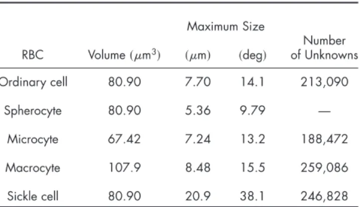
Table1 Ordinary and deformed RBCs.

RBC Volume共␮m3_兲 Maximum Size Number of Unknowns 共␮m兲共deg兲 Ordinary cell 80.90 7.70 14.1 213,090 Spherocyte 80.90 5.36 9.79 — Microcyte 67.42 7.24 13.2 188,472 Macrocyte 107.9 8.48 15.5 259,086 Sickle cell 80.90 20.9 38.1 246,828

(6)

in terms of the wavelength inside the host medium共␭o兲 are listed in Table1. Due to their relatively large sizes, accurate discretizations of RBCs using␭o/10 triangles lead to matrix equations involving 180,000 to 260,000 unknowns, as also listed in Table1. Except for the spherocyte, scattering prob-lems are formulated with JMCFIE and solved iteratively using the BiCGStab algorithm accelerated via MLFMA and 4PBDP, as detailed in Secs. 3 and 4. Scattering from the spherocyte is solved exactly by using a Mie-series algorithm. Solutions with MLFMA require only 15 to 20 iterations, and each solu-tion is performed in 3.0 to 4.5 h on a 3.6-GHz Intel Xeon processor using1.5 Gbyte of memory.

5.3 Results

Figure3 presents the solution of scattering problems involv-ing the RBCs depicted in Fig. 1. SCS values in forward-scattering共␪= 180 deg兲 and back-scattering 共␪= 0 deg兲 direc-tions are plotted in Figs.3共a兲and3共b兲, respectively. SCS in a bistatic direction共␪,␾兲 is defined as

SCS共␪,␾兲 = lim r→⬁

冋

4␲r

2兩Eo

s_共r,_␪_,_␾_兲兩2

兩Einc_共r,_␪_,_␾_兲兩2

册

. 共40兲 Since SCS depends on the orientation of the target, multiple values are obtained for each cell, except for the spherocyte. We observe that, depending on the cell type, SCS values change significantly. Considering the results for the ordinary RBC, we determine “safe” regions indicated by horizontal lines in Figs.3共a兲and3共b兲. For example, an SCS value higher than 44 dB␮m2 or lower than 43 dB␮m2 in the forward-scattering direction indicates a detection of an abnormal RBC, possibly

*

a macrocyte共if greater than 44 dB␮m2_{兲 or a} mi-crocyte 共if smaller than 43 dB␮m2_{兲. The decibel scale for} SCS is defined as关SCS共␪,␾兲兴dB= 10 log SCS共␪,␾兲. We note that, although less likely, a sickle cell may also present a low SCS value in the forward-scattering direction. As depicted in Fig.3共b兲, an SCS value smaller than−24 dB␮m2_{in the} back-scattering direction indicates a detection of a macrocyte, a microcyte, or a sickle cell.

SCS values in forward-scattering and back-scattering di-rections do not provide complete information for diagnosing diseases. For example, using the data in Figs.3共a兲and3共b兲, a spherocyte cannot be distinguished from an ordinary共healthy兲 cell. The required data can be obtained by considering SCS values in a set of side-scattering directions. We sample SCS *Since SCS has the dimension of area, its unit is square meters. We prefer square micrometers since a single cell has low SCS values. Furthermore, we use decibels square micrometers to improve the visibility of the results on a loga-rithmic scale. z x θ y φ (θ ,φ )=(0,0) ο ο ο ο

Fig. 2 Default orientation共␪o= 0 deg,␾o= 0 deg兲 of an ordinary RBC.

MAC MIC ORD SPH SIC

39 40 41 42 43 44 45 46 47 Forward Scattering Cell Shape Scattering Cross Section (dB µ m 2 ) (a)

MAC MIC ORD SPH SIC

−70 −60 −50 −40 −30 −20 −10 0 10 Back Scattering Cell Shape Scattering Cross Section (dB µ m 2 ) (b)

MAC MIC ORD SPH SIC

−50 −45 −40 −35 −30 −25 −20 −15 −10

Average Side Scattering

Cell Shape Scattering Cross Section (dB µ m 2 ) (c)

Fig. 3 Solutions of scattering problems involving an ordinary RBC

共ORD兲 and four different types of deformed RBCs, i.e., a spherocyte 共SPH兲, a macrocyte 共MAC兲, a microcyte 共MIC兲, and a sickle cell 共SIC兲: 共a兲 SCS in the forward-scattering direction, 共b兲 SCS in the back-scattering direction, and共c兲 average SCS in the side-scattering direc-tion are plotted in decibels square micrometer for different orienta-tions of RBCs.

(7)

on the x-y plane as a function of bistatic scattering angle␾ from 0 to 360 deg with 1-deg intervals. Then, the average SCS value in the side-scattering direction is computed as

SCSavg,side=

再

1 360

兺

_n=1 360 关兩SCS共␪= 90 deg,␾n兲兩2兴

冎

1/2 , 共41兲 where␾n=共n−1兲 deg for n=1,2, ... ,360. In the preceding,

␪= 90 deg refers to the azimuth plane, i.e., the x-y plane, on which all SCS values in the bistatic␾n directions are aver-aged. As depicted in Fig. 3共c兲, an average SCS value higher than −15 dB␮m2 _{or lower than} _{−24 dB}_␮_m2 _{in the} side-scattering direction indicates a detection of an abnormal RBC, such as a macrocyte, a spherocyte, or a sickle cell.

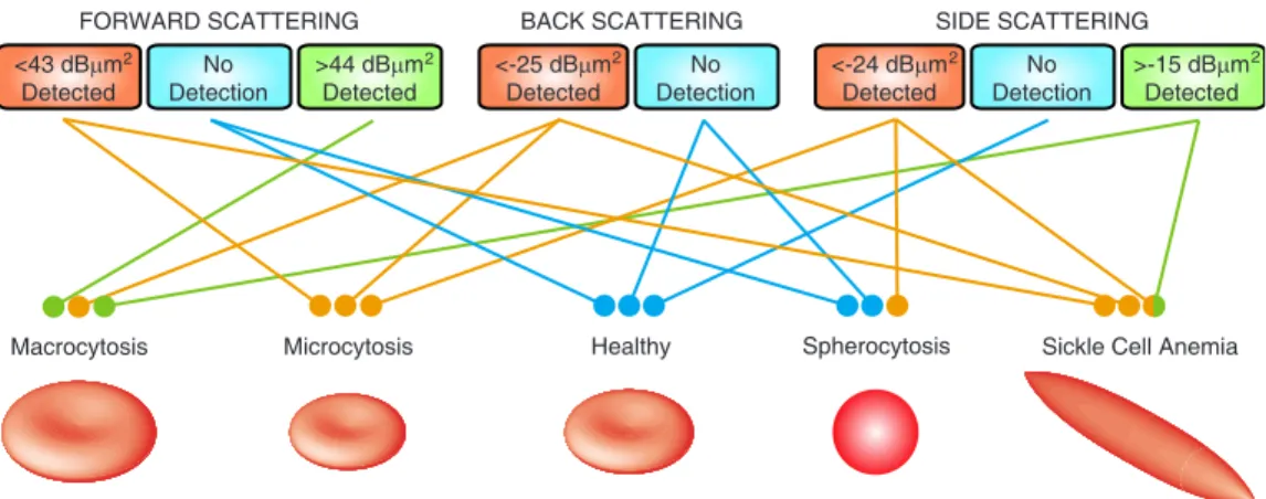
Finally, using all SCS results in Fig.3, we determine strict guidelines to detect deformed RBCs in a diagnosis setup. Fig-ure4presents a decision chart based on SCS values obtained in forward-scattering, back-scattering, and side-scattering di-rections. We assume that a sufficient number of RBCs are passed through the setup. The diagnosis of each disease can be described as follows:

1. Macrocytosis: Detection of SCS values higher than 44 dB␮m2 _{in the forward-scattering direction is a major} in-dicator for macrocytosis. SCS values lower than−25 dB␮m2 in the back-scattering direction and average SCS values higher than −15 dB␮m2 _{in the side-scattering direction} in-crease the reliability of the diagnosis.

2. Microcytosis: Detection of low SCS values in all direc-tions indicates microcytosis. Specifically, detection of SCS values lower than43 dB␮m2_{in the forward-scattering} direc-tion, SCS values lower than −25 dB␮m2 _{in the} back-scattering direction, and average SCS values lower than −24 dB␮m2_{in the side-scattering direction indicate} microcy-tosis.

3. Spherocytosis: Spherocytosis can be diagnosed by the detection of average SCS values lower than −24 dB␮m2 _in the side-scattering direction, without any abnormal SCS val-ues in the forward-scattering and back-scattering directions.

4. Sickle-Cell Anemia: Similar to microcytosis, sickle-cell anemia can be diagnosed by the detection of low SCS values in all directions. On the other hand, sickle-cell anemia also leads to average SCS values higher than−15 dB␮m2 _{in the}

side-scattering direction; this can be used to distinguish sickle-cell anemia from microcytosis.

6 Conclusion

We presented a comparative study of scattering from healthy and diseased RBCs with deformed shapes. By using a sophis-ticated simulation environment based on JMCFIE and MLFMA, scattering problems involving different RBCs with different orientations are solved both accurately and effi-ciently. By investigating SCS values in forward-scattering, back-scattering, and side-scattering directions, not necessarily limited to conventional cytometer setups, we were able to determine strict guidelines to distinguish deformed RBCs from healthy RBCs and to diagnose related diseases. Acknowledgments

This work was supported by the Scientific and Technical Re-search Council of Turkey共TUBITAK兲 under Research Grants 105E172 and 107E136, by the Turkish Academy of Sciences in the framework of the Young Scientist Award Program共LG/ TUBA-GEBIP/2002-1-12兲, and by contracts from ASELSAN and SSM. Özgür Ergür was also supported by a Research Starter Grant provided by the Faculty of Science at the Uni-versity of Strathclyde.

References

1. L. O. Reynolds, C. Johnson, and A. Ishimaru, “Diffuse reflectance from a finite blood medium: applications to the modeling of fiber optic catheters,”Appl. Opt.15, 2059–2067共1976兲.

2. G. D. Pederson, N. J. McCormick, and L. O. Reynolds, “Transport calculations for light scattering in blood,”Biophys. J.16, 199–207

共1976兲.

3. R. A. Meyer, “Light scattering from red blood cell ghosts: sensitivity of angular dependent structure to membrane thickness and refractive index,”Appl. Opt.16, 2036–2037共1977兲.

4. D. H. Tycko, M. H. Metz, E. A. Epstein, and A. Grinbaum, “Flow-cytometric light scattering measurement of red blood cell volume and hemoglobin concentration,”Appl. Opt.24, 1355–1365共1985兲.

5. J. M. Steinke and A. P. Shepherd, “Comparison of Mie theory and the light scattering of red blood cells,”Appl. Opt.27, 4027–4033共1988兲.

6. G. J. Steekstra, A. G. Hoeksta, E. Nijhof, and R. M. Heethaar, “Light scattering by red blood cells in ektacytometry: Fraunhofer versus anomalous diffraction,” Appl. Opt. 32, 2266–2272共1993兲. 7. G. J. Streekstra, A. G. Hoekstra, and R. M. Heethaar, “Anomalous

diffraction by arbitrarily oriented ellipsoids: applications in ektacy-tometry,”Appl. Opt.33, 7288–7296共1994兲.

8. P. Mazeron and S. Muller, “Dielectric or absorbing particles: EM FORWARD SCATTERING <43 dBµm Detected Macrocytosis No Detection >44 dBµm Detected BACK SCATTERING <-25 dBµm Detected No Detection SIDE SCATTERING <-24 dBµm Detected No Detection

Microcytosis Healthy Spherocytosis Sickle Cell Anemia >-15 dBµm

Detected

2 2 2 2 2

(8)

surface fields and scattering,”J. Opt.29, 68–77共1998兲.

9. A. G. Borovoi, E. I. Naats, and U. G. Oppel, “Scattering of light by a red blood cell,”J. Biomed. Opt.3, 364–372共1998兲.

10. M. Hammer, D. Schweitzer, B. Michel, E. Thamm, and A. Kolb, “Single scattering by red blood cells,” Appl. Opt. 37, 7410–7418

共1998兲.

11. A. N. Shvalov, J. T. Soini, A. V. Chernyshev, P. A. Tarasov, E. Soini, and V. P. Maltsev, “Light-scattering properties of individual erythro-cytes,”Appl. Opt.38, 230–235共1999兲.

12. A. M. K. Nilsson, P. Alsholm, A. Karlsson, and S. Andersson-Engels, “T-matrix computations of light scattering by red blood cells,”Appl. Opt.37, 2735–2748共1998兲.

13. J. He, A. Karlsson, J. Swartling, and S. Andersson-Engels, “Light scattering by multiple red blood cells,”J. Opt. Soc. Am. A21, 1953–

1961共2004兲.

14. A. Karlsson, J. He, J. Swartling, and S. Andersson-Engels, “Numeri-cal simulations of light scattering by red blood cells,”IEEE Trans. Biomed. Eng.52, 13–18共2005兲.

15. J. Q. Lu, P. Yang, and X. H. Hu, “Simulations of light scattering from a biconcave red blood cell using the finite-difference time-domain method,”J. Biomed. Opt.10, 024022共2005兲.

16. N. K. Uzunoglu, D. Yova, and G. S. Stamatakos, “Light scattering by pathological and deformed erythrocytes: an integral equation model,” J. Biomed. Opt.2, 310–318共1997兲.

17. G. S. Stamatakos, D. Yova, and N. K. Uzunoglu, “Integral equation model of light scattering by an oriented monodisperse system of tri-axial dielectric ellipsoids: application in ektacytometry,”Appl. Opt.

36, 6503–6512共1997兲.

18. S. V. Tsinopoulos and D. Polyzos, “Scattering of HeNe laser light by an average-sized red blood cell,”Appl. Opt.38, 5499–5510共1999兲.

19. S. V. Tsinopoulos, E. J. Sellountos, and D. Polyzos, “Light scattering by aggregated red blood cells,”Appl. Opt.41, 1408–1417共2002兲.

20. T. W. Lloyd, J. M. Song, and M. Yang, “Numerical study of surface integral formulations for low-contrast objects,”IEEE Antennas Wire-less Propag. Lett.4, 482–485共2005兲.

21. J. Song, C.-C. Lu, and W. C. Chew, “Multilevel fast multipole algo-rithm for electromagnetic scattering by large complex objects,”IEEE Trans. Antennas Propag.45, 1488–1493共1997兲.

22. P. Ylä-Oijala and M. Taskinen, “Application of combined field inte-gral equation for electromagnetic scattering by dielectric and com-posite objects,” IEEE Trans. Antennas Propag. 53, 1168–1173

共2005兲.

23. S. M. Rao, D. R. Wilton, and A. W. Glisson, “Electromagnetic scat-tering by surfaces of arbitrary shape,”IEEE Trans. Antennas Propag.

30, 409–418共1982兲.

24. Ö. Ergül and L. Gürel, “Comparison of integral-equation formula-tions for the fast and accurate solution of scattering problems involv-ing dielectric objects with the multilevel fast multipole algorithm,” IEEE Trans. Antennas Propag.57, 176–187共2009兲.

25. A. Tefferi, “Anemia in adults: a contemporary approach to diagno-sis,”Mayo Clin. Proc.78, 1274–1280共2003兲.

26. L. Pauling, H. A. Itano, S. J. Singer, and I. C. Wells, “Sickle cell anemia, a molecular disease,”Science110, 543–548共1949兲.

27. K. H. Walker, W. D. Hall, and J. W. Hurst, Clinical Methods: The History, Physical, and Laboratory Examinations, Butterworth-Heinemann, Boston共1990兲.

28. L. Chrobak, “Microcytic and hypochromic anemias,” Vnitr. Lek. 47, 166–174共2001兲.

29. F. Aslinia, J. J. Mazza, and S. H. Yale, “Megaloblastic anemia and other causes of macrocytosis,”Clin. Med. Res.4, 236–241共2006兲.

30. G. J. Lonergan, D. B. Cline, and S. L. Abbondanzo, “Sickle cell anemia,” Radiographics 21, 971–994共2001兲.

31. A. Ashley-Koch, Q. Yang, and R. S. Olney, “Sickle hemoglobin 共HbS兲 allele and sickle cell disease: a HuGE review,” Am. J. Epide-miol. 151, 839–845共2000兲.

32. S. Perrotta, P. G. Gallagher, and N. Mohandas, “Hereditary sphero-cytosis,”Lancet372, 1411–1426共2008兲.

33. American Association for Clinical Chemistry, http:// www.labtestsonline.org.

34. J. A. Stratton, Electromagnetic Theory, McGraw-Hill, New York 共1941兲.

35. H. van der Vorst, “Bi-CGSTAB: a fast and smoothly converging vari-ant of Bi-CG for the solution of nonsymmetric linear systems,”SIAM J. Sci. Comput. (USA)13, 631–644共1992兲.

36. W. C. Chew, J.-M. Jin, E. Michielssen, and J. Song, Fast and Effi-cient Algorithms in Computational Electromagnetics, Artech House, Boston共2001兲.

37. Ö. Ergül and L. Gürel, “Novel electromagnetic surface integral equa-tions for highly accurate computaequa-tions of dielectric bodies with arbi-trarily low contrasts,” J. Comput. Phys. 23, 9898–9912共2008兲. 38. Ö. Ergül and L. Gürel, “Efficient solution of the electric-field integral

equation by the iterative LSQR algorithm,”IEEE Antennas Wireless Propag. Lett.7, 36–39共2008兲.