Full Terms & Conditions of access and use can be found at
http://www.tandfonline.com/action/journalInformation?journalCode=tppc20
Download by: [Bilkent University] Date: 27 October 2017, At: 05:56
Production Planning & Control
ISSN: 0953-7287 (Print) 1366-5871 (Online) Journal homepage: http://www.tandfonline.com/loi/tppc20
Concurrent consideration of product design,
process planning and production planning
activities
Gajendra Kumar Adil
To cite this article: Gajendra Kumar Adil (1998) Concurrent consideration of product design, process planning and production planning activities, Production Planning & Control, 9:2, 167-175, DOI: 10.1080/095372898234389
To link to this article: http://dx.doi.org/10.1080/095372898234389
Published online: 15 Nov 2010.
Submit your article to this journal
Article views: 42
Concurrent consideration of product design,
process planning and production planning
activities
GAJENDRA KUMAR ADIL
Keywords concurrent engineering, integration of
manufac-turing functions, production planning, product design, process planning
A bstract. In manufacturing engineering, product design,
pro-cess planning and production planning activities are often con-sidered independently. However, in order to eectively respond to changes in business situations, such as changes in demand forecast, product mix and technology, it is desirable to consider them concurrently. For this purpose, a large-scale linear pro-gramming model has been developed. The model considers minimization of the sum of processing cost, late shipment cost and inventory holding cost as the objective, and concurrently selects product designs, and generates process plans and produc-tion plans. The number of columns in the formulaproduc-tion can be large and, hence, an e cient column generation scheme is developed to solve the model. The model and solution proce-dure are illustrated with examples.
1. Introduction
Concurrency and integration of various manufacturing functions are important for any manufacturing
organiza-tion to eectively respond to the current dynamic
busi-ness situations ( Arcelus and Srinivasan 1995) . This has led to the emergence of concurrent engineering ( CE) and computer integrated manufacturing ( CI M) concepts,
and rapid progress in CE and CIM tools and technolo-gies. This paper considers three important manufacturing functions simultaneously: product design, process plan-ning, and production planning.
Today, product diversi® cation rather than product standardization is the market need. Custom-made prod-ucts, with a great many variations in design are common. To have many product variations helps to satisfy custo-mers. In addition, this can provide a manufacturing organization with ¯ exibility in resource management. With judicious selection of design ( product) mix, it is
possible to ensure e cient use of resources ( such as
good load balance and high utilization) because the availability of a large number of designs gives ¯ exibility in resource selection.
Process planning is a function which associates each design feature ( or group of design features) to manufac-turing resource( s) to be used for its creation. There is no unique way in which a product with a given design can be manufactured. This leads to the existence of many process plans corresponding to a given product design. Many researchers ( Horvath et al. 1996) have worked on the automatic generation of process plans for the product design for a class of products.
A uthor: Gajendra Kumar Adil, Department of Industrial Engineering, Bilkent University, 06533 Bilkent, Ankara, Turkey; Address for correspondence: 133-99 Dalhousie Drive, Winnipeg, Manitoba, Canada, R3T 3M2.
Ga j e ndr aKu ma rAd il worked as an assistant professor at Bilkent University from September
1995 to August 1996 and this research was carried out during that period. Currently, he is working as a consultant for Bristol Aerospace Limited, Winnipeg, Canada. He holds a PhD ( 1994) in Industrial Enginering from the University of Manitoba, an MSc ( 1990) in Industrial Engineering from the University of Regina, an M.Tech ( 1987) in Mechanical Engineering from the Indian Institute of Technology, Kanpur and a B.Engg ( 1985) in Mechanical Engineering from Ravishankar University, Raipur, India. His research interests are in cellular manufacturing, production planning and concurrent engineering.
0953-7287/98 $12.00 Ñ 1998 Taylor & Francis Ltd.
Production planning decisions may be many. One important medium- and long-range production planning decision is to determine the number of parts to be pro-duced during each planning period. This decision depends to a great extent on ( i) demand forecast, and ( ii) resource availability. How a product is designed can
aect demand. The design and process plan selections
determine the resource requirements. Thus, product design, process planning and production planning in¯ u-ence each other, and concurrent consideration of these three should help a company in optimizing its operation. ( We will explain some of the iterations with examples in Section 4.)
Some authors have considered the relationship between design and process planning ( Dewhurst and Boothroyd 1988, Horvath et al. 1996) , and a few ( ElMaraghy and ElMaraghy 1992, Larsen and Clausen 1992, Huang et al. 1995) have simultaneously considered process planning and production planning activities. The objective of this paper is to develop a procedure to achieve simultaneous design selection, process plan gen-eration and production planning. We develop a model for concurrent selection of product design; generation of
an optimal process plan by implicitly enumerating di
er-ent options; and developmer-ent of production plans. In Section 2, a mathematical formulation of the prob-lem is presented. The model can result in a large number of explicit columns, therefore, in Section 3, we develop a solution procedure based on a column generation scheme
to solve large-size problems e ciently. The model and
the importance of concurrent design selection, process plan generation and production planning decisions are illustrated in Section 4. Computational experience with the column generation scheme is presented in Section 5 and in Section 6 we discuss a possible variation of the model. Finally, conclusions are presented in Section 7.
2. Mathematical formulation
We shall introduce notation and terms before present-ing the mathematical model
2.1. N otation Indices
p product type(p = 1
,
2,
. . .,
P)d design ( or variation) of product (d = 1
,
2,
. . .
,
Dp)f design feature(f =1
,
2,
. . .,
Fpd)k process plan(k =1
,
2,
. . .Kpd)r resource type(r = 1
,
2,
. . .,
R)t
,
tÂ
time period in planning horizon (t,
tÂ
= 1,
2,
. . .
,
T). ParametersBrt total processing time available on resource type
r in time period t
Crf(pd) cost incurred in using resource r to create
feature f speci® ed in design d of product type p
Dpt forecast production quantity ( or demand) of
product type p in planning period t
htt
Â
(p) inventory holding cost for each unit of product type p when the product is produced in period t to meet the demand in period tÂ
(tÂ
>
t) httÂ
(p) late shipment cost for each unit of product typep when the product is produced and supplied
in period t against the demand in period
t
Â
(tÂ
<
t)Rpd number of resources in the cost ( time) matrix
corresponding to design d of product p
Trf(pd) time required on resource r in creating feature
f speci® ed in design d of product type p.
Decision variables
Arf(kpdtt
Â
)=1 if, product type p is produced in design
din time period t to meet the customer’s demand in period t
Â
,
using process plan k that requires resource r to create feature f 0 otherwiseì
ïïïïï
ïï
í
ïïïïï
ïï
î
X(kpdtt
Â
)= quantity of product type p produced in design d using process plan k in period t to meet the customer’s demand in period tÂ
2.2. T erms
We now explain three terms: product design, process planning and production planning, and relevant nota-tion used in this paper.
2.2.1. P roduct design
The design department comes up with many variations of a given product p and provides a design speci® cation for each variation. Let there be Dpdesigns ( or variations) of product p. Each design speci® es a number of features,
f (f = 1
,
2,
. . .,
Fpd) required to manufacture the prod-uct. Each design feature can be created using one of the alternative resources. However, the time and cost incurred may vary depending upon the resource selected. Let the time required and cost incurred on the selected168 G . K . A dil
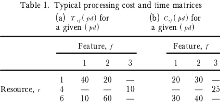
resource r to process feature f speci® ed in design ( or variation) d of product p be Trf(pd) and Crf(pd), respec-tively. They can be represented by matrices as shown in Table 1.
The following information can be extracted from the time and cost matrices in Table 1. Design ( variation) d of product p speci® es three design features. Each feature can be produced by one of the three resource types 1, 4 and 6 with processing time and cost indicated. In the matrices, the sign `Ð ’ ( for example, corresponding to f = 3 and
r = 1) indicates that the resource is not capable of
pro-ducing the corresponding feature. Sign `Ð ’ can also be replaced by in® nity ( or a large number) .
2.2.2. P rocess plans
Production according to the speci® cations outlined in a design ( product variation) requires generation of a pro-cess plan. This can be obtained by choosing a feasible resource for each design feature. We can represent a pro-cess plan by a set containing all the design features and a feasible resource selected to produce each feature. For a given design there can be many feasible process plans. For example if the data given in Table 1 are con-sidered, four feasible process plans are possible as shown in Table 2.
Note that infeasible process plans ( represented with time and cost as in® nity) are not listed in the table. If these are included there will be a total of 27 process plans. This can be calculated as the number of resources in the
matrix to the power number of features = RFpd
pd = 33.
2.2.3. P roduction plans
The production planning decision involves determina-tion of the quantity of each product type to be produced in each planning period given the amount of time avail-able on resources and the demand forecast for the prod-ucts. We may not always be able to produce just the demanded quantity in each time period because of con-straints on resource availability or economic considera-tions. We may have situations when in some period we may produce more ( or less) than the quantity demanded. If the demand is not met, companies lose current ( or even future) business opportunities. Sometimes the company may not be able to ship the products late, after paying an agreed penalty to the customer. We de® ne htt
Â
(p) to be the late shipment cost for each unit of product type p when the product is produced and supplied in period t against the demand in period tÂ
(t>
tÂ
). If late shipment is not possible, a very high cost value can be allocated in the model to disallow it. Sometimes, excess production capacity may be available in a given period. In that case a product can be produced in excess quantity to meet future demands. This results in inventory holding cost. We de® ne, httÂ
(p) to be the inventory holding cost for each unit of product type p when the product is produced in period t to meet the demand in period tÂ
(t<
tÂ
). We have been able to use the same variable httÂ
(p) to repre-sent both the inventory cost and late shipment cost because for any given situation both cannot occur simul-taneously.We can generate dierent production and process
plans to produce a given product p in design d. Let us de® ne binary variables Arf(kpdtt
Â
) to represent all such options. Arf(kpdttÂ
) takes the value 1 if all of the following conditions hold true: product type p in design d ispro-duced in period t to meet the demand in period t
Â
anduses process plan k in which resource r is selected to create the feature f . If any of the conditions is not true, the variable takes the value 0.
2.3. M athematical model
Having de® ned the notation and explained the terms, we can now formulate a large-scale linear programming model as follows.
Table 1. Typical processing cost and time matrices ( a) Trf(pd) for ( b) Crf(pd)for a given (pd) a given(pd) Feature, f Feature, f 1 2 3 1 2 3 1 40 20 Ð 20 30 Ð Resource, r 4 Ð Ð 10 Ð Ð 25 6 10 60 Ð 30 40 Ð
Note: `Ð ’ indicates that the resource is not capable of producing that feature.
Table 2. Enumeration of process plans for data presented in Table 1.
Process plan,
k Representation of process plan [selected( feature, resource) combinations] Total time ( cost) 1
[
(1,
1),
(2,
1),
(3,
4)]
70 ( 75) 2[
(1,
1),
(2,
6),
(3,
4)]
110 ( 85) 3[
(1,
6),
(2,
1),
(3,
4)]
40 ( 85) 4[
(1,
6),
(2,
6),
(3,
4)]
80 ( 95) Note. The infeasible process plans represented with time and cost as in® nity are not listed in the table. If we include these also then there will be a total of 27 process plans.Minimize z =
å
tå
tÂ
å
på
då
kå
få
r Arf(kpdttÂ
) Crf(pd)X(k pdttÂ
) +å
tå
tÂ
<tå
på
då
k httÂ
(p)X(kpdttÂ
) +å
tå
tÂ
>tå
på
då
k httÂ
(p)X(kpdttÂ
) or P0: Minimize z =å
tå
tÂ
å
på
då
kå
få
r Arf(kpdttÂ
) Crf(pd)X(kpdttÂ
) +å
tå
tÂ
å
på
då
k httÂ
(p)X(kpdttÂ
) (1) Subject to:å
tå
då
k X(kpdttÂ
)³
DptÂ
"
(p,
tÂ
) (2)å
tÂ
å
på
då
kå
f Arf(kpdttÂ
)Trf(pd)X(k pdttÂ
)£
Brt"
(r,
t) (3) X(kpdttÂ
)³
0"
(k,
p,
d,
t,
tÂ
) (4)In the above formulation, objective function ( 1) is the sum of processing cost, late shipment cost and inventory holding cost. Constraints ( 2) ensure that the demand for all products are met and constraints ( 3) enforce the capa-city limitation on resources. Constraints ( 4) impose non-negativity restrictions on production quantities.
3. Solution procedure
Model P0 is a large-scale linear programming model. The number of process plans and the resulting number of columns ( if we explicitly consider these columns) in the model can be large. For instance, consider a design in which the number of design features is 10 and the num-ber of resources to produce one or more features is ® ve. The number of possible process plans for this design will
be 510= 9 765 625. Further, let there be 20 products,
each of which is to be produced in ® ve designs during ® ve planning periods. The resulting number of explicit columns
[
X(kpdttÂ
)]
, would be equal to 9 765 625´
20´
5´
5´
5 which is of the order 2.4´
1010. In the simplex procedure, pricing all the variables in order to determine the entering column is quite expensive. Therefore, we propose a column generation scheme to implicitlyenu-merate them. For the above situation, the proposed
scheme will require pricing of only 1
´
20´
5´
5´
5 =2.5
´
103 variables because it does not requireenumera-tion over process plan index k. The most promising pro-cess plan is obtained using the column generation scheme described below. A similar scheme is reported by Rajamani et al. ( 1996) in the context of cell design.
The structure of the model P0 is such that the genera-tion of an X -column in each simplex iteragenera-tion requires solving a semi-assignment problem. This can be solved using a simple approach. To explain this, let us de® ne simplex multipliers corresponding to constraints ( 2) as
Upt
Â
( for p = 1,
2,
. . .,
P; tÂ
= 1,
2,
. . .,
T) and that corre-sponding to constraints ( 3) as Vrt ( for r = 1,
2,
. . .R; andt = 1
,
2,
. . .,
T). A non-basic variable, X(k pdttÂ
) having reduced cost less than zero can improve the objective value. We need to check if the following condition is met for the corresponding column to enter,å
få
r Arf(kpdttÂ
)Crf(pd)+ httÂ
(p)-
UptÂ
-
å
få
r Arf(kpdttÂ
)Trf(pd)´
Vrf<
0 orå
få
r Arf(kpdttÂ
)[
Crf(pd)-
Trf(pd)´
Vrt]
+httÂ
(p)-
UptÂ
<
0 (5) Since the range of values a process plan index k takes can be quite high we do not explicitly enumerate and price each of them. Instead, we generate the most promising process plan k*, that gives the lowest value for the sum-mation term in expression ( 5) . This gives the following subproblem. SP: Minimize U(p,
d) =å
få
r[
Crf(pd)-
Trf(pd)´
Vrt]
´
Arf(k*pdttÂ
) Subject to:å
r Arf(k*pdttÂ
) = 1"
f Arf(k*pdttÂ
)Î {
0,
1}
"
(r,
f)Note that the values of variables Arf(k*pdtt
Â
) or the resource± feature combinations obtained by solving SPde® ne the most promising process plan k*. Further, the
objective function coe cient in SP depends only on part
pand design d. Thus this problem needs to be solved for
each (p
,
d) combination.170 G . K . A dil
Problem SP is separable by f . The resulting problem for each f can be solved by inspection, i.e. select the variable with the least value of its coe cients underlined in the objective function. Let the optimal objective value of SP by U*(p
,
d) for a given(p,
d). We select a design d* that gives the minimum value of U*(p,
d). We store the process plan for this design, i.e. store the Arf(k*,
p,
d*,
t,
tÂ
) matrix.Now we need to determine the best values of periods t*,
t*
Â
for given part p. Using the above developments,expression ( 5) reduces to or F(p)
<
0 where F(p) = minimum d[
U *(pd)]
+ minimum tÂ
minimum t{
httÂ
(pp)-
UptÂ
}
[
]
Column X(k*
,
p,
d*,
t*,
t*Â
) oers the maximum cost improvement potential for part p. All such variablesX(k*
,
p,
d*,
t*,
t*Â
) which have a negative value for F(p)can enter. From this we select the column which gives the most negative value, i.e. we enumerate over all parts p and pick the column X(k*
,
p*,
d*,
t*,
t*Â
) with the most negative value for F(p). In other words,F(p*) = minimum
p
{
F(p)}
The column generation scheme thus described is illus-trated with a numerical example in the Appendix.
A two-phase simplex method is used here to solve the linear programming problem. In phase I, initially, arti-® cial variables of constraints ( 2) appear in the basis with a very high cost coe cient, M ; and in constraints ( 3) all
slack variables appear with cost coe cient zero. The
simplex algorithm stops when the best X -column found has a value of F(p*)
³
0 ( i.e. no X -column can enter) ;Upt
Â
>
0 [i.e. no excess variable corresponding to con-straints ( 2) can enter]; and Vrt<
0 [i.e. no slack variable corresponding to constraints ( 3) can enter]. The simplex algorithm combined with the column generation scheme proceeds as follows:S tep 0. Initialize basis and solution. Initialize iteration count as 0.
S tep 1. Increase the simplex iteration count.
S tep 2. Find the entering variable ( column) :
( a) Check if an X column can enter using the column generation scheme described earlier in this section. If this happens then go to step 3.
( b) Check if an excess variable in constraints ( 2) can enter. If this happens then go to step 3. ( c) Check if a slack variable in constraint ( 3) can
enter. If this happens then go to step 3. If algorithm is still in phase I, then the problem is unfeasible, or the optimality condition has been reached. Go to step 4.
S tep 3. Find the departing variable, update the basis, ® nd the new solution for the current basis, and go to step 1.
S tep 4. Print the results and terminate the algorithm.
Table 3. Data for example ( case 1) Number of product types, P = 2 Number of designs, D1= D2= 1
Number of planning periods, T = 2 Demands ( Dpt) for products
Time period, t
Product type, p 1 2
1 10 20
2 20 10
Processing costs and times
Product 1 Product 2 Trf(1
,
1)[
Crf(1,
1)]
Trf(2,
1)[
Crf(2,
1)]
f f r 1 2 r 1 2 3 1 10 [5] Ð 2 Ð 10 [10] Ð 4 Ð 50 [10] 3 10 [15] Ð Ð 4 Ð Ð 20 [10]Time ( Brt) available on resources
Planning period, t Resource r 1 2 1 200 200 2 500 500 3 300 300 4 600 500
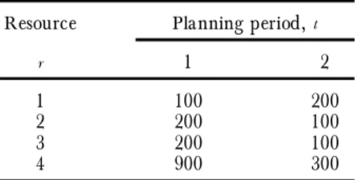
Table 4. Capacity requirements on each resource in example ( Case 1) . Resource Planning period, t
r 1 2
1 100 200
2 200 100
3 200 100
4 900 300
4. Illustrative examples
In this section we illustrate the importance of concur-rent consideration of design selection, process planning and production planning activities with some examples. Out of the many possible trade-os we shall consider only a few of them to bring out the salient points. Also, short examples are adequate for this purpose. Computation experience with large-size problems will be presented in Section 5.
E xample ( C ase 1). Let us ® rst consider only one design and one process plan for each product that corresponds to the minimum processing cost. Consider the data given in Table 3.
One design and one process plan are speci® ed for each product. The processing costs are 15 and 35 for products 1 and 2, respectively.
The capacity ( time) requirement of each type of resource can easily be computed from the demand and routing information. This is summarized in Table 4.
If we compare the available time ( Table 3) with the required processing time ( Table 4) on resources, it is obvious that resource 4 does not have enough capacity available to meet the demand completely, while resources 1, 2 and 3 have excess capacities. It can be observed that demand cannot be met even with late shipment and early production. Further, this gives rise to situations where some reources are idle while others are overloaded.
E xample ( C ase 2). Now let us consider that we can
pro-duce a dierent variation ( design) of product type 1
which is acceptable to the customer. However, this incurs a higher processing cost ( 20 per unit as compared to 15 per unit using the original design) . In addition, let there be an alternative resource 4 ( along with to resource 3) , which can create feature 1 for product 2. If this option is used the process cost increases from 35 to 40 per unit for product 2. The revised time and cost matrices, and the
late shipment and inventory holding cost
[
httÂ
(p)]
( assumed to be the same for both products) are shown in Table 5. All other data remain the same for case 1.
We solved model P0 with the revised data and the process plans obtained are shown in Table 6.
Here we notice that the lowest cost design ( design 1 of product 1) and the lowest cost process plan ( plan 2 of product 2) were not selected to meet all the demand. This could not be done because there was not enough capacity on resources, as we observed in case 1. Also, with addi-tional options ( in process plans and design variation) , a smoother workload distribution can result ( as observed from Table 7) .
Clearly this result demonstrates that there are advan-tages to considering more than one design and more than one process plan wherever available, even though
choos-ing an alternative design or process plan may increase the processing costs.
This also shows that a process plan or design with a higher processing cost can be selected by the model if it yields a lower overall cost ( sum of the late shipment cost, inventory holding cost and processing cost) .
172 G . K . A dil
Table 5. Time and cost data for example ( Case 2) Product 1 Rrf(1
,
1)[
Crf(1,
1)]
Trf(1,
2)[
Crf(1,
2)]
f f r 1 2 r 1 2 3 1 10 [5] Ð 1 10 [5] Ð Ð 4 Ð 50 [10] 2 Ð 20 [10] Ð 3 Ð Ð 10 [5] Product 2 Trf(2,
1)[
Crf(2,
1)]
f r 1 2 3 2 Ð 10 [10] ± 3 10 [15] Ð Ð 4 20 [20] Ð 20 [10] httÂ(1)= httÂ(2) tÂ
t 1 2 1 0 5 2 20 0Table 6. Process plans obtained in example ( Case 2) .
k[process plan] p d t t
Â
X(kpdttÂ
) 1[
(1,
1),
(2,
4)]
1 1 1 1 4 1[
(1,
1),
(2,
2),
(3,
3)]
1 2 2 1 6 1[
(1,
1),
(2,
4)]
1 1 2 2 6 1[
(1,
1),
(2,
2),
(3,
3)]
1 2 2 2 14 2[
(1,
3),
(2,
2),
(3,
4)]
2 1 1 1 20 2[
(1,
3),
(2,
2),
(3,
4)]
2 1 2 2 10 Table 7. Workload distributions in machines in example ( Case 2) .Resource Planning period, t
r 1 2
1 100 200
2 320 380
3 260 240
4 600 500
5. Computational experience
In this section computation experience of the column generation scheme is reported for large problems. The revised simplex algorithm incorporating the proposed column generation scheme was coded in Fortran and executed on a Sun Sparc station. Data for the test prob-lems were generated as follows ( Table 8) .
Number of product types (P), time periods (T) and
resources (R). Dierent combinations of these variables are taken ( Table 8) . The resulting basis size [given by
(P + R)
´
T ], number of designs ( Dp) and total number of resources in time ( cost) matrix,(Rpd) are also shown.Number of design features(Fpd). These are kept at two levels, 5 and 10.
Available time on resources(Brt). This is kept as 10 000 time units for each resource at each time period.
Product demand (Dpt). The values for demand are
generated from a uniform distribution between 25 and 50. However, the demand actually may not have uniform distribution. The same applies for other data generated. Cost
[
Crf(pd)]
and time[
Trf(pd)]
. These are generated from uniform distributions between 5 and 20.Late shipment and inventory costs
[
httÂ
(p)]
. These are generated from a uniform distribution between 5 and 10. A total of 10 problems are generated ( Table 8) and solved. Table 9 reports the computational experience of these problems.The number of explicit columns, the number of times the generated columns entered the basis, the number of times problem SP is solved, the number of simplex itera-tions and the CPU time are reported. The solution time appears to increase greatly with increase in the number of columns. All the problems were solved within 35 min of CPU time.
6. Discussion
Model P0, developed in Section 2, considers minimiza-tion of the sum of the processing cost, late shipment cost and inventory cost. This model illustrates the importance of considering integration of design, process plan and production planning activities. Some other objectives may also be relevant in certain situations. For instance,
there may exist dierences in the selling price of two
variations ( designs) of the same product. To model this we can de® ne S(pd) as the unit selling price of product type p produced in design d and formulate model P1.
P1: Maximize z1=
å
tå
tÂ
å
på
då
kå
få
r S(pd)X(kpdttÂ
)-
å
tå
tÂ
å
på
då
kå
få
r Arf(k pdttÂ
)´
Crf(pd)X(kpdttÂ
)-
å
tå
tÂ
å
på
då
k httÂ
(p)X(kpdttÂ
) (6) Subject to: constraints ( 2) ± ( 4) .Table 8. Problem sets tested.
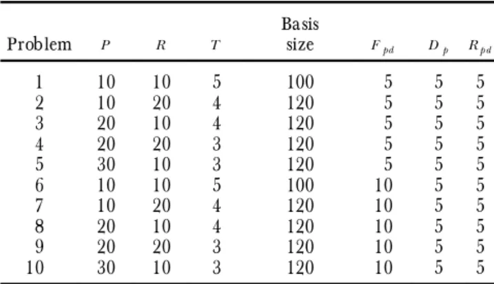
Problem P R T Basissize Fpd Dp Rpd
1 10 10 5 100 5 5 5 2 10 20 4 120 5 5 5 3 20 10 4 120 5 5 5 4 20 20 3 120 5 5 5 5 30 10 3 120 5 5 5 6 10 10 5 100 10 5 5 7 10 20 4 120 10 5 5 8 20 10 4 120 10 5 5 9 20 20 3 120 10 5 5 10 30 10 3 120 10 5 5
Table 9. Computational results
Problem Number of explicit X columns Number of times X columns entered Number of times SP solved Total number of simplex
iterations CPU time( seconds)
1 3.9´ 106 50 12 750 50 36.0 2 2.5´ 106 40 8 200 40 49.6 3 5.0´ 106 81 32 800 81 102.9 4 2.8´ 106 62 18 900 62 77.6 5 4.2´ 106 278 127 350 282 351.8 6 1.2´ 1010 140 35 750 142 110.7 7 0.8´ 1010 43 8 800 43 53.6 8 1.6´ 1010 901 360 400 901 1215.8 9 0.9´ 1010 552 166 500 554 729.0 10 1.3´ 1010 1536 691 650 1536 2112.9
The structures of model P0 and P1 are similar, and the column generation scheme developed to solve P0 can be suitably adapted for solving P1.
7. Conclusions
Product design, process planning and production plan-ning are often considered independently. However, in
order to eectively respond to the changes in business
situations, such as changes in demand forecast, product mix and technology, it becomes desirable to consider them concurrently.
We have developed a mathematical model which con-currently selects product design, generates process plans and develops production plans to minimize the sum of processing cost, late shipment cost and inventory holding cost. It has been shown that the number of process plans
can be large and therefore an e cient column generation
scheme has been developed. The model and solution pro-cedure are illustrated with examples. A problem with
over 1
´
1010 variables has been solved on a Sun Sparcstation within 35 min. A possible variation of the model is
also presented that considers the dierence in selling
price which may exist for products made in dierent
designs.
A cknowledgement
The author would like to thank the anonymous refer-ees for their suggestions.
References
Ar c e l u s, F . J ., and Sr iniv a sa n, G., 1995, On the integration of production, inventory and trade-credit policies, P roduction
P lanning & C ontrol, 6, 455± 460.
De w h u r st, P., and Bo o t h r o y d, G., 1988, Early cost
estima-tion in product design, J ournal of M anufacturing S ystem s, 7, 183± 191.
ElMa r a g h y, H. A ., and ElMa r a g h y, W . H .,1992, Bridging
the gap between process planning, production planning and control, in P roceedings of 24th C IR P International S em inar on
M anufacturing S y stems, Copenhagen, Denmark, 11± 12 June, pp. 1± 10.
Ho r v a t h, M ., Ma r k u s, A ., and Va nc z a, J ., 1996, Process planning with genetic algorithms on results of knowledge-based reasoning, International J ournal of Computer Integ rated
M anufacturing, 9, 145± 166.
Hu a ng, S. H ., Zh a ng, H. C., and Smit h, M . L ., 1995, A pro-gressive approach for the integration of process planning and scheduling, II E T ransactions, 27, 456± 464.
La r se n, N . E., and Cl a u se n, J ., 1992, Applied methods for integration of process planning and production planning and production control, M anuf acturing International, 349± 364.
Ra j a ma ni, D., Sing h, N., and Ane j a, Y. P., 1996, Design of cellular manufacturing systems, International J ournal of
P roduction R esearch, 34, 1917± 1928.
A ppendix. Illustration of column generation scheme
Consider the following problem.
P = 1;D1= 2;F11 = F12= 2;T =2;Brt = 1000
"
(r,
t);D11= D12= 30.
Processing cost and time matrices for the two designs are as follows. Design 1 Trf(1
,
1)[
Crf(1,
1)]
f r 1 2 1 20 [5] 9999 [9999] 2 9999 [9999] 50 [10] Design 2 Trf(1,
2)[
Crf(1,
2)]
f r 1 2 1 20 [5] 9999 [9999] 2 9999 [9999] 30 [15]Inventory or late shipment cost:
htt
Â
=[ ]
20 00 5Iteration 0: The size of the basis is 8. After introducing
excess variables ( e) , arti® cial variables ( a) and slacks ( s) the constraints are:
å
tå
då
k X(k,
1,
d,
t,
1)+ a1-
e1= 30å
tå
då
k X(k,
1,
d,
t,
2)+ a2-
e2= 30å
tÂ
å
då
kå
f A1,f(k,
1,
d,
1,
tÂ
)T1,f(1,
d)´
X(k,
1,
d,
1,
tÂ
)+ s3 = 1000å
tÂ
å
då
kå
f A2,f(k,
1,
d,
1,
tÂ
)T2,f(1,
d)´
X(k,
1,
d,
1,
tÂ
)+ s4 = 1000å
tÂ
å
då
kå
f A3,f(k,
1,
d,
1,
tÂ
)T3,f(1,
d)´
X(k,
1,
d,
1,
tÂ
)+ s5 = 1000 174 G . K . A dilå
tÂ
å
då
kå
f A1,f(k,
1,
d,
2,
tÂ
)T1,f(1,
d)´
X(k,
1,
d,
2,
tÂ
)+ s6= 1000å
tÂ
å
då
kå
f A2,f(k,
1,
d,
2,
tÂ
)T2,f(1,
d)´
X(k,
1,
d,
2,
tÂ
)+ s7= 1000å
tÂ
å
då
kå
f A3,f(k,
1,
d,
2,
tÂ
)T3,f(1,
d)´
X(k,
1,
d,
2,
tÂ
)+ s8= 1000 Basic variables (BV) ={
a1,
a2,
s3,
s4,
s5,
s6,
s7,
s8}
Cost vector (CV) =
{
M,
M,
0,
0,
0,
0,
0,
0}
( where M = 90 000 was taken) .Basis ( B) = identity matrix [I]
Simplex multiplier =
[
CV][
B-1]
=[
CV][
I]
=[
CV]
. Or,{
U11= U12= M,
V11= V21= V31= V12= V22= V32= 0}
Iteration 1. There are a total of 4
´
1´
2´
2´
2 = 32 explicit columns. The number of process plans ( the rangeof k) = 22 = 4 for each design. We will not enumerate
columns over k but will ® nd the one for the most
promis-ing k* by solving problem SP. For instance, consider
design d = 1.
Solving SP is equivalent to computing the following matrix and then selecting the minimum in each column.
5
-
20´
0 9999-
9999´
0 9999-
9999´
0 10-
50´
0[
]
= 5 * 9999 9999 10*[
]
In other words, for each feature ( column) ® nd the resource ( corresponding to the minimum row entry
marked by *) to de® ne the process plan k*. This gives,
U(1
,
1) = 5 + 10 = 15 for k*= 1 ( number it as 1, say) . By following a similar process, we obtain U(1,
2) = 20.Thus design d*= 1 is selected. The most promising
pro-cess plan 1 for the selected design 1 can be described by the following binary matrix:
Arf(1
,
1,
1,
t,
tÂ
) matrixf
r 1 2
1 1 0
2 0 1
The process plan can also be described as 1
[
(1,
1),
(2,
2)]
. Now we compute t*and t*Â
.F(1) = 15 + minimum [minimum{( 0± M) , ( 5± M) },
minimum {( 20± M) , ( 0± M) }] or, F(1)= 15
-
M; ( the two combinations t = 1, tÂ
= 1 and t = 2, tÂ
= 2 have a tie) .Let us pick the ® rst combination, i.e. t*= 1 and
t*
Â
= 1.The entering variable is X(1
,
1,
1,
1,
1) and entering column =[
1,
0,
20,
0,
50,
0,
0,
0]
. Iteration 2. BV ={
a1,
a2,
s3,
s4,
X(1,
1,
1,
1,
1),
s6,
s7,
s8}
CV ={
M,
M,
0,
0,
15,
0,
0,
0}
{
U11 = U12= M,
V11 = V21 = 0, V31<
0, V12 = 0, V22= V32 = 0}
Variable X(1
,
1,
1,
2,
2) enters with F(1)= 15-
M . The entering column is[
0,
1,
0,
20,
0,
50,
0,
0]
.Iteration 3.
BV =
{
a1,
a2,
s3,
s4,
X(1,
1,
1,
1,
1),
X(1,
1,
1,
2,
2),
s7,
s8}
CV =
{
M,
M,
0,
0,
15,
15,
0,
0}
{
U11 = U12= M , V11<
0,
V21<
0, V31= V12=-
M ,V22= V32 = 0
}
Variable X(2
,
1,
2,
1,
1) enters with F(1)= 20-
M . Selected process plan is 2[
(1,
1)(2,
3)]
. The entering column is[
1,
0,
20,
0,
0,
0,
30,
0]
. Iteration 4. BV ={
X(2,
1,
2,
1,
1),
a2,
s3,
s4,
X(1,
1,
1,
1,
1), X(1,
1,
1,
2,
2),
s7,
s8}
CV ={
20,
M,
0,
0,
15,
15,
0,
0}
{
U11 = 20, U12= M , V11 = V21 = 0, V31<
0, V12<
0, V22= V23 = 0}
Variable X(2
,
1,
2,
2,
2) enters with F(1)= 20-
M . The entering column is[
0,
1,
0,
20,
0,
0,
0,
30]
.Iteration 5. BV =
{
X(2,
1,
2,
1,
1),
X(2,
1,
2,
2,
2),
s3,
s4,
X(1,
1,
1,
1,
1),
X(1,
1,
1,
2,
2),
s7,
s8}
CV ={
20,
20,
0.0,
15,
15,
0,
0}
{
U11 = 20, U12= 20, V11= V21 = 0, V31<
0, V12<
0, V22= V32 = 0}
At this iteration it was found that no X -column could
enter as F(1) was equal to 0. Also, no slack or excess
variable can enter so the procedure terminates. The opti-mal solution was
k[process plan] p d t t
Â
X ( kpdttÂ
) ProcessingcostInventory/ late shipment
cost Plan cost
1
[
(1,
1),
( 2,
2)]
1 1 1 1 20 300 0 3001
[
(1,
1),
( 2,
2)]
1 1 2 2 20 300 0 3002
[
(1,
1),
( 2,
3)]
1 2 1 1 10 200 0 2002
[
(1,
1),
( 2,
3)]
1 2 2 2 10 200 0 200Total cost 1000
![Table 5. Time and cost data for example ( Case 2) Product 1 R rf ( 1 , 1 ) [ C rf ( 1 , 1 ) ] T rf ( 1 , 2 ) [ C rf ( 1 , 2 ) ] f f r 1 2 r 1 2 3 1 10 [5] Ð 1 10 [5] Ð Ð 4 Ð 50 [10] 2 Ð 20 [10] Ð 3 Ð Ð 10 [5] Product 2 T rf ( 2 , 1 ) [ C rf ( 2 , 1 ) ] f r](https://thumb-eu.123doks.com/thumbv2/9libnet/5645248.112371/7.820.424.790.81.529/table-time-cost-data-example-case-product-product.webp)