Operational approach in the weak-field measurement of polarization fluctuations

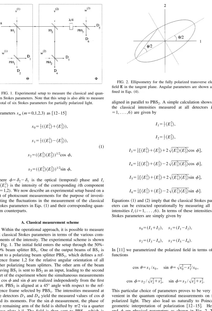
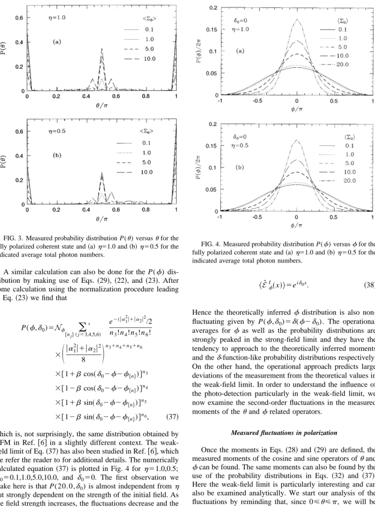
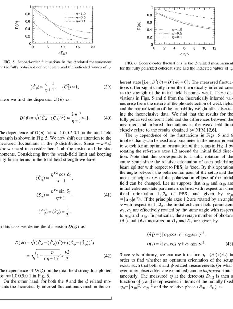
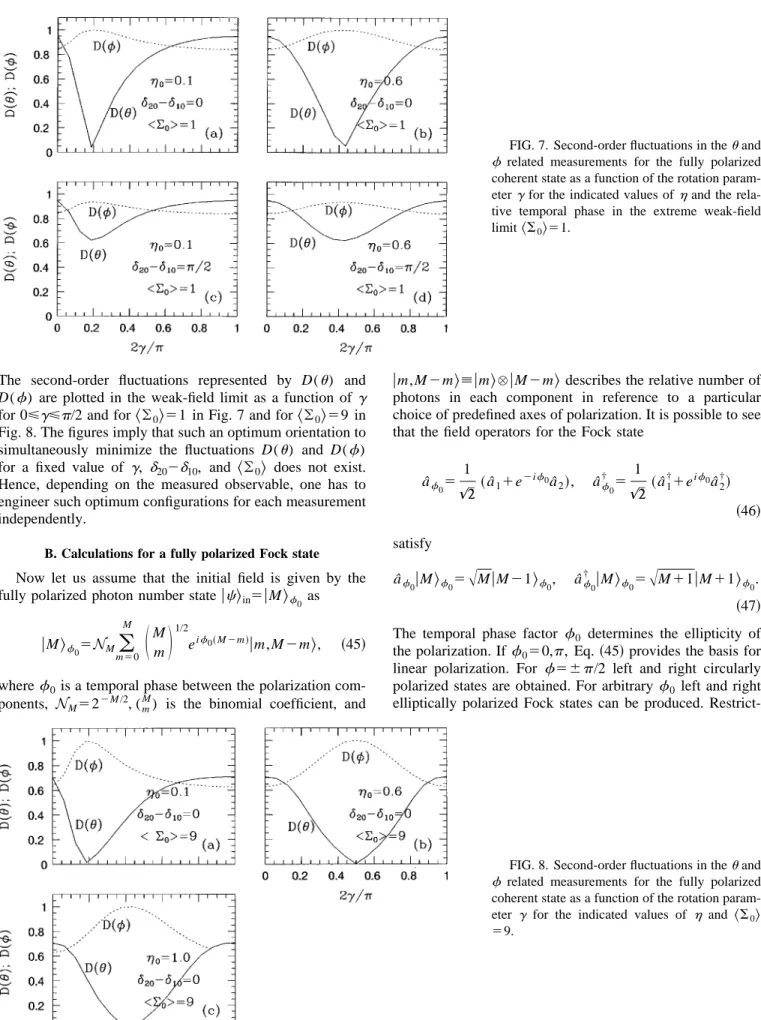
Operational approach in the weak-field measurement of polarization fluctuations

T. Hakiog˘lu

Physics Department, Bilkent University, 06533-Ankara, Turkey ~Received 1 July 1998!

The operational approach to the measurement of phase studied by Noh, Fougere`s, and Mandel@Phys. Rev.

A 45, 424~1992!; 46, 2840 ~1992!; Phys. Rev. Lett. 71, 2579 ~1993!; Phys. Rev. A 47, 4535 ~1993!# is applied

to the measurement of the state of polarization of fully polarized light. Operational counterparts of the quantum Stokes parameters are introduced and their fluctuations are examined. It is shown that if the polarized field is weak, the measured fluctuations are influenced not only by the quantum properties of the source field but also that of the measurement. This character is reflected on the measured probability distributions of the parameters of polarization, which are also investigated independently for the fully polarized coherent states and the Fock states as the initial field strength is varied. Finally, connection between the operational approach to the

measurement of polarization and the su~2! interferometry is examined. @S1050-2947~99!01402-X#

PACS number~s!: 42.50.Dv, 85.60.Gz

I. INTRODUCTION

The idea of the operational approach as an experimental technique based on photon counting in the measurement of quantum-phase fluctuations was suggested in 1986 by Bar-nett and Pegg@1# in the context of a measured phase operator using certain homodyne experiments and more recently was formulated in detail by Noh, Fouge`res, and Mandel ~NFM! @2#. The operational phase measurement is based on using N-port quantum homodyne detectors of which the analogy with classical homodyne approach is based on the purpose of extracting information about the phase between two initial fields by performing a complete set of photocount measure-ments between the components of the field. This procedure of obtaining the phase information between two fields de-pends on the particular experimental scheme through its clas-sical analogy of relating the relative photocount measure-ments to certain cosine and sine functions of the relative phase. Since, through this suggested analogy, different quan-tum measurement schemes would correspond to different classical ones, the information extracted for the relative phase is expected to be different for different experimental schemes. Indeed, this point has been demonstrated in the formulation of the operational phase measurement by NFM by starting with two different classical and quantum mea-surement schemes where one meamea-surement used two-port homodyne detection whereas the second one used four-port homodyne detection@2,3#. The two-port measurement yields either the cosine or the sine information about the phase failing to give the full phase information. In the four-port scheme the simultaneous measurements were made possible by well-defined trigonometric operators of the relative phase where the full information on the phase and its fluctuations can be extracted. On the other hand, a comparison of NFM’s operational approach with the operational approach intro-duced by Vogel and Schleich @4# has been compared by Lynch @5#, who found agreement between the two opera-tional schemes.

Another particularly important part of this scheme depen-dence manifests itself in the weak-field measurements in which the quantized nature of light as well as that of the

detectors becomes crucial when the homodyne detectors have a relatively high probability of registering a few or null photocounts within the measurement time interval T. This being the case for a single set of measurements, one consid-ers an ensemble of repeated measurements under the same initial conditions. There, each repeated measurement would have generally different but equally acceptable configura-tions of detected photons and one has to make a distinction between the outcome of a single measurement from the av-erage outcome of a collection of such repeated measurements under otherwise the same conditions. Despite the fact that the experimental verification of NFM’s operational approach was successfully made by the same group@6#, the appearance of the discrete outcomes in the phase measurements in their scheme was subject to long and heavy discussions@7–10#. In this work we suggest another application of their approach to the operational measurement of the state of polarization of a fully polarized source. In an earlier publication @11# we in-vestigated a particular extension of NFM’s operational ap-proach to the measurement of the Stokes parameters of a fully polarized weak coherent light. In this work we will extend this formalism introduced in @11# to a more general framework by including the calculations for the measured probability distributions of the polarization fluctuations and also examine the case thoroughly when the initial field is a fully polarized Fock state.

We start with a brief outline of the operational approach to the measurement of polarization fluctuations when the po-larized field is given in a classical as well as a quantum state. In Sec. II we present the general formalism of calculating the polarization fluctuations and their corresponding probability distributions. Sections II A and II B are devoted to the spe-cific calculations corresponding to two different fully polar-ized initial quantum states of the field as coherent and Fock states, respectively. Section II C is devoted to the connec-tions between the operational approach and the su~2! inter-ferometry.

Classically, the state of polarization of a fully polarized monochromatic field Ei5eicos(vt1di), where i51,2 are the

polarization indices of two preselected orthogonal polariza tion eigenmodes, can be manifestly described by four Stokes PRA 59

parameters sm(m50,1,2,3) as @12–15# s0512~

^

E1 2

_&

₁

_^

_E 2 2

_&

_!, s15 1 2~

^

E1 2

_&

₂

_^

E₂2

&

!, ~1! s₂5~

^

E₁2

&^

E₂2

&

!1/2_cosf,

s35~

^

E1 2

_&^

_E

2

2

_&

_!1/2_{sin f,}

where f5d22d1 is the optical ~temporal! phase and Ii

5

^

E_i2

&

is the intensity of the corresponding ith component (i51,2). We now describe an experimental setup based on a set of photocount measurements for the purpose of investi-gating the fluctuations in the measurement of the classical Stokes parameters in Eqs.~1! and their corresponding quan-tum counterparts.

A. Classical measurement scheme

Within the operational approach, it is possible to measure all classical Stokes parameters in terms of the various com-ponents of the intensity. The experimental scheme is shown in Fig. 1. The initial field enters the setup through the 50%-50% beam splitter BS1. One of the output beams of BS1 is

sent to a polarizing beam splitter PBS1, which defines a

ref-erence frame 1,2 for the relative angular orientation of all other polarizing beam splitters. The other arm of the beam leaving BS1is sent to BS2as an input, leading to the second

part of the experiment where the simultaneous measurements of cosfand sinf are realized independently from the first part. PBS2 is aligned at a 45° angle with respect to the

ref-erence frame selected by PBS1. The intensities measured at

the detectors D3 and D4 yield the measured values of cosf

and its moments. For the sinf measurement, the phase of the remaining arm of the field is shifted byp/2 via a quarter wave plate l/4. The field is then sent to PBS3, which is

aligned in parallel to PBS2. A simple calculation shows that

the classical intensities measured at all detectors Di(i

51, . . . ,6) are given by I1512

^

E1 2

_&

_, I₂51 2

^

E2 2

_&

_, I35 1 4@

^

E1 2

_&

₁

_^

E₂2

&

12

A

^

E2₁

&^

E₂2

&

cosf#,

~2! I45

1 4@

^

E1

2

_&

₁

_^

E₂2

&

22

A

^

E2₁

&^

E₂2

&

cosf#, I55 1 4@

^

E1 2

_&

₁

_^

_E 2 2

_&

₁₂

A

_^

_E 1 2

_&^

_E 2 2

_&

_sinf#, I65 1 4@

^

E1 2

_&

₁

_^

E2 2

_&

₂₂

A

_^

E1 2

_&^

E2 2

_&

sinf#.

Equations~1! and ~2! imply that the classical Stokes param-eters can be extracted operationally by measuring all field intensities Ii(i51, . . . ,6). In terms of these intensities, the

Stokes parameters are simply given by

s05~I11I2!, s15~I12I2!,

~3! s25~I32I4!, s35~I52I6!.

In @11# we parametrized the polarized field in terms of the functions cosu5s₁/s₀, sinu5

A

s₀22s₁2/s₀, ~4! cosf5s2/

A

s2 2_1s 3 2 , sin f5s3/

A

s2 2_1s 3 2 .

This particular choice of parameters proves to be very con-venient in the quantum operational measurements on fully polarized light. They also lead us naturally to Poincare´’s geometric interpretation of polarization @12–15#. Here u and f are physical parameters as shown in Fig. 2. Their FIG. 1. Experimental setup to measure the classical and

quan-tum Stokes parameters. Note that this setup is also able to measure a total of six Stokes parameters for partially polarized light.

FIG. 2. Ellipsometry for the fully polarized transverse electric field E in the tangent plane. Angular parameters are shown as

values are directly connected with the ellipsometry of the polarized field. From now on we will adopt this parametri-zation and study the polariparametri-zation fluctuations in terms of the fluctuations of these observables.

B. Quantum measurement scheme

The classical description above is adequate when the field intensity is sufficiently high. The vacuum fields, which are not present in the classical approach, are necessary for the correct quantum description of the apparatus as well as the field observables.

In Fig. 1 the field operators dˆ₁,dˆ₂ at the output of PBS₁ are related to the input field components aˆ1,aˆ2 as@11#

dˆ15

1

& ~raˆ11tvˆ1~1!!, dˆ25

1

&~raˆ21tvˆ2~1!!, ~5!

where r5i/& and t51/& are the field reflection and trans-mission coefficients and vˆj

(1)

( j51,2) are the polarized vacuum fields entering through the vacuum port of BS1. If

the measurement scheme in Fig. 1 is extended to include the photodetectors Di(i53,4,5,6), thenfmeasurements can be

made compatible with a proper quantum treatment of all fields. The output fields of PBS2and PBS3at D3,D4,D5,D6

are given by dˆ35 1 & @~traˆ11r 2 vˆ1~1!1tvˆ1~2!!1~traˆ21r2vˆ2~1!1tvˆ2~2!!#, dˆ₄51

& @2~traˆ11r2vˆ1~1!1tvˆ1~2!!1~traˆ21r2vˆ2~1!1tvˆ2~2!!#,

~6! dˆ55 1 & @i~t 2_aˆ 11trvˆ1~1!1rvˆ1~2!!1~t 2_aˆ 21trvˆ2~1!1rvˆ2~2!!#, dˆ65 1 & @2i~t 2_aˆ 11trvˆ1~1!1rvˆ1~2!!1~t 2_aˆ 21trvˆ2~1!1rvˆ~2!2 !#.

In connection with their classical counterparts in Eqs.~3!, we are now at a point to suggest the quantum Stokes parameters for the field operators dˆiwithin this operational approach in

terms of the observable photon number operators nˆi5dˆi †

dˆias

Sˆ05nˆ11nˆ2, Sˆ15nˆ12nˆ2,

~7! Sˆ25nˆ32nˆ4, Sˆ35nˆ52nˆ6.

In Eqs.~6! all field operators commute as a manifestation of the vacuum fields. Hence, in Eqs. ~7! we have @Sˆi,Sˆj#50

(iÞ j) and all photon number operators can be simulta-neously measured at the detectors Di(i51, . . . ,6). As a

result, Eqs. ~7! are compatible with their classical counter-parts in Eqs. ~3!. This property of the Sˆi(i50, . . . ,3)

op-erators allows us to further suggest an extension~4! to their operator counterparts as Cˆ_u5Sˆ₀21Sˆ1, Sˆu5~12Cˆ_u 2_!1/2_, ~8! Cˆ_f5Sˆ2~Sˆ2 2_1Sˆ 3 2_!21/2 , Sˆ_f5Sˆ3~Sˆ2 2_1Sˆ 3 2_!21/2 . Cˆ_u,Sˆ_uand Cˆ_f,Sˆ_fare well-defined and compatible quantum observables. They commute with each other and satisfy the operator relations Cˆ_u21Sˆ_u251 and Cˆ_f21Sˆ_f251 and, as a re-sult, can be measured simultaneously.

One of the benefits of adopting Eqs.~7! and ~8! is that all measurements are now based on pure photon counting de-pending on the measured photocounts at the detectors Di(i

51, . . . ,6) and hence they do not involve any temporal in-terference effects. This is an advantage of the operational measurement, which will be transparent later in our discus-sion of the weak-field limit.

Equations ~8!, hereinafter referred to as the operational quantum Stokes parameters ~OQSP!, are the most conve-nient choice forSˆi(i50, . . . ,3) befitting the purpose of the

photocount measurement scheme of Fig. 1. All operators in Eqs. ~8! are now compatible with the classical variables of Eqs. ~4! as long as the measurements of the Sˆ2 andSˆ3

op-erators do not yield zero simultaneously.

II. MEASUREMENT OF POLARIZATION FLUCTUATIONS IN WEAK FIELDS

The operational approach as applied to the polarization measurement of a fully polarized and weak initial field is based on individual detections of single photons where the quantum nature of the field as well as that of the detection mechanisms is dominant. The influence of the direct quan-tum homodyne detection on the statistics of a quanquan-tum mea-surement has been examined by Mandel @16#, Kelley and Kleiner@17#, and Glauber @18# and expressed in the form of a combined quantum probability distribution

P~$nj%!5

)

j51 N :~dˆ†_jdˆj!njexp~2dˆj †_dˆ j!/nj!:, ~9!

where : : accounts for the normal ordering of the operators dˆ_i†,dˆ_i inside and dˆ_i†dˆ_i corresponds to the photon number operator. Throughout the calculations the measurement time interval will be assumed to be much smaller than the coher-ence time ~which is naturally satisfied for a monochromatic field! and much larger than the inverse of the oscillation frequency of the field. Under these conditions it is possible to consider the simplest case when the photocount measure-ment at the detectors is time translationally invariant and linearly dependent on the measurement time interval T.

Including the quantum effects of the homodyne detection in Eq. ~9!, an individual measurement of an arbitrary field operator f ($nˆj%) yields the measured value

^

f~$nˆj%!

&

5N

(

$n_j%

f~$nj%!TrˆrˆP~$nj%!‰, ~10!

where the trace is considered over the complete set of states in the density matrix of the initial fieldrˆ5uc

&

in in

^

cu. With

Eqs.~9! and ~10! representing a general scheme of measure-ment in the operational approach, we now consider for f ($nˆj%) the operators of$nˆj%( j51,2 or 3,4,5,6!,

Eˆu~x!5~Cˆu1iSˆu!x, Eˆf~x!5~Cˆf1iSˆf!x for xPR.

~11! In the construction of Cˆ_u,Sˆ_u and Cˆ_f,Sˆ_f pairs in Eqs.~8!, the compatibility conditions@Sˆi,Sˆj#50 of the OQSP ensure

thatiEˆ_u(x)i51 and iEˆ_f(x)i51; hence Eˆ_u(x) andEˆ_f(x) are unitary operators for all xPR. According to the procedure outlined in the context of Eqs. ~9! and ~10!, the measure-ments of these operators yield

^

Eˆu~x!

&

5Nu

(

$n_j%

F

n12n212i

A

n1n2 n₁1n₂

G

x

^

P~$nj%!

&

~12! and

^

Eˆf~x!

&

5Nf

(

$n_j%

F

~n32n4!1i~n52n6!

A

~n32n4!21~n52n6!2

G

x

^

P~$nj%!

&

, ~13! where

^

P($nj%)

&

5Trˆuc

&

in in

^

cuP($nj%)‰. In Eq. ~12! $nj%

5(n1,n2) and in Eq. ~13! $nj%5(n3,n4,n5,n6). Clearly,

Eq.~12! is well defined if n1,n2are not simultaneously zero

and similarly Eq. ~13! is well defined if n32n4 and n52n6

are not simultaneously zero in the respective summations above. The idea of the elimination of the configurations n1

5n250, and n35n4 and n55n6 from the statistical weight

has been introduced as a crucial element of the operational approach @2,3,6,9# in the implementation of the statistical averages. The effective weight of such configurations be-comes non-negligible particularly in the case when the initial field strength is sufficiently weak when the probability of receiving zero photons within the detector’s measurement time interval T is finite. For instance, the weight of observing zero photons simultaneously at the detectors D1,D2 is given

by^P~0,0!&. The result of such a null measurement is incon-clusive in the calculation of the averages in Eq.~12!. Simi-larly, n35n4 and n55n6 yield additional inconclusive

re-sults in the measurement on

^

Eˆ_f(x)

&

in Eq. ~13!. The measured averages are then normalized by excluding the to-tal statistical weight of these inconclusive configurations from the integrated probability. For strong fields, the weight of such ambiguous outcomes is smaller and in the classical field limit there is no contribution from such terms, viz., Nu5Nf51. In the measurement of the temporal phase the

individual fluctuations of these weak components as well as the fluctuations in the relative number of photons can be strong due to the absence of a classical reference source~i.e., a strong local oscillator!. Hence the normalization technique introduced by NFM proves to be essential for any opera-tional measurement based on phase and thus also for our approach here.

More explicitly, this normalization procedure amounts to @2#

N_u21₅₁₂

_^

_P~0,0!

_&

_~14!

and

Nf21512

(

n,m

^

P~n35n45n,n55n65m!

&

~15!

in Eqs. ~12! and ~13!. The observed unitarity conditions of Eˆu(x) and Eˆf(x) suggest that one can associate a classical

random variable eixuand eixfrespecting the probability dis-tributions P(u) and P(f) such that@6#

^

Eˆu~x!

&

5

E

0 p du eixuP~u!,

^

Eˆ_f~x!

&

5

E

2p p df eixfP~f!. ~16! The probability distributions can then be obtained by the inverse Fourier transformations of Eq.~16! by

P~u!5

E

2`

` dx

2p e

2ixu_$

_^

_Eˆ

u~x!

&

1

^

Eˆu~2x!

&

%,

~17! P~f!5

E

2` ` dx 2p e 2ixf

_^

_Eˆ f~x!

&

, with*0pduP(u)5*2pp dfP(f)51.

Defining two auxiliary functions of$n%j by

u$n_%5tan21

S

2

A

n1n2 n12n2

D

, f_$n_%5tan21

S

n52n6 n32n4

D

, ~18!

where $n%5(n1,n2) and $n%5(n3,n4,n5,n6) for u and f

respectively, and using Eqs.~12! and ~13!, the moments for a generalized initial state uc

&

inread

^

Eˆu~x!

&

5Nu

(

8

n₁,n₂ eixu_$n%

_^

_P~$n j%!

&

where

^

P~$nj%!

&

5Nu

(

8

n₁,n₂

F

~n12n2!1i2

A

n1n2 n11n2

G

x 3₂n_11n21_n 1!n2! in

^

cu:~aˆ1 † aˆ1!n1~aˆ2 † aˆ2!n2 3exp@21/2~aˆ1 †_aˆ 11aˆ2 †_aˆ 2!#:uc

&

in, ~19! and

^

Eˆf~x;d0!

&

5Nf

(

8

n₃,n₄,n₅,n₆ eixf$n%

^

P~$nj%,d0!

&

where

#P~$n_j%,d₀! 5Nf

(

8

n₃,n₄,n₅,n₆

F

~n32n4!1i~n52n6!

A

~n32n4!21~n52n6!2

G

x 3₈n₃1n₄1n₅1n₆1_n 3!n4!n5!n6! 3in

^

cu:~aˆ1 †_1aˆ 2 †_!n_6~aˆ 11aˆ2!n3~2aˆ1 †_1aˆ 2 †_!n₄

3~2aˆ11aˆ2!n4~2iaˆ1 †_1aˆ 2 †_!n_5~iaˆ 11aˆ2!n5 3~iaˆ1 †_1aˆ 2 †_!n_6~2iaˆ 11aˆ2!n6 3exp@21/2~aˆ1 †_aˆ 11aˆ2 †_aˆ 2!#:uc

&

in, ~20!

withd05d22d1implicitly described in Eq.~20! as the

rela-tive temporal phase between the components of the initial field. The primes on the summations in Eqs. ~19! and ~20! now indicate that the summations are performed by exclud-ing those configurations for which the outcome is inconclu-sive.

All moments are now determined once the initial compo-nents

^

nˆ1

&

,

^

nˆ2

&

and the relative temporal phase d0 of the

inclusive fields aˆ1,aˆ2are known. In our calculations the

ini-tial field parameters are chosen as the ratio of the photon numbers h5

^

nˆ₁

&

/

^

nˆ₂

&

, the total number of photons

^

Sˆ₀

&

5

^

nˆ1

&

1

^

nˆ2

&

, and the relative temporal phased0.

The credibility of the results obtained from the quantum operational approach crucially depends on the understanding of the influence of the quantum detectors on the final statis-tics. As pointed out in Refs. @2, 3, 6, 9#, another essential element of the operational approach is the construction of an ensemble from a long series of such single operational mea-surements. The final physical results are then obtained by averaging the outcomes of single measurements over the cre-ated ensemble. Based on this prescription, we must now con-struct a physical ensemble of measured configurations in the calculations of the moments as well as the probability distri-butions in Eqs. ~19! and ~20!. The response of the quantum detectors to the incoming photons in the creation of the pho-tocurrent is a random process that obeys the Poisson statis-tics in Eq. ~9! @19#. As the photoelectrons are emitted at random times respecting this statistics, the information re-garding the initial temporal phase d0 of the incoming

pho-tons is modified and each repeated measurement is equiva-lent to superposing a random phase shiftD ond0. Hence the

process of repeated measurements creates an ensemble of temporal phase configurations d01D, with D being

uni-formly distributed over the available range. Since we con-sider in our calculations that the measurement time interval T is considerably larger than the coherence time, the available range for D is the entire 2p range. Hence the average over the created ensemble corresponds to an averaging over a uni-form distribution of D. It is clear from Eq. ~19! that the moments

^

Eˆ_u(x)

&

are independent fromd₀; hence they will also be independent of D. This implies that a uniform aver-age over D does not influence the measured moments

^

Eˆu(x)

&

and the probability distribution for P(u) is given by

P~u!5

E

2`

` dx

2p e

2ixu_$

_^

_Eˆ

u~x!

&

1

^

Eˆu~2x!

&

%, 0<u<p.

~21! On the other hand, the moments

^

Eˆ_f(x)

&

depend on the tem-poral phase d₀ and before theD average, thed₀ dependence must be replaced byd01D. This produces, at each

measure-ment, the conditioned f moments

^

Eˆ_f(x;d01D)

&

and,

fol-lowing Ref. @6#, their conditional probability distribution P(f,d0;D) is given by P~f,d0;D!5

E

2` ` dx 2p

^

Eˆf~x;d01D!

&

e 2ix~f2D!_, ~22! 2p<f<p.

Therefore, the ensemble-averaged probability distribution is

P~f,d0!5

E

2p

p dD

2p P~f;d0;D!. ~23! After a short calculation using Eqs. ~19! and ~20! in Eqs. ~21!–~23!, the probability distributions P(u) and P(f,d0)

can be expressed by P~u!5N_u

(

$n_j%d~u2u$n%!

^

P~$ nj%!

&

~24! and P~f,d0!5Nf

(

$n_j%

^

P~$ nj%,d02f$n%1f!

&

, ~25!

where the last term in Eq.~25! is obtained by using Eqs. ~20! in Eq.~22!.

On the other hand, the detectors’ influence on the mea-sured statistics can only be understood if the meamea-sured mo-ments and probability distributions are compared with those without the detectors’ influence. For this purpose and, fol-lowing Refs.@2,3#, we define the theoretically inferred values of theu andfmoments as

^

Eˆ_uI(x)

&

and

^

Eˆ_fI(x)

&

, where

^

Eˆ_uI_~x!

_&

₅ in

K

c

U

:

F

nˆ12nˆ21i2

A

nˆ1nˆ2 nˆ₁1nˆ₂

G

x :

U

c

L

in ~26! and

^

EˆfI~x!

&

5in

K

c

U

:

F

~nˆ32nˆ4!1i~nˆ52nˆ6!

A

~nˆ32nˆ4!21~nˆ52nˆ6!2

G

x :

U

c

L

in , ~27! where : : stands for the normal ordering of the field and vacuum operators inside.

We calculate the probability distributions P(u), where 0 <u<p, and P(f,d0), where2p<f<p, numerically

us-ing Eqs. ~24! and ~25!. Since cosu is single valued in theu range considered, we will only need to examine the

fluctua-tions in the Cˆ_u operator. On the other hand, in the frange considered both Cˆ_f and Sˆ_f operators will be necessary. In our calculations, the summations over an infinite range of $n%j’s are truncated at$n%j

max_{520 for all j that naturally}

re-strict the accuracy of the results to sufficiently weak initial fields. The measured moments and the probability distribu-tions are then compared with the theoretically inferred ones by using Eqs.~26! and ~27!.

A. Calculations for a fully polarized quantum coherent field

Let us now assume that the initial field is in a fully polar-ized quantum coherent stateuc

&

in5ua1,a2

&

, with the

param-eters given by a_j5ua_jueid_{j, where ua}

ju2 anddj( j51,2) are

the average number of photons and the coherent temporal phase of the jth component, respectively. The relative tem-poral phase is given, as before, by d05d22d1. From Eqs.

~19! and ~20!, the measured moments in this state are given by

^

Eˆu~x!

&

5Nu

(

8

n₁,n₂

F

~n12n2!1i2

A

n1n2 n₁1n₂

G

x 3ua1u2n1ua2u2n2 3exp$21 2~ua1u 2_1ua 2u 2_!%/2n_11n2n 1!n2! ~28! and

^

Eˆf~x;d0!

&

5Nf

(

8

$n%

F

~n32n4!1i~n52n6!

A

~n32n4!21~n52n6!2

G

x 3ua11a2u2n3u2a11a2u2n4u 2ia11a2u2n5uia11a2u2n6 3exp$21 2~ua1u21ua2u2!%/8n31n41n51n6 3n3!n4!n5!n6!, ~29!

where$n%5(n₃,n₄,n₅,n₆). For the specific initial polarized coherent state considered, using Eqs.~14! and ~15!, the nor-malizations are given by

N _u21_512exp$21 2~ua1u

2_1ua 2u

2_{!% ~30!}

and definingb52ua1uua2u/(ua1u21ua2u2), whereb<1,

N_f21₅₁₂

(

n,m

S

ua1u21ua2u2 8

D

2~n1m! 3exp$2 1 2~ua1u1ua2u2!% ~n!!2_~m!!2 3@12b2 _cos2 _d 0#n@12b2 sin2 d0#m. ~31!

We will first examine the P(u) distribution. Using Eq.~24!, the calculation of P(u) yields

P~u!5N_u

(

8

n₁,n₂ d~u2u$n%! ua1u 2n_1uga 2u 2n₂ 2n11n2_n 1!n2! 3exp$21 2~ua1u21ua2u2!% ~32!

whereu_$n%is defined by the first expression in Eqs.~18!. For

sufficiently weak fields, i.e.,

^

S0

&

!1, each detector

mea-sures null or a very few number of photons. This implies that in Eq. ~32! it is sufficient to restrict the summation over $n1,n2% to a few terms. For instance, let us consider

$n1,n2%50,1. Then including only the first-order terms in the

average total photon number, Eq.~32! can be approximately expressed in the weak-field limit by Pw(u) in the form

Pw~u!5Nw

^

S0

&

H

1 11h21d~u!1 1 11h d~u2p!

J

, ~33! where

^

S0

&

5(ua1u21ua2u2)/2 is the total average photon

number deduced from the measurements at the detectors D1,D2,h5ua1u2/ua2u2, and Nw5

^

S0

&

21 so that

*0pdu P(u)51. From Eq. ~33! we find that

^

cosu

&

w[

E

0 p du~cos u!P~u!5h21 h11,

^

cos2u

&

w51. ~34! Clearly,

^

cosu

&

win Eq. ~34! is consistent with the

theoreti-cally inferred values calculated from Eq. ~26! @i.e.,

^

cosu

&

w

5

^

Cˆ_uI

&

]. In the initial polarized coherent state the theoreti-cally inferred moments are given by

^

EˆI_u~x!

_&

₅

F

h211i2h 1/2

h11

G

x

5eix tan212Ah/~h21!_{, ~35!}

which respect a nonfluctuating distribution. Equation ~35! is also consistent with the classical calculations using Eq. ~4!. However, for the second moments we obtain

^

~CˆuI!2

&

5

S

h

21 h11

D

2

Þ

^

cos2 u

&

w. ~36!

The u distribution in Eq. ~32! is plotted in Fig. 3 for h 51.0,0.5 and

^

Sˆ0

&

50.1,1.0,5.0,10.0. The first observation in

Fig. 3~a! is that ath51.0 the probability distribution is sym-metrically centered around u5p/2. In the weak-field limit P(u) is peaked at u50,p. As the field strength is suffi-ciently increased, the central peak at u5p/2 gradually de-velops as all other peaks are suppressed. The average of cosuwithin the full range 0<u<p is zero, as it would also be expected from the theoretically inferred moments in Eq. ~35!. For hÞ1, the measured P(u) is plotted in Fig. 3~b!. The d functions in Eq. ~32! are numerically simulated by sharp Lorentzians, hence they acquire a finite width in Figs. 3~a! and 3~b!. On the other hand, using Eq. ~21!, the inferred probability distribution PI(u) can be found as PI(u)5d„u 2cos21_{(h21)/(h11)….}

A similar calculation can also be done for the P(f) dis-tribution by making use of Eqs. ~29!, ~22!, and ~23!. After some calculation using the normalization procedure leading to Eq.~23! we find that

P~f,d0!5Nf

(

8

$n_j%~ j53,4,5,6! e2~ua1 2_u1ua 2u2_/2 n3!n4!n5!n6! 3

S

ua1 2_u1ua 2u 2 8

D

n₃1n₄1n₅1n₆ 3@11b cos~d₀2f2f_$n%!#n₃ 3@12b cos~d02f2f$n%!#n4 3@11b sin~d₀2f2f_$n%!#n₅ 3@12b sin~d02f2f$n%!#n6, ~37!

which is, not surprisingly, the same distribution obtained by NFM in Ref. @6# in a slightly different context. The weak-field limit of Eq.~37! has also been studied in Ref. @6#, which we refer the reader to for additional details. The numerically calculated equation~37! is plotted in Fig. 4 for h51.0,0.5; S050.1,1.0,5.0,10.0, and d050. The first observation we

make here is that P(20.0,d0) is almost independent fromh

but strongly dependent on the strength of the initial field. As the field strength increases, the fluctuations decrease and the distribution becomes gradually narrower. On the other hand, using Eq.~27!, the theoretically inferred moments are calculated as

^

Eˆ_fI_~x!

_&

_5eid₀x_{. ~38!}

Hence the theoretically inferred f distribution is also non-fluctuating given by P(f,d0)5d(f2d0). The operational

averages for f as well as the probability distributions are strongly peaked in the strong-field limit and they have the tendency to approach to the theoretically inferred moments and thed-function-like probability distributions respectively. On the other hand, the operational approach predicts large deviations of the measurement from the theoretical values in the weak-field limit. In order to understand the influence of the photo-detection particularly in the weak-field limit, we now examine the second-order fluctuations in the measured moments of theu andfrelated operators.

Measured fluctuations in polarization

Once the moments in Eqs. ~28! and ~29! are defined, the measured moments of the cosine and sine operators ofuand fcan be found. The same moments can also be found by the use of the probability distributions in Eqs. ~32! and ~37!. Here the weak-field limit is particularly interesting and can also be examined analytically. We start our analysis of the fluctuations by reminding that, since 0<u<p, we will be confined to the measured fluctuations in the Cˆ_u operator. In the weak-field limit ~keeping only the leading term in the total field strength!

FIG. 3. Measured probability distribution P(u) versus u for the

fully polarized coherent state and~a!h51.0 and ~b!h50.5 for the

indicated average total photon numbers.

FIG. 4. Measured probability distribution P(f) versus f for the

fully polarized coherent state and~a!h51.0 and ~b!h50.5 for the

^

Cˆ_u

&

.h21

h11,

^

Cˆu2

&

.1, ~39!

where we find the dispersion D(u) as

D~u!5

A

_Š~Cˆu2

^

Cˆ_u

&

!2_{‹ .}2h 1/2

h11 <1. ~40! The dependence of D(u) forh51.0,0.5,0.1 on the total field strength is shown in Fig. 5. We now shift our attention to the measured fluctuations in the f distribution. Since 2p<f <p we need to consider here both the cosine and the sine moments. Considering first the weak-field limit and keeping only linear terms in the total field strength we have

^

Cˆ_f

&

.h 1/2_cosd 0 h11 ,

^

Sˆ_f

&

.h 1/2_sind 0 h11 , ~41!

^

Cˆ_f2

&

5

^

Sˆ_f2

&

51 2. In this case we define the dispersion D(f) as

D~f!5

A

_Š~Cˆf2

^

Cˆ_f

&

!2_‹1Š~Sˆ f2

^

Sˆf

&

!2‹ 5

A

12 h ~h11!2> ) 2 . ~42!

The dependence of D(f) on the total field strength is plotted for h51.0,0.5,0.1 in Fig. 6.

On the other hand, for both the u and the frelated mo-ments the theoretically inferred fluctuations vanish in the

co-herent state@i.e., DI(u)5DI(f)50]. The measured fluctua-tions differ significantly from the theoretically inferred ones as the strength of the initial field becomes weak. These de-viations in Figs. 5 and 6 from the theoretically inferred val-ues arise from the nature of the photodetection of weak fields and the normalization of the probability weight after discard-ing the inconclusive data. We find that the results for the fully polarized coherent field and the differences between the measured and inferred fluctuations in the weak-field limit closely relate to the results obtained by NFM @2,6#.

The h dependence of the fluctuations in Figs. 5 and 6 implies thathcan be used as a parameter in the measurement to search for an optimum orientation of the setup in Fig. 1 by rotating the reference axes 1,2 around the initial field direc-tion. Note that this corresponds to a solid rotation of the entire setup since the relative orientation of each polarizing beam splitter with respect to PBS1is fixed. By this operation

the angle between the polarization axes of the setup and the mean principle axes of the polarization ellipse of the initial field can be changed. Let us suppose that a10 anda20 are

initial coherent state parameters defined with respect to some fixed orientation 1₀,2₀ of PBS₁ and given by a_j0 5uaj 0ueidj0. If the principle axes 1,2 are rotated by an angle

g with respect to 1₀,2₀, the initial coherent field parameters a1,a2are effectively rotated by the same angle with respect

toa10anda20. In particular, the average number of photons

^

nˆ1

&

and

^

nˆ2

&

measured at D1 and D2 are given by

^

nˆ₁

&

51 2ua10cosg2a20singu 2_,

^

nˆ2

&

5 1 2ua20cosg1a10singu2. ~43!

Since g is arbitrary, we can use it to tune h5

^

nˆ1

&

/

^

nˆ2

&

in

order to find whether an optimum orientation of the setup exists such that bothuandfrelated measurements~or what-ever other observables are examined! can be improved simul-taneously. The measured h at the detectors D1,2 is then a

function ofgand is represented in terms of the initially fixed h05ua10u2/ua20u2 and the relative phase (d202d10) as

h~g!5~

A

h02tang!

2₁

A

_h

0tang sin2~d202d10!/2

~

A

h01tang!22

A

h0tang sin2~d202d10!/2

. ~44!

FIG. 5. Second-order fluctuations in theu related measurement

for the fully polarized coherent state and the indicated values ofh.

FIG. 6. Second-order fluctuations in thef related measurement

The second-order fluctuations represented by D(u) and D(f) are plotted in the weak-field limit as a function ofg for 0<g<p/2 and for

^

(₀

&

51 in Fig. 7 and for

^

(₀

&

59 in Fig. 8. The figures imply that such an optimum orientation to simultaneously minimize the fluctuations D(u) and D(f) for a fixed value of g, d202d10, and

^

(0

&

does not exist.

Hence, depending on the measured observable, one has to engineer such optimum configurations for each measurement independently.

B. Calculations for a fully polarized Fock state

Now let us assume that the initial field is given by the fully polarized photon number stateuc

&

in5uM

&

f₀ as

uM

&

f05NM_m

(

₅₀ M

S

M m

D

1/2 eif0~M2m!um,M2m

&

_, ~45! wheref0is a temporal phase between the polarization

com-ponents, NM522M/2, (m

M_{) is the binomial coefficient, and}

um,M2m

&

[um

&

^uM2m

&

describes the relative number of photons in each component in reference to a particular choice of predefined axes of polarization. It is possible to see that the field operators for the Fock state

aˆ_f 05 1 & ~aˆ11e 2if0_aˆ 2!, aˆf₀ † ₅ 1 & ~aˆ1 †_1eif_0aˆ 2 †_! ~46! satisfy aˆ_f

0uM

&

f05

A

MuM21

&

f0, aˆf0

† _uM

_&

f05

A

M11uM11

&

f0. ~47! The temporal phase factor f0 determines the ellipticity of

the polarization. If f050,p, Eq.~45! provides the basis for

linear polarization. For f56p/2 left and right circularly polarized states are obtained. For arbitraryf0 left and right

elliptically polarized Fock states can be produced.

Restrict-FIG. 7. Second-order fluctuations in theu and

f related measurements for the fully polarized

coherent state as a function of the rotation param-eterg for the indicated values ofhand the rela-tive temporal phase in the extreme weak-field

limit^S0&51.

FIG. 8. Second-order fluctuations in theu and

f related measurements for the fully polarized

coherent state as a function of the rotation param-eter g for the indicated values of h and ^S0&

ing f0 within the range 0<f0<p, the left and right

ellip-tically polarized states are realized respectively by uM

&

_f 0 anduM

&

_f

02pwith the respective field operators aˆf0,aˆf0

† _and

aˆ_f

02p,aˆf02p

†

. The second pair of field operators is then found by making the changef₀→f₀2p in Eqs.~46!. The field angular momentum operator is given by Lˆz5(aˆf₀

† aˆ_f 0 2aˆ_f 02p † _aˆ

f02p) andLˆzis diagonal inuM

&

f0with eigenvalue M.

Using Eqs.~46! and ~47!, Eq. ~45! can be written as

uM

&

f05 1

A

M !

S

aˆ₁†1eif0_aˆ 2 † &

D

M u0,0

&

5 1

A

M ! ~aˆf0 † _!M_u0

_&

_, ~48! whereu0& is the vacuum state for aˆ_f

0as well as for aˆ1and aˆ2 ~i.e., u0

&

[u0,0

&

). In what follows, the full range 2p<f0

<p will be considered. In fact, Eq.~45! is an example in a class of fully polarized Fock states corresponding to h 5

^

nˆ₁

&

/

^

nˆ₂

&

51, where

^

nˆ₁

&

and

^

nˆ₂

&

describe the average number of photons in individual polarization modes. For Eq. ~45! we have

^

nˆ1

&

5

^

nˆ2

&

5M/2. If a rotation parameterg is

introduced@for instance, as in Eq. ~43! for the coherent state# in the field space by

aˆ_f 0,g5~cosgaˆ11e 2if0_sing_aˆ 2!, ~49! aˆ_f 0,g †

5~cosgaˆ₁†1eif0_sin g_aˆ

2 †

! in terms of the new field operators aˆ_f

0,g,aˆf0,g

† _{, the field}

operators of the initial Fock state in Eq.~45! would be ob-tained when g5p/4 in Eq.~49!. This implies that the Fock stateuM

&

_f

0,gcreated by Eq.~49! is realized effectively by a g2p/4 degree rotation of the Fock state in Eq. ~45! with uM

&

f0,g being uM

&

f0,g5 1

A

M ! ~aˆf0,g † _!M_u0

_&

5

(

m50 M

S

M m

D

1/2

~cosg!m_~eif_0sing!M_2mum,M2m

_&

_.

~50! Equation~50! for a fixedf0 now describes a fully polarized

generalized Fock state with an arbitrary ratio of photon num-bersh(g)5cot2gbetween the polarization components.

In comparison to the coherent initial field, considerably more tedious work is involved in the numerical calculations of both measured moments. In the general fully polarized Fock state given by Eq.~50!, Eqs. ~12! and ~13! become

^

Eˆu~x!

&

5Nu

(

8

n₁,n₂

F

~n12n2!1i2

A

n1n2 n11n2

G

x 3₂n₁1n₂1_n 1!n2!

H

(

r, p ~21!r_1p 2r1pr! p! m~n11r! ~n21p!

J

~51! and

^

Eˆf~x,f0!

&

5Nf

(

8

$n%

F

~n32n4!1i~n52n6!

A

~n32n4!21~n52n6!2

G

x 3 1 8n31n41n51n6_n 3!n4!n5!n6! 3

(

r ~21!r 2rr!

K

M

U

:~aˆ1 † aˆ11aˆ2 † aˆ2!n ˜_1r 3

S

11aˆ1 † aˆ21aˆ2 † aˆ1

aˆ₁†aˆ11aˆ2 † aˆ2

D

n₃ 3

S

12aˆ1 † aˆ21aˆ2 † aˆ1

aˆ₁†aˆ11aˆ2 † aˆ2

D

n₄ 3

S

12i aˆ1 † aˆ22aˆ2 † aˆ1

aˆ₁†aˆ11aˆ2 †_aˆ 2

D

n₅ 3

S

11i aˆ1 † aˆ22aˆ2 † aˆ1

aˆ₁†aˆ11aˆ2 †_aˆ 2

D

n₆ :

U

M

L

, ~52! where in Eq.~51! m_~n 11r! ~n21p!5

^

_Mu:~aˆ 1 †_aˆ 1!n11r~aˆ2 †_aˆ 2!n21p:uM

&

5

(

m50 M M ! ~m2n12r!!~M2m2n22p!! 3~cosg!2m_~sing!2~M2m!_{, ~53!}

with n11n2<M in Eq. ~51! and n˜<M, where n˜5n31n4

1n51n6 in Eq.~52!. In Eq. ~52!,

^

Eˆf(x,f0)

&

is understood

in the same sense as

^

Eˆ_f(x,d0)

&

in Eq.~20!. The

normaliza-tions are determined as before by satisfying the condition

^

Eˆu(0)

&

5

^

Eˆf(0,f0)

&

51.

The simplest analytic results can be obtained for the case M51 with g and f0 being free parameters. This

corre-sponds for the initial state to u1

&

f0,g5cosgu1,0

&

1e

if_{0sin gu0,1}

_&

_{, ~54!}

which is a fully polarized version of the split photon state in Refs.@2, 6#. Using Eqs. ~51!–~53!, we find for the moments

^

Eˆu~x!

&

5N₂u @cos2g1~2!xsin2g#, ~55!

whereN_u2151/2, and

^

Eˆf~x,f0!

&

5 Nf 8 $@11~2! x_1ix_1~2i!x_# 1@12~2!x_{#sin 2g cosf} 0

1@ix_2~2i!x_{#sin 2g sinf}

0%, ~56!

whereN_f2151/2. For the probability distributions P(u) and P(f,f0) we use Eqs. ~21!–~25! in the same spirit as we

A simple calculation yields that P~u!5cos2gd~u!1sin2gd~u2p! ~57! and P~f,f0!5 1 2p $11sin 2g cos~f02f!%, ~58! where the probability distributions are positive definite and properly normalized, i.e., *₀pdu P(u)5*_2pp df P(f,f0)

51. At this point, a crucial limiting case in Eqs. ~57! and ~58! needs to be mentioned. Forg5p/4, Eqs.~57! and ~58! describe the probability distributions of a fully polarized symmetric Fock state. For g50 and p/2 we have single-mode photon Fock statesu1,0& and u0,1&. The measured prob-ability distributions in these states are P(u)5d(u) and P(f,f0)51/2p for g50 and P(u)5d(u2p) and

P(f,f0)51/2p for g5p/2, which correctly describe the

statistics of the single-mode Fock state consistently with the theoretical expectations of a uniform distribution for P(f,f0). For all other g, Eqs. ~57! and ~58! correctly

de-scribe the theoretical distributions for a general uM

&

_f 0,g. This behavior of the probability distributions can also be observed in Eq.~37! in the limits 1!h andh!1. The ana-lytic calculations become exponentially harder for 2<M. Nevertheless, explicit forms of the P(u) and P(f,f0) can

be given for a general M as

P~u!5N_u

(

8

n₁,n₂ d~u2u$n%! 1 2n11n2_n 1!n2! 3

H

(

r, p ~21!r_1p 2r1pr! p! m~n11r! ~n21p!

J

_{, ~59!}

where Eq.~53! is used, and

P~f,f₀!5N_f

(

8

$n% 1 8n31n41n51n6_n 3!n4!n5!n6! r

(

50 `

S

21 2

D

r 1 r! p

(

50 r

S

r p

D

l

(

₃50 n₃

S

n3 l3

D

l

(

450 n₄

S

n4 l4

D

l

(

550 n₅

S

n5 l5

D

3

(

l₆50 n₆

S

n6 l6

D

k

(

350 n₃

S

n3 k3

D

k

(

450 n₄

S

n4 k4

D

k

(

550 n₅

S

n5 k5

D

k

(

650 n₃

S

n3 k6

D

~21!l₄1k_4~i!l₆1k₅2l₅1k₆ 3

(

m50 M e2i~f02f1f$n%!~ l˜2k˜! M ! ~m2 l˜2r1p!!~M2m2p2n˜1 l˜!! ~cosg! 2m_{2 l˜1k˜~sing!}2~M2m!1 l˜2k˜_{, ~60!}

with u_$n% and f$n% as given by Eqs. ~18!. The numerical

calculations of Eqs. ~59! and ~60! for linear polarization ~e.g., f050), and h51.0,0.5 @i.e., corresponding to g

5p/4,tan21(&)] are presented in Figs. 9 and 10 for various values of m. Like in the coherent case, the temporal phase factorf₀ in Eq.~60! only shifts the distribution and does not play any role in the fluctuations. We now shift our attention to the second-order fluctuations in the u- and f-dependent moments.

Measured fluctuations in polarization

Similar to the coherent state example in Sec. II A, we can examine theuandfdispersions in the weak-field limit in the range 0<u<pand2p<f<pusing the same observables as in Sec. II A 1. For M51 we have for u

^

Cˆ_u

&

5cos 2g,

^

Cˆ_u2

&

51, ~61! hence

D~u!5

A

_Š~Cˆu2

^

Cˆ_u

&

!2_{‹5sin 2g5}2h 1/2

11h, ~62! and forf

^

Cˆ_f

&

512 sin 2g cosf0,

^

Sˆ_f

&

512 sin 2g sin f0, ~63!

^

Cˆ_f2

&

5

^

Sˆ_f2

&

51 2, hence D~f!5

A

_Š~Cˆf2

^

Cˆ_f

&

!2_‹1Š~Sˆf2

^

Sˆ_f

&

!2_‹ 5

A

1214 sin 2_2g5

A

₁₂ h ~h11!2> ) 2 . ~64! It is not an accident that the weak-field limit for the coherent state described in Eq.~42! coincides with the Fock state cal-culation in Eq. ~64! for M51 for all h. The results of the numerical calculations of D(u) and D(f) as the initial num-ber of photons is varied are shown forh51.0,0.1,0.01 in Fig. 11 for D(u), and for h51.0,0.5,0.1 in Fig. 12 for D(f) corresponding to linear polarization ~e.g., f050). Due to

the large number of summations in Eq.~60!, calculations are considered within the range 1<M<10.

The fully polarized Fock state is a typical example where the correlations are present between the relative occupations of the polarization components. As pointed out in Ref. @2#, this renders the physical interpretation of the theoretically inferred moments for the frelated operators impossible. It appears that the operational approach here provides a scheme where the temporal phase distribution can be measured even

if such correlations are present. We believe that the results obtained in Figs. 9 and 10 should be checked experimentally with the particular emphasis on the weak-field regimes, which we expect to provide further confirmation of NFM’s operational scheme. The split-photon state discussed by NFM in Refs.@2, 6# can also be interpreted as the weak-field limit of the polarized Fock state in Eq.~45! corresponding to M51, where strong intensity correlations are present. For this state the inferred moments of the corresponding Cˆ_fand Sˆ_f are unphysical because of the fact that in Eq. ~27! the denominator vanishes. To examine the theoretically inferred moments for a general M we use Eqs. ~26! and ~27! in the Fock state ~45! ~we consider g5p/4 for simplicity! to cal-culate

^

~Cˆ_uI_!x

_&

₅

^

Mu:~nˆ12nˆ2! x_:uM

_&

^

Mu:~nˆ11nˆ2!x:uM

&

, ~65!

where we find that

^

Cˆ_uI

&

5

^

~Cˆ_uI!2

&

50 ~66! and

^

Eˆ_fI

~x!

&

5

^

Mu:@~nˆ32nˆ4!1i~nˆ52nˆ!#

x_:uM

_&

^

Mu:@

A

~nˆ32nˆ4!21~nˆ52nˆ6!2#x:uM

&

5

^

:@~aˆ1 †_aˆ 21aˆ2 †_aˆ 1!1i~aˆ1 †_aˆ 22aˆ2 †_aˆ 1!#x:

&

^

:@

A

aˆ₁†aˆ†₂aˆ₁aˆ₂#x:

&

. ~67!

FIG. 9. Measured probability distribution P(u) versus u for the

fully polarized Fock state for ~a! h51 and ~b! h50.5 and the

indicated average total photon numbers.

FIG. 10. Measured probability distribution P(f) versus f for

the fully polarized Fock state for~a!h51 and ~b!h50.5 and the

indicated average total photon numbers.

FIG. 11. Second-order fluctuations in the u related

measure-ments for the fully polarized Fock state as a function of the average

total number of photons and the indicated values ofh.

FIG. 12. Second-order fluctuations in the f related

measure-ments for the fully polarized Fock state as a function of the total

number of photons and the indicated values of h~here we

The vacuum fields do not contribute to the normal ordering and we also omitted the state label M in the second step of the expression. In order to calculate Eq. ~67! we need

^

:@

A

nˆ1nˆ2#x:

&

. In the presence of correlations ~i.e.,

^

nˆ1nˆ2

&

Þ

^

nˆ1

&^

nˆ2

&

) we have

^

nˆ1nˆ2

&

^

nˆ1

&^

nˆ2

&

512 1

M,1. ~68!

Hence the correlation effects cannot be ignored if the initial Fock state contains a few photons. Furthermore, Eq. ~68! implies that, for M51, the denominator in Eq. ~67! diverges at x52. It might therefore be suggested to consider that the comparison with the theoretically inferred moments with the measured operational ones is limited to the strong-field re-gime (1!M), where also consistency with the classical re-sults are expected to hold. On the other hand, the denomina-tor in Eq.~67! is not well defined for values of x not equal to an even integer. Now let us assume for the moment that we are able to replace the denominator of Eq. ~67! by (

^

aˆ₁†aˆ₂†aˆ1aˆ2

&

)x/2. One expects that if this replacement can be

done, it can only be valid in the sufficiently strong-field limit where the correlations as well as fluctuations are expected to be negligible. With this replacement, Eq. ~67! would yield

^

Cˆ_fI

&

5 cosf0

A

121/M,

^

Sˆf I

_&

₅ sinf0

A

121/M,

^

~CˆfI!2

&

5cos2f0,

^

~Sˆ_f I_!2

_&

_5sin2_f 0. ~69!

The inferred dispersion DI(f) calculated from Eqs. ~69! is purely imaginary for all M, which is an unphysical result. Hence the replacement we made above, in order to make the denominator of Eq.~67! calculable, is unphysical for all M; thus it cannot be done. Unlike the coherent state, the com-parison with the theoretically inferred moments is made im-possible by the presence of strong correlations. Therefore, we are unable to examine the photodetector effects in the weak-field limit in the operational measurement of the fully polarized Fock state using the standard formalism of theo-retically inferred moments. The unphysical results we ob-tained for the inferred moments are not inherent to the quan-tum scheme. Even in the classical measurement scheme, there is no unique way of extracting the theoretically inferred moments when the relative phase or the relative intensity fluctuations are correlated. We refer the reader to Ref.@2# for a detailed discussion on this topic in the context of opera-tional phase formalism. Nevertheless, we will suggest in the following subsection that for the Fock state in Eq. ~50!, or specifically for Eq. ~45!, it is possible to find another mea-sure to examine the photodetector effects in the weak-field limit by making use of the properties of the uncertainty re-lations.

C. Fully polarized Fock state and connections to the su_{„2… interferometry}

For symmetric distribution of photon numbers in the com-ponents of the polarization, the fully polarized Fock state in Eq. ~50! becomes Eq. ~45!, which is a generalized su~2! co-herent state@20# u j0j

&

5e~jJˆ12j*Jˆ2!u j0,2 j0

&

5_~11u1 ju2_!j₀

(

n52 j₀ j₀

S

2 j0 j₀1n

D

1/2 jj₀1n_{u j} 0n

&

, ~70!

which becomes clear if one makes a correspondence between Eqs. ~70! and ~45! as

j0→M/2, j02n→m, j01n→M2m, j→eif0

or ~71!

j01n→m, j02n→M2m, j→e2if0,

where in Eq. ~70! uj0n

&

5uj02n, j01n

&

. Here Jˆ65Jˆ16iJˆ2

are the standard raising and lowering operators of the su~2! angular momentum algebra defined by the generators Jˆi(i

50, . . . ,3),

Jˆ₀5~aˆ₁†aˆ₁1aˆ₂†aˆ₂!/2, Jˆ₁5~aˆ₁†aˆ₁2aˆ₂†aˆ₂!/2,

~72! Jˆ₂5~aˆ₁†aˆ₂1aˆ₂†aˆ₁!/2,

Jˆ₃5~aˆ₁†aˆ₂2aˆ₂†aˆ₁!/2i, where, considering that (aˆ₁†,aˆ1),(aˆ2

†

,aˆ2) represent two

inde-pendent boson pairs, we have the standard su~2! algebra @Jˆi,Jˆj#5iei j kJˆk(i, j ,k51,2,3). Here the central invariant of

the algebra is Jˆ25Jˆ0(Jˆ011)5 j0( j011), where j05M/2

with M describing the total number of particles in the Fock state~45!. The uncertainty relations for the Jˆi’s are given by

~DJˆi!~DJˆj!>

uei j ku

2

^

Jk

&

, iÞ jÞk51,2,3. ~73!

Hence, the fully polarized Fock state is nothing but the gen-eralized coherent state of the free field su~2! angular momen-tum algebra. Under certain conditions Eq.~70! also coincides with the su~2! minimum uncertainty states @21–23# minimiz-ing Eq.~73! which has been explored recently in the current literature in the context of su~2! interferometry @22–24#.

The idea of su~2! interferometry is to create interference between two arbitrary input fields by using passive and ac-tive lossless optical devices to measure the relaac-tive temporal phase between the fields. For this purpose the measured op-erators of the su~2! interferometry are defined as in Eqs. ~72! or they are related to Eqs. ~72! by certain unitary transfor-mations induced by the passive and active optical devices. These transformations of Eqs. ~72! ~or the inverse transfor-mations on the initial fields! can be engineered in such a way that the relative phase shift between the input fields can be measured by pure intensity measurements on the fields at the output ports of the interferometer @22#. The principles of the quantum interferometry are thus based on a generalized operational scheme that is, in principle, very similar to the idea of the operational phase measurement presented in Refs. @2, 3, 6, 9# as well as the present work.

Now let us construct the uncertainty product for the gen-eral fully polarized Fock stateuM

&

_f

0,gand particularly focus our attention on the specific limit uM

&

_f

0 at g5p/4. The measured interferometric operators correspond, in the stan-dard su~2! interferometry, to the expected values of the op-erators in Eqs.~72! or some linear superpositions of them in the initial state. ForuM

&

_f

0,gbeing the initial state, we have

^

Jˆ0

&

5 M 2 ,

^

Jˆ₁

&

5M 2 cos 2g, ~74!

^

Jˆ2

&

5 M 2 sin 2g cosf0,

^

Jˆ₃

&

5M 2 sin 2g sinf0 and ~DJˆ0!250, ~DJˆ1!25 M 4 sin 2_2g, ~75! ~DJˆ2!25 M 4 ~12cos 2_f 0sin22g!, ~DJˆ3!25 M 4 ~12sin 2_f 0sin22g!.

Usingg5p/4 in Eqs.~75! and ~74! we observe that uM

&

_f 0is an important state in the algebra defined by the operators in Eq.~72!. It is an su~2! coherent state @see Eq. ~70!# as well as a minimum uncertainty ~intelligent! state minimizing Eq. ~73! for iÞ j51,3; k52 and iÞ j51,2; k53. This can be explicitly seen by using Eqs.~74! and ~75! in Eq. ~73!. Fur-thermore, wheng5p/4, this result is independent fromf0;

hence a temporal shift in f₀ does not change any of these properties. This implies that if su~2! interferometric tech-niques @22# are employed for uM

&

_f

0, the standard precision can be achieved in the measurement of the temporal phase @23,24#. The precision in the phase measurement can be found from Eqs. ~74! and ~75! for the general case with uM

&

f0,g as df0~g!5 ~DJˆ3! u]

^

Jˆ3

&

/]f0u 5

_A

1 M

A

12sin22g sin2f₀ sin 2g cosf₀ , ~76! where d(g)>df₀(p/4)51/

A

M , which is the well-known minimum standard noise limit. Hence, theoretically, the maximum precision in the phase measurement can be achieved only atg(p/4)51 corresponding toh51. The ba-sic idea being the extraction of the phase statistics from pure photon counting, the su~2! interferometry is in close analogy to the operational measurement scheme. The operators Jˆ_i(i 50,1,2,3) are the interferometric analogs of the operational ones Sˆi(i50,1,2,3) in Eq. ~7!, but there are also significant

differences between them. Although the Jˆi’s are the

genera-tors of the su~2! algebra, the Sˆi’s all commute with each

other and no useful uncertainty product similar to Eq. ~73! can be written for them. Now a legitimate question arises as to how much the properties of the quantum stateuM

&

_f

0,g, as far as the Jˆ_i’s are concerned, are preserved in the operational measurement scheme using the Sˆi operators. The main

dif-ference arising from the presence of the vacuum states in the Sˆi’s as well as the operational scheme itself, it is

neverthe-less expected that for sufficiently strong fields the quantum operational measurement using the Sˆi operators should be

consistent with Eq. ~73!. The deviations in the quantum op-erational measurement scheme from Eq. ~73! are expected when the initial field is sufficiently weak. Hence, by exam-ining the uncertainty properties ofuM

&

_f

0,g, particularly near g5p/4, a perfect ground to understand the influence of the operational scheme in the final measurement can be pro-vided.

We start the analysis of the uncertainty relations for uM

&

f0,g by examining the g dependence of the measured D(u) and D(f) . The results are represented in Fig. 13 for M51,5 and linear polarization in the range 0<g<p/2. The figure indicates that, similarly to the results obtained for the fully polarized coherent state measurements, it is not pos-sible to simultaneously minimize the fluctuations in the mea-surements of the u and f related moments. The values of D(u) and D(f) in Fig. 13 corresponding to g5p/4 ~i.e., h51), g.0.3p ~i.e.,h50.5),g.0.4p ~i.e., h50.1), and g.0.47p~i.e.,h50.01) can also be seen in Figs. 11 and 12. Here g5p/4 has a special importance since this point cor-responds to whereuM

&

_f

0,gbecomes a coherent as well as a minimum uncertainty state of the Jˆi’s. As gis shifted away

FIG. 13. Second-order fluctuations in the u

and f related measurements for the fully polar-ized Fock state as a function of the rotation