MOTION CONTROL FOR REALISTIC WALKING BEHAVIOR USING INVERSE
KINEMATICS
Aydemir Memis¸oˇglu, Uˇgur G¨ud¨ukbay, and B¨ulent ¨
Ozg¨uc¸
Bilkent University
Dept. of Computer Engineering
Bilkent 06800 Ankara, Turkey
ABSTRACTThis study presents an interactive hierarchical motion con-trol system for the animation of human figure locomotion. The articulated figure animation system creates movements using motion control techniques at different levels, like goal-directed motion and walking. Inverse Kinematics using Ana-lytical Methods (IKAN) software, developed at the University of Pennsylvania, is utilized for controlling the motion of the articulated body.
Index Terms— Motion control, articulated figure
anima-tion, locomotion behavior, inverse kinematics.
1. INTRODUCTION
Many techniques based on kinematics, dynamics,
biomechan-ics, and robotics were developed for human motion. These
have a wide range of applications, such as robotics, art, enter-tainment, education, and biomedical research.
In this study, we propose a human animation system that creates realistic movements by using low-level motion con-trol techniques, goal-oriented animation, and high-level be-haviors, like walking. The articulated figure is defined us-ing Extensible Markup Language (XML) data format. The hierarchy of joints and segments of the skeleton and their naming conventions are adopted from Humanoid Animation (H-Anim) 1.1 Specification [1]. A simplified version of the hierarchy defined in H-Anim 1.1 is implemented.
Our system makes use of inverse kinematics. IKAN soft-ware package is used to compute the desired limb positions [2]. The motion of the articulated figure is controlled by a low-level motion control mechanism that uses a kinematics-based approach. The low-level motion control is based on spline-driven techniques that can produce realistic motions. In ad-dition, a high-level motion control mechanism for walking behaviors is proposed. This mechanism computes the limb This work is supported by European Union 6th Framework Program under Grant No. FP6-511568 (3DTV NoE Project) and The Scientific and Technical Research Council of Turkey (T¨UB˙ITAK) under grant no EEEAG-105E065.
trajectories and joint angles automatically using some param-eters, such as locomotion velocity, size of walking step, the time elapsed during double-support, rotation, tilt, and lateral displacement of pelvis.
2. KINEMATICS
A realistic body model should provide accurate positioning of human limbs during motion, realistic deformations of the skin based on muscles and other tissues, realistic facial ex-pressions, realistic modeling of hair, etc. The most common approach to start with the articulated structure of the skele-ton and then, add the muscles, skin, hair and other compo-nents to that structure. Skeleton layer, muscle layer, and skin layer are the most common ones. This layered modeling
tech-nique is heavily used in human modeling field of computer
graphics [3]. In this approach, motion control techniques are applied on the skeleton layer and the other layers move and deform accordingly.
The skeleton can be represented as a collection of simple rigid objects connected together by joints. The joints are ar-ranged in a hierarchical structure to model human like struc-tures. The number and the hierarchy of joints and limbs and the degrees of freedoms (DOF) of joints determine the com-plexity of model.
Given the positions of end-effectors, inverse kinematics solves the position and orientation of all joints in the hier-archy. However, the inverse kinematics is difficult to solve since the problem is non-linear and may have multiple solu-tions. There are two approaches to solve inverse kinematics problem: numerical and analytical.
The most common numerical solution for the non-linear problem is based on the linearization of the problem based on its current configuration [4]. Then, the end-effector posi-tion is iteratively updated with respect to the joints. Since the linearization makes the assumption that the Jacobian matrix is invertible (both square and non-singular), which is not the case in general, the numerical methods are not very popular. In case of redundancy and singularities of the manipulator, the problem is even more difficult to solve.
Analytical methods, however, find solutions in most cases. We can classify the analytical methods into two groups; closed-form or algebraic elimination based methods [2]. Closed-form method specifies the joint variables by a set of closed-form equations. In algebraic elimination-based method, the joint variables are denoted by a system of multivariable poly-nomial equations. Generally, the degree of these polypoly-nomials are greater than four. Thus, algebraic elimination methods still require numerical solutions. In general, analytical meth-ods are more popular than numerical ones because analytical methods find all solutions and are faster and more reliable.
3. MODELING THE SKELETON
For interchangeability, a standard should exist among the peo-ple who deal with human modeling, so that interchangeable humanoids can be created. The Humanoid Animation Work-ing Group of Web3D Consortium developed the Humanoid
Animation (H-Anim) specification for this purpose [1]. They
specified humanoid forms and behaviors in standard Exten-sible 3D Graphics/Virtual Reality Modeling Language (X3D/VRML). The standard defines the geometry and the hierarchical structure of the human body.
4. MOTION CONTROL
Motion control techniques can be classified in two according to the level of abstraction that specifies the motion; low-level and high-level systems. A low-level system needs to specify the motion parameters (such as position, angles, forces, and torques) manually. In a high-level animation system, motion is specified by abstract terms such as “walk”, “run”, “grab that object”, etc. At higher levels, the low level motion planning and control tasks are done by the machine according to the specified parameters.
4.1. Low-Level Motion Control
In the study, the trajectories of limbs (paths of pelvis, an-kles in a human walking animation) in a human motion are controlled by splines. In addition to using a conventional keyframing technique, the joint angles over time are deter-mined by splines. Since splines are smooth curves, they can be used in interpolation of smooth motions in space.
Cardinal splines interpolate piecewise cubics with speci-fied endpoint tangents at the boundary of each curve section. The value of the slope of a control point is calculated from the coordinates of the two adjacent points. A Cardinal spline section is specified with four consecutive control points. The middle two points are the endpoints and the other two are used to calculate the slopes of the endpoints. Cardinal splines are very powerful and have a controllable input control points fitting mechanism with a tension parameter. The paths for pelvis, ankle and wrist motions are specified using Cardinal
spline curves. These are considered as position curves. Be-sides, a velocity curve can be specified independently for each part. Thus, just modifying the velocity curve, which is called “kinetic spline”, characteristics of the motion can be changed. The method is called “double interpolant” method [5]. The kinetic spline, Velocity curve, V(t), is commonly used as the motion curve. However, V(t) can be integrated to determine distance curve, S(t). These curves are represented in two-dimensional space for easy manipulation. Position curve is a three-dimensional curve in space, through which the object moves. Control of motion involves editing the position and kinetic splines. In our application, velocity curves are straight lines and distance curves are Cardinal splines.
In our system, the animator constructs the position and velocity curves for the ankle, wrist and pelvis joints interac-tively and view the resulting animation. Double interpolant method enables the animator to change characteristics of the motion independently. This can be done by editing different curves that correspond to the position in 3D space, distance, and velocity curves independent from each other. However, the change in kinetic spline curve should be controlled by the position curve in order to have the desired motion.
After constructing the position curves for end effectors like wrist and ankles, inverse kinematics is used to determine the joint angles of shoulder, hip, elbow and knee over time. The system also enables the user to define the joint angles that are not computed by inverse kinematics. Using a conventional keyframing technique, the joint angles for such joints over time can be specified by the user. In this way, the system provides low-level control so that one can obtain any kind of motion by specifying a set of spline curves for position, distance and joint angles over time.
4.2. Human Walking Behavior
Most of work in motion control has aimed to provide high level controls to produce complex motions like walking. Kine-matics and dynamic approaches for human locomotion are de-scribed by many researchers [6, 7, 8, 9]. A survey of human walking is given in [10].
We control the walking motion in high level by allowing the user to specify a few number of locomotion parameters. Specifying the straight traveling path on flat ground without obstacles and the speed of locomotion, our system generates the walking automatically, by computing the 3D path infor-mation and the low-level kinematics parameters of body el-ements. Additional parameters, such as the size of walking step, the time elapsed during double-support, rotation, tilt, and lateral displacement of pelvis, can also be adjusted by the user to have different walking behaviors.
Saunders et al. define a set of gait determinants that mainly describe the movement of pelvis motion [11]. These determi-nants are compass gait, pelvic rotation, pelvic tilt, stance leg
displacement.
In our system, compass gait, pelvic rotation, pelvic tilt, and lateral pelvic displacement are considered. In pelvic ro-tation, pelvis rotates about the body to the left and the right, relative to the walking direction. Saunders et al. quote3 de-grees for the amplitude in a normal walking gait. In normal walking, the hip of the swing leg falls slightly below the hip of the stance leg. This event occurs for the side of swing leg after the end of the double support phase. The amplitude of pelvis tilt is taken as5 degrees. In lateral pelvic displacement, the pelvis moves from side to side. Immediately after the dou-ble support, the weight is transferred from center to the stance leg. So, the pelvis moves alternately during a normal walking. Individual gait variations can be obtained by determining the parameters of these pelvis activities.
The main parameters of walking behavior are the veloc-ity and step length. Walking can have different variations by changing these parameters. However, experimental results show that these parameters are somehow related. Saunders et al. [11] related the walking speed to walking cycle time and Bruderlin and Calvert [9] stated the correct time durations for a locomotion cycle. Based on the results of experiments, the typical walking parameters are as follows:
velocity = step length × step frequency
step length = 0.004 × step frequency × body height
Experimental data shows that maximum value of step
fre-quency is 182 steps per minute. Time for a cycle (tcycle) can be calculated from the step frequency:
tcycle= 2 × tstep=
2
step f requency
Time for double support (tds) and tstep are related with the following equations:
tstep = tstance− tds
tstep = tswing+ tds
where tstanceand tswing are the durations of the stance and swing phases, respectively. Based on the experimental results,
tdsis calculated as:
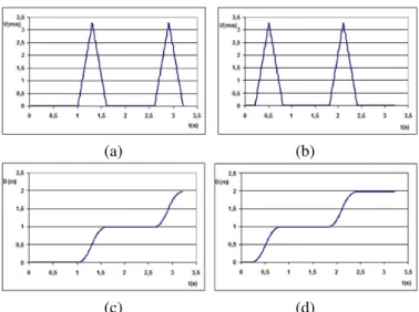
tds= (−0.0016 × step frequency + 0.2908) × tcycle Although tds could be calculated automatically if step
fre-quency is given, it is sometimes convenient to redefine tdsto have walking animations with various characteristics. By uti-lizing these equations, which define the kinematics of walk-ing, a velocity curve (time vs. velocity) is constructed for the left and right ankles. Figures 1 (a) and (b) illustrate the ve-locity of the left and right ankles versus time. The distance curves shown in Figure 1 (c) and (d) are automatically gener-ated using the velocity curves. Ease-in, ease-out effect, which is generated by speed up and slow down of the ankles, can be seen on distance curves.
(a) (b)
(c) (d)
Fig. 1. The velocity curves for (a) the left ankle and (b) the
right ankle. The distance curves for (c) the left ankle and (d) the right ankle.
5. MOTION OF THE SKELETON USING IKAN
Our work focuses on the analytical inverse kinematics meth-ods in which, the goal orientations are specified and the po-sition or rotation of joints are computed by using analytical methods. Moving a hand to grab an object or placing the foot to a desired position requires the usage of inverse kinemat-ics methods. We used a package, called IKAN, that provides a complete set of inverse kinematics algorithms for an an-thropomorphic arm or leg. It uses a combination of analytic and numerical methods to solve generalized inverse kinemat-ics problems including position, orientation, and aiming con-straints [2].
IKAN’s methodology is constructed on a 7 DOF fully revolute open kinematic chain with two spherical joints con-nected by a single revolute joint. In the arm model, the spher-ical joints with 3 DOFs are shoulder and wrist; the revolute joint with 1 DOF is elbow. In the leg model, the spherical joints with 3 DOFs are hip and ankle; the revolute joint with 1 DOF is knee.
Since leg and arm are both considered to be similar hu-man arm-like (HAL) chains, we only explain the details for the arm. The elbow is considered as parallel to the length of the body at rest condition. The z-axis is from elbow to wrist. The y-axis is perpendicular to z-axis and it is the axis of rotation for elbow. The x-axis is pointing away from the body along the frontal plane of the body. We assume a right-handed coordinate system. Similar coordinate systems are assumed at the shoulder and wrist. The projection axis is al-ways along the limb and the positive axis points away from the body perpendicular to the frontal plane of the body. The projection axis differs for left and right arm. Wrist-to-elbow and elbow-to-shoulder transformations are calculated to
ini-Fig. 2. Human walking behavior.
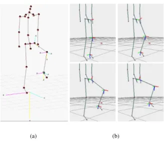
tialize the inverse kinematics solver. The arm is initialized with a Humanoid object and the shoulder, elbow and wrist joints. In the initialization part, the transformation matrices are computed and the inverse kinematics solver is initialized. The orientations of joints for the end-effector’s positioning of the left foot are seen in Figure 3 (a). The joint angles are found automatically according to the end-effector positions.
6. RESULTS AND CONCLUSIONS
Sample animations produced with our implementation can be found inhttp://www.cs.bilkent.edu.tr/∼gudukbay/
HumanModeling/SampleMotions.html. Figure 2 illustra-tes the human walking behavior. The position curves seen in Figure 2 are the trajectories of the left ankle, the right ankle and the pelvis. These position and velocity curves of each limb are generated automatically. The gait determinants com-pass gait, pelvic rotation, pelvic tilt, and lateral pelvic dis-placement are taken into account. The joint orientations for the end-effector positioning of the left foot can be seen in Fig-ure 3 (a). Goal-directed motion of the left leg can be seen in Figure 3 (b).
We tested our system on a Pentium-IV 1400 MHz (256 MB RAM) with 32MB Nvidia RIVA TNT2 graphics card and obtained an average performance of 397 frames/sec. The re-sults also show that the computational complexity of the sys-tem is independent of the complexity of the motion.
7. REFERENCES
[1] Humanoid Animation Working Group of Web3D Consortium, Specification of a Standard VRML Humanoid, Version 1.1, http://h-anim.org.
[2] Deepak, T., Goswami, A., Badler, N., “Real-time inverse kinematics techniques for anthropomorphic limbs”, Graphical Models, Vol. 62, No. 5, pp. 353-388, 2000.
(a) (b)
Fig. 3. (a) The joint orientations for the end-effector
position-ing of the left foot; (b) goal directed motion of the leg.
[3] Chadwick, J., Haumann, D. Parent, R., “Layered construc-tion for deformable animated characters”, Proc. of ACM SIG-GRAPH’89, pp. 243-252, 1989.
[4] Zhao, J., Badler, N., “Inverse kinematics positioning using nonlinear programming for highly articulated figures”, ACM Trans. on Graph., 13(4), pp. 313-336, 1994.
[5] Steketee, J., Badler, N., “Parametric keyframe interpolation in-corporating kinetic adjustment and phrasing control”, Proc. of ACM SIGGRAPH’85, pp. 255-262, 1985.
[6] Ko, H., Badler, N., “Animating human locomotion in real-time using inverse dynamics”, IEEE Comp. Graph. and App., 16(2):50-59, 1996.
[7] Badler, N., Phillips, C., B. and Webber, B., L., Simulating
Hu-mans: Computer Graphics, Animation, and Control, Oxford
Univ. Press, 1999.
[8] Bezault, L., Boulic, R., Magnenat-Thalmann, N., and Thal-mann, D., “An interactive tool for the design of human free-walking trajectories”, Proc. of Computer Animation, pp. 87-104, 1992.
[9] Bruderlin, A., Calvert, T., W., “Goal-directed dynamic ani-mation of human walking”, Proc. of ACM SIGGRAPH’89, pp. 233-242, 1989.
[10] Multon, F., France, L., Cani-Gasguel, P. and Debunne, G., “Computer animation of human walking: A survey”, J. of Vis. and Computer Animation, Vol. 10, pp. 39-54, 1999.
[11] Saunders, J.B., Inman, V.T. and Eberhart, H.D., “The major determinants in normal and pathological gait”, J. of Bone Joint Surgery, 35-A(3):543-558, 1953.