Closed-Form green's functions and their use in the method of moments

Jolectromagnetic Wave Interactions, pp. 1-37 ,·dited by A. Guran, R. Mittra and P. J. Moser

Series on Stability, Vibration and Control of Systems Series B: Vol. 12

@ World Scientific Publishing Company

CLOSED-FORM GREEN'S FUNCTIONS AND

THEIR USE IN THE METHOD OF MOMENTS

M. I. AKSUN

Electrical and Electronics Eng. Dept. Bilkent University

Ankara 06533, Turkey

and R. MITTRA

Electromagnetic Communication Laboratory Electrical and Computer Eng. Dept. University of Illinois at Urbana-Champaign

1406 W. Green Street Urbana, IL 61801

ABSTRACT

Derivation of the spatial-domain, closed-form Green's functions of the vector and scalar potentials are demonstrated for planar media, and their use in conjunction with the method of moments (MoM) is presented. As the first step of the derivation, the Green's functions are obtained analytically in the spectral domain for various sources viz., horizontal and vertical electric and magnetic dipoles embedded in a planar stratified media. The spatial-domain Green's function can be obtained from the Sommerfeld integral which is the Hankel transform of the corresponding Green's function in the spectral domain. The analytical evaluation of this transformation yields the closed-form, spatial-domain Green's functions which can be used in the solution of a mixed-potential integral equation (MPIE) via the MoM. This combi­ nation, i.e., the use of the closed-form Green's functions in conjunction with the MoM, results in a significant improvement in the fill-time of MoM matrices. In the conventional application of the spatial-domain MoM, the matrix elements are double integrals and they require the evaluation of the time-consuming Sommer­ feld integral for the spatial-domain Green's function. In the approach presented herein, the spatial-domain Green's functions are in closed forms, and the remaining double-integrals in the matrix elements are evaluated analytically. Thus, there are two factors in this approach that contribute to the improvement in the computa­ tion time: (i) elimination of the numerical integration to obtain the spatial-domain Green's functions; (ii) circumventing the need to carry out the numerical integration in the calculation of the MoM matrix elements.

1. Introduction

Electromagnetic modeling of printed structures in a stratified medium is an impor­

tant problem in computational electromagnetics, and has recently attracted widespread

attention. This is attributable to the increased use of multilayer microstrip geome­

tries in various applications of microstrip antennas

1

-6,

and in monolithic microwave

2

M. I. Aksun & R. Mittra

on the development of a rigorous and yet computationally efficient computer-aided

design tools for microstrip geometries in layered media. Hence, a variety of numeri­

cal techniques for accurate modeling and simulation of the electrical performances of

such circuits have been proposed and studied extensively. These include the method

of moments (MoM)

9

and its variants; the finite element method (FEM)

_10;

the finite

difference time domain (FDTD) method

11

_{, and quasi-static methods based on con­}

formal mapping

12_.

_{Among these approaches, the spatial and spectral domain MoM}

approaches are the most commonly used numerical techniques for the rigorous anal­

ysis of printed geometries in multilayer planar media.

The use of the MoM in the analysis of microstrip geometries requires the compu­

tation of the Green's functions for layered media, which are represented analytically

in the spectral domain and transformed into the spatial domain from the spectral­

domain representations via the Hankel transform. The resulting spatial-domain repre­

sentation, also referred to as the Sommerfeld integral

13,

is a one-dimensional integral

over an infinite range with the Hankel function as its kernel; hence, its numerical eval­

uation is computationally inefficient unless an acceleration technique is used. Since

the Green's functions in the spectral domain are expressible in closed forms, the use

of the spectral-domain MoM in the analysis of microstrip geometries had attracted

much interest

14_-17•

Although, relatively speaking, the spectral-domain MoM is more

efficient in terms of computation time than some of the other numerically rigorous

techniques, it is still quite time-consuming to implement. This is because, in this

approach, the MoM matrix elements are double integrals of complex, slowly-decaying

functions over infinite ranges. To overcome the difficulty introduced by the slowly­

decaying nature of the integrand, the spectral-domain approach is usually employed

in conjunction with an acceleration technique in which the asymptotic part of the

integrand is subtracted from the original integrand and its contribution is calculated

either analytically or in a numerically efficient manner

18_• 19_.

However, even with the

use of this tactic, this computation remains expensive, because the integrands are os­

cillatory functions of the spectral domain variables, and for the self-terms, for which

the observation region coincides with the source region, the convergence is still quite

slow. The computational inefficiency plagues the spatial domain MoM as well, since it

involves the evaluation of at least a three-dimensional integral for the matrix element,

one of which is the Sommerfeld integral. However, since the remaining double-integral

is over a finite domain, the spatial-domain MoM can be made computationally inex­

pensive if the Sommerfeld integrals can be evaluated efficiently.

A number of different techniques have been proposed for the efficient evaluation of

the Sommerfeld-type integrals by employing acceleration techniques. These include

the Shank's transformation, the Euler transformation and the method of averages.

Among these, the method of averages has been demonstrated to be the most efficient

for the evaluation of the Sommerfeld-type integrals

20_•

_{These techniques require the}

numerical evaluation of the integral at several intervals that leads to a series, whose

convergence is accelerated via a nonlinear transformation. In this approach, it is

necessary to perform a numerical integration over a portion of the infinite range of

the original integral. Thus the efficiency of this technique is determined by the extent

1. Closed-Form Green's Functions . . . 3

of the interval over which one needs to perform the numerical integration to predict

the end result sufficiently accurately. In addition, since the Sommerfeld integral is

a parametric integral, with the radial distance p as the parameter, the process of

acceleration described above has to be performed for each value of the parameter,

which is usually on the order of hundreds for typical applications of the spatial­

domain MoM. Consequently, even if the method of averages enabled us to compute

the Sommerfeld integral efficiently for one value of p, it would be quite expensive to

employ this technique directly in conjunction with the spatial-domain MoM which

calls the evaluation of the above integral for many p. One approach to circumventing

this difficulty is to precompute the values of the Green's functions for a range of radial

distances and curve-fit these values locally using low-order polynomials

21_.

_{Even so,}

the integral must be evaluated for tens of radial distances for the purpose of curve­

fitting, because of the sharp changes in some Green's functions caused by phase

cancelations.

Recently, yet another approach has been proposed which appears to resolve all of

these difficulties mentioned above. This approach was first proposed

22

_{for a thick,}

single layer microstrip geometry, and later extended to multilayer planar geometries

with arbitrary thicknesses

23_• 24_•

_{It takes advantage of the fact that the Sommerfeld in­}

tegral can be integrated analytically if the integrand, apart from the kernel HJ

2

_l(k

pp

),

can be approximated by complex exponentials. With this approach, the numerical

integration, which causes computational inefficiency in the acceleration techniques

mentioned above, is completely eliminated. Instead, the burden of the numerical

algorithm falls on the task of approximating the spectral-domain Green's functions

in terms of complex exponentials. Naturally, one might raise the questions regard­

ing the computational efficiency and robustness of this technique and the difficulties

arising in the process of applying the algorithms for the exponential approximation.

Before addressing these questions, it would be useful to describe some of the recent

improvements

25

_{introduced in the technique. In its original form}

22

_{Prony's method}

was used for the exponential approximation

2_6,

_{which required the same number of}

samples as the number of unknowns, i.e., twice the number of complex exponentials

( one for the coefficient and one for the exponent). One consequence of this was that

it was difficult to account for the rapid variations of the integrand in the spectral

domain without using a large number of complex exponentials, and this phenomenon

is attributable, in part, to the uniform sampling required in Prony's method. Al­

though the least-square Prony's method improves its ability to account for the rapid

changes with a moderate number of exponentials

23_,

_{it still requires several trial and}

error iterations, because of the noise sensitivity of the Prony methods

27,

_{which render}

the technique to be inefficient and not robust. As a solution, another exponential ap­

proximation technique, called the generalized pencil of function (GPOF) method

2_8,

is employed in casting the Green's functions into closed forms

24_•

_{The GPOF method}

has turned out to be quite robust and less noise sensitive when compared to the orig­

inal and least-square Prony methods, and also provides a good measure for choosing

the number of exponentials used in the approximation. However, it still requires one

to study in advance the spectral-domain behavior of the Green's function in order

4 M. I. Aksun & R. Mittra

to decide on the approximation parameters like the number of sampling points and the maximum value' of the sampling range. In addition, since the approximation techniques, such as the Prony and the GPOF methods, require the function to be sampled uniformly, one would need to take thousands of samples in order to be able to approximate a slow converging function with rapid changes (even if this were to occur in a small region), which is a typical behavior of the spectral-domain Green's functions of the scalar potentials in a thin substrate. Because of these difficulties, the technique of deriving the closed-form Green's functions and subsequently using them in MoM applications is not considered to be robust, and thus could not be used conve­ niently for the development of a general-purpose electromagnetic software. Recently, a new approach based on a two-level approximation has been proposed to overcome these difficulties, and it has been demonstrated that the new approach is very robust and computationally much more efficient than the original one or its variants. The two-level approach divides the range of approximation into two parts, the first of which covers the region where the function to be approximated has rapid transitions, whereas the function is smooth in the second region. Thus, it is no longer necessary to take thousands of samples to account for a rapid transition that occurs in a small part of the entire range, and this results in a significant reduction of the number of data points to be processed in deriving the exponential approximation, which, in turn, translates into a substantial saving in the computation time. Throughout this chapter., this new approach is referred to as the two-level approach while the original technique is called the one-level approach.

With the introduction of the robust and efficient approach in the derivation of the closed-form Green's functions, the use of the MoM in the spatial domain becomes very attractive for the analysis of printed geometries in a multilayer environment. The Sommerfeld integral is now completely eliminated and the calculation of the matrix elements in the spatial-domain MoM now only requires double integrals over finite ranges that are evaluated numerically. It has been demonstrated that even the elimination of only the Sommerfeld integrals improves the computational efficiency of the spatial-domain MoM significantly29_{• It has also been recently demonstrated}30

that, with the analytical approximation of the remaining double-integrals, the com­ putational efficiency of the evaluation of the matrix elements is further improved. Consequently, a substantial improvement in the matrix-fill time is achieved by ana­ lytically evaluating all of the integrals involved in the spatial-domain MoM.

Section 2 describes the derivation of the closed-form Green's functions and includes the derivation of the spectral-domain Green's functions, discussions on the difficulties associated with the original one-level approach, and assessment of the robustness and computational efficiency of the two-level approach. Section 3 describes the use of the closed-form Green's functions in conjunction with the MoM and provides the analytical evaluation of the MoM matrix elements together with the necessary integral identities.

2. Closed-Form Green's Functions

1. Closed-Form Green's Functions . . . 5

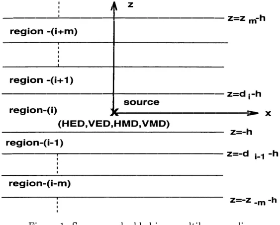
Let us consider, for the sake of illustration, a planar, multilayercd medium shown in Fig. 1 where it is assumed that the layers extend to infinity in the transverse directions. The source, (RED, HMD, VED or VMD) is embedded in region i and the observation point can be located in an arbitrary layer. Each layer can have different electric and magnetic properties (€,,µ,) and thickness (d;). The perfect electric or magnetic conducting planes and half-space are also regarded as layers in this formulation. The procedure for deriving closed-form expressions for the Green's

j�

z

---�---11---

Z=Z m-h region -(i+m) region -(i+1)

---11---

Z=d j-h source region-(i)

.,,'---=�

(HED, VED,HMD, VMD) Z=-h region-(i-1) X ---.--- z=-d 1_1 -h region-(i-m) Z=-Z .m ·h

Figure 1: Sources embedded in a multilayer medium. functions entails the following steps:

1. Derivation of the Green's functions in the spectral domain. (a) Green's functions are derived in the source layer.

(b) Green's functions in the observation layer are obtained by using an iterative algorithm applied to each TE and TM component of the Green's functions in the source layer.

6

M. I. Aksun & R. Mittra

(a) Spectral-domain Green's functions are approximated in terms of complex exponentials obtained from the GPOF method after the direct terms have been extracted.

(b) Closed-form Green's functions are obtained analytically by using the Som­ merfeld identity for each of the complex exponentials.

All of the Green's functions, presented herein, are for the vector and scalar poten­ tials that are indeed not defined uniquely in stratified media3_1• 3_{2. Therefore, different}

sets of Green's functions for the vector and scalar potentials can be chosen to satisfy the same boundary conditions. The following notation for the Green's function is commonly used and referred to as the traditional form33_:

(1)

for the vector potentials, and G�:r and G�•,m _{for the scalar potentials. Note that,} in this representation, the scalar potentials of the point charges associated with the horizontal and vertical dipoles are not identical. This leads to some difficulties in the solution of the mixed potential integral equation for a geometry where both the horizontal and vertical sources (HED and VED or HMD and VMD) are present at the same point, as in the case of a microstrip etch fed by a vertical probe. To overcome this difficulty, an alternative form has been suggested32 _{for the Green's functions and}

these representations are given in Appendix A.

2.1. Green's Functions in the Spectral Domain

The spectral-domain Green's functions of the vector and scalar potentials can be obtained from the electric and magnetic fields generated by a current dipole J

=

I

0l8(r)a., where a is a unit vector. For the sake of illustration, the field components for an HED in a multiiayer media, Fig. 1, can be written in the source layer (layer i) as follows34_:

(2)

(3)

where the z dependence of the fields in the source region is written as the sum of the direct term and up- and down-going waves due to the reflections from the boundaries at z

=

-h and z

=

d; - h, respectively, and

+

and - signs are for z > 0 and z

<

0,

respectively. The coefficients of the up- and down-going waves can be obtained in terms of the generalized reflection coefficients by applying the appropriate boundary conditions: (i) the down-going waves for z > 0 are the consequence of the reflections of the up-going waves at z

=

d; -

h;

and (ii) the up-going waves for z < 0 are the

1. Closed-Form Green's Functions . . . 1

consequence of the reflections of the down-going waves at

z

=

-h.

It should be noted that the other field components can be easily derived from the z-components of the fi.elds34_{, so they are not included here. After having obtained the field components,} the components of the vector potentials and the scalar potential can be derived from the following relations:

'v X

A=

µ;H

₍₄₎

,P_{d =} _ 'v x A ₌ I0l 8,p

(5)

jwµ;E; jw 81'

where ,Pd and ,p are the scalar potentials for the dipole element and a point charge, respectively, and l' is replaced by x' or

y'

for an HED ( depending upon the orientation of the dipole) and replaced by z' for a VED. Given below are the expressions of the spectral-domain Green's functions (traditional form) in the source layer for HED, HMD, VED and VMD sources. They read:

HED: HMD: G-_{,.,, = 2 .}A

-µ;

[k.,,k,; (A" + B") jk,;z k . k2 h h

e

J z,

_p

+

k�!'• (Di:

-

C;:)e-jk,,z] p -f.; [k.,,k,, (Am+ Bm) jk,,z = _{? 'k k2 h h}

_e

-J z;

_P

+

k�!·· (Di:'

-

Cf')e-i"•,'] p

(6)

(7)

(8)

(9)

(10)

(11)

8

M. I. Aksun & R. Mittra

VED:

VMD:

{jA = _!!}_[e-ik,; lzl + A"_ZZ e-ik,,z + B"eik,, •]

j2kz, V V

{jq• = __ l_[e-jk,; lzl + c•z e-ik,,z + n•eik,,•1

j2kz, fj V V

(12)

(13)

(14)

(15)

where Gj·F _{denotes the spectral-domain Green's functions for the vector potentials in} the direction-i due to a unit j-directed current element; GJ•,m represents the Green's function of the scalar potential in the spectral domain due to a unit i-directed electric or magnetic current element; k; = k: + k:, ; the superscripts A and F represent the magnetic and the electric vector potentials, respectively; and, q. and qm represent the electric and magnetic scalar potentials, respectively. The coefficients, At': , B::': , c•,m _n•,m _{are functions of the generalized reflection coefficients R}

rE,TM, and are h,v , h , u given by A"•_h m

+

Be,m h

=

c:·m

=

+

D�·m

+

A"·m V

+

e-ik,. (d,-h) kj.i+I [I _E,TM e-ik,.(d,-h) I

k;i-1 -jk,, (d,+hl]MTE,TM E,TMe ' i -jk,. (d;-h) kj.i+I [ -jk,.(d;-h) e _{• M,}TE e • k;i-1 -jk, (d,+hl]M™·TE M,TEe ' i -jk,. hkj.i-1 [ -jk,.h e _• E,TM e • kj.i+I _E,_TM e-ik,, (2d,-hl]M!, E,TM -jk,. h Je;i-1 [ -jk,.h e _{• M,TE -e •} kj.i+I -jk,. (2d,-hl] M™·TE M,TEe ' i -jk, h fe,i-1 [ -jk,.h e _{' 1'M,TE e} Je;i+l -jk,. (2d;-h)l MTM.TE M,TEe ' 1 i

(16)

(17)

(18)

( 19)

{20)

where

1. Closed-Form Green's Functions . . . 9 B!•m

=

_{e-ik,, (d,-h) �:�/TE[e-ik,, (d,-h)}

+ �tlTEe-ik,, (d,+h)]MfM,TE

c:,

m

=

e-ik,, h ��\.Bf-e-ik,,h

+

_{'VJ'M,TE Ri,i+I e-ik,. (2d,-hl]MTM,TE ' i}

D!•m _{e-ik,, (d,-h) �i�TE[-e-ik,,(d,-h)}

+

_{' VJ'M,TE Ri,i-1 e-ik,. (d,+hl]MTM,TE ' i}

•1,,TE,TM -

[1

Ri,i+l Ri,i-1 _{-jk,. 2d,1-1} m ; - - ·vrE,TM'VJ'E,TMe '

pi+I,j + j"Jj,j-1 e-ik,,2dj Ri+l,i •vrE,TM •vrE,TM

'VJ'E,TM

=

₁

_{R Ri,i-1 -ik, - 2dj} - i,i+PvrE,TMe 1 (21) (22) (23)

(24)

(25)

Here R and R are the Fresnel and generalized reflection coefficients34 _{for which the}

subscripts

TE

and

TM

represent the polarization of the wave, and the superscripts ( i, i - 1 ) or ( i, i

+

1 ) show the layer numbers. The subscripts

h

and

v

used in the

coefficients (16-23) represent the orientation of the source, horizontal and vertical, respectively, while the superscripts e and m denote the type of the source, electric and magnetic, respectively. It should be noted that the horizontal Green's functions

- A <' - A F (';A,F (';A,F

for the y-oriented dipoles can be obtained simply by setting GYY. = G"';, , �= �, and ai•,m_=G�•,m_.

The amplitudes of the up- and down-going waves in a layer different from the source layer are �elated to those in the adjacent layers by,

(26) where Ai and A.i+I are the amplitudes of the down-going waves in layers

j

and

j

+ 1, respectively, (j

=

i - m), T is the transmission coefficient, and Z-m is the distance between the lower boundary of the source layer i and the lower boundary of layer

j,

Fig. 1. Similarly the amplitudes of the up-going waves in layer

j

=

i + m can be written as

T· -e-i(k,,_, -k,; H•m-1 +d, -hl

At = At _{1 i-i} i - t ,J _ . (27)

1 - R · · 1R · · _{J,J - J,J+} 1 e-i.1:,,u,

Therefore, starting from the source layer, the field expressions for any layer can be obtained iteratively.

10

M. I. Aksun & R. Mittra

2.2. Closed-Form Green's Functions in the Spatial Domain

Since the principal goal of this section is to introduce a robust and efficient tech­ nique to obtain the spatial-domain Green's functions in closed-forms for planar layered media, it would be useful to first provide the definition of the spatial-domain Green's functions

aA,F,q. ,qm

=

2_ f dk k H(2> (k p)GA,F,q.,qm (k )

4?r

ls1P

P P O P P (28)

where,

G

and G are the Green's functions in the spatial and spectral domains, re­ spectively,

HJ

2

>

is the Hankel function of the second kind and

SIP is the Sommerfeld

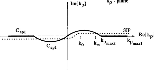
integration path defined in Fig. 2. The Sommerfeld integral given in (28) cannot be

kp - plane

. . . �A'

_{Re[ kp]}

kPmaxl

Figure 2: Definition of the Sommerfeld integration path, and the paths Capl and Cap2

used in one- and two-level approximations.

integrated analytically, except for a few special cases. However, if G, the spectral do­ main representation of the Green's function in the integrand can be approximated in terms of complex exponentials, the analytical evaluation of the integral (28) becomes possible via the Sommerfeld identity

(29)

Therefore, the crucial step in the derivation of the closed-form Green's functions is the exponential approximation of G. Since the approximation techniques used for this problem, namely the original Prony, the least square Prony and the GPO F methods, require uniform samples along a real variable of a complex-valued function, one might think of choosing the integration path in (28) along the real k_P axis so that G can be sampled along a real variable. However, one should note that k;

=

k2 _{- k; and} sampling along the real kP axis results in an approximation in terms of exponentials of k_P which cannot be cast into a form of exponentials of k, as required in the application

1 . Closed-Form Green's Functions . . . 1 1 of the Sommerfeld identity (29). Hence, the SIP must be deformed such that the mapping is from a real variable, viz., the running parameter of the mapping, onto the complex kz plane. In the original approach, a deformed path on kP plane, denoted by Cap2 in Fig. 2, was used to sample the function to be approximated, while in the new approach, called the two-level approach, a path formed by the paths Cap2 and Capl is employed. The details of these approaches together with the advantages and disadvantages will be discussed in the following sections.

For a general-purpose algorithm, the spectral-domain Green's functions are ob­ tained for a multilayer medium and neither surface wave poles nor the real images are extracted. The extraction of the surface-wave poles (SWP) and the real images helps the exponential approximation techniques by rendering the Green's functions in the spectral domain well-behaved and rapidly converging functions. However, since the contribution of the SWPs is small for geometries on a thin substrate, and it is not possible to find the real images for multilayer planar structures analytically except for some simple cases such as single and double layers, it is likely that the ad­ vantage gained by manipulating the Green's functions in a manner described above would be limited to a restricted class of planar geometries and would not lead to a general-purpose or robust algorithm.

Note that to be able to use Sommerfeld identity, the approximation of the spectral domain Green's functions, Eqs.

_(6)-(15),

must be performed for the terms with the square brackets, i.e., the terms other than those that are k� . In addition, k,, and ky parameters in G1,/ and G1/, respectively, are excluded i� the approximation and their contributions are added in the spatial domain ( after having obtained the spatial domain representations of

0

Z;F and 0f( ) by differentiating them analytically with respect to x and

y,

respectively.

2.2. 1 . Original One-Level Approximation

The deformed path Cap2 on the kp plane is defined as a mapping of a real variable

t

onto the complex kz plane by kz;

=

k; [-jt

+

(1 - T.t )], _o2

0

$ t $ To2

(30) The Green's functions are sampled uniformly on

t

E [O, To2], which maps onto the path C_{ap2 with k}Pm•••

=

k; [l +T;2]

1_{!2 in the k}

p-plane, and then approximated in terms of exponentials of

t

which can be easily transformed into exponentials of kz; . This scheme is called the one-level approximation app1oach because the complex function to be approximated is sampled between O and

T

02 , and is assumed to be negligible

beyond

T

02•

It is instructive to consider the practical details of the implementation of the expo­ nential approximation along the path defined in Eq. (30). It is of utmost importance for the success of this approach to choose, judiciously, the approximation parameters, viz., the interval

T

02 , the number of exponentials to be used in the approximation,

1 2

M. I. Aksun & R. Mittra

and the number of samples in t E [O, T

o2

] . To illustrate the implementation of the

one-level exponential approximation and the difficulties involved, the spectral-domain

Green's function for the scalar potential due to an x-directed dipole, G! , is given in

Fig. 3, for a geometry of four layers at 30 GHz: 1st layer- PEC; 2nd layer- e,

2

=12.5,

d

2

=0.03 cm; 3rd layer- e,

3

=2.1 , d

3

=0.07 cm; 4th layer- free-space, and the source and

observation planes are chosen at the interface of the second and third layers. It is

G!·

4.0 \ -- Real ···-·-···- hnag:inary

\

2.0 .. ··· _{···-··· ···} 0.0 -2.0 -4.00.0 0.1 0.2 0.3 0.4 0.5 0.6 0.7 0.8 O.!> 1.0

Figure 3: The magnitude of the spectral-domain Green's function G!• along the path

Cap2 ·

1st layer- PEC; 2nd layer- 1:,

2

=12.5, d

2

=0.03 cm; 3rd layer- e,

3

=2. 1 , d

3

=0.07

cm; 4th layer- free-space, freq=30 GHz.

evident from Fig. 3 that Green's functions can have sharp peaks and fast changes for

small

t,

which maps to the far-field region in the spatial domain. Hence one needs

to sample the Green's function given in Fig. 3 at a period of less than 0.05 along t

so that the fine features of the function can be captured in the approximation. The

choice of T

o2

is another parameter that competes with the period of samples, be­

cause a large T

o2

corresponds to large number of samples and translates into a longer

CPU time. Fortunately, for the example given in Fig. 3, the Green's function decays

quite rapidly in the spectral domain. Hence it is sufficient to sample the Green's

function only as far as T

o

2

=

5, which requires 200 samples if 6.t is chosen to equal

0.025. The spatial-domain Green's function is obtained via the GPOF method us­

ing the above approximation parameters (T

o2

=5, number of samples=201, number of

exponentials=13) and compared to the result obtained from the numerical integra­

tion, which are labeled as Apprx. and Exact, respectively, in Fig. 4. Although, as it

1. Closed-Form Green's Functions . . . 13 15.0 ,----�--�----�---�---, 14.0 13.0

---12.0

- - -

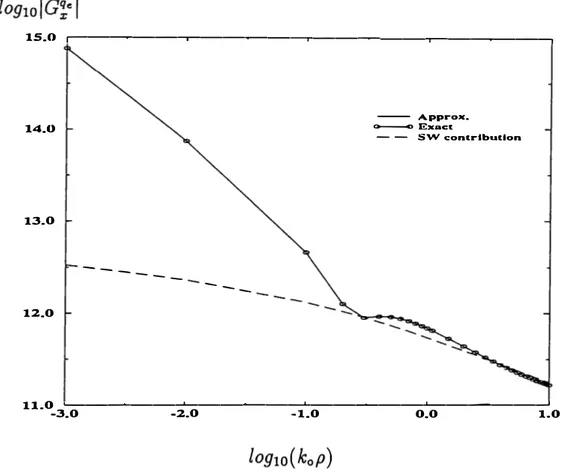
---- A ppro•. a----o E,i:aet. - - SW cont.ribur.lon 11.0 �----�----�---�----� _{-3.0 -2.0 -1.0 0.0 1.0}

Figure .4: The ma.gnitude of the Green's function for the sca.la.r potentia.l a.nd the surface wa.ve contribution. 1st la.yer- PEC; 2nd la.yer- €,2=12.5, d2=0.03 cm; 3rd la.yer- €,3=2. l, d3=0.07 cm; 4th la.yer- free-spa.ce, freq=30 GHz.

wa.s mentioned a.hove, the SWPs a.re not extra.cted from the spectra.1-doma.in Green's function prior to the exponentia.l a.pproxima.tion, the contribution of the SWPs is a.lso shown for the purpose of compa.rison. One ca.n dra.w the conclusion tha.t the exponen­ tia.l a.pproxima.tion a.lgorithm (GPOF) works well within the influence ra.nge of the SWPs. Beyond tha.t a.n a.symptotic a.pproxima.tion together with the surfa.ce-wa.ve contribution ca.n be used to a.pproxima.te the spa.tia.1-doma.in Green's functions35_• 3_{6 •}

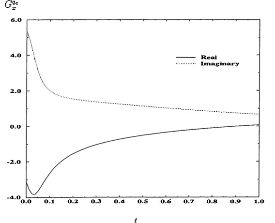
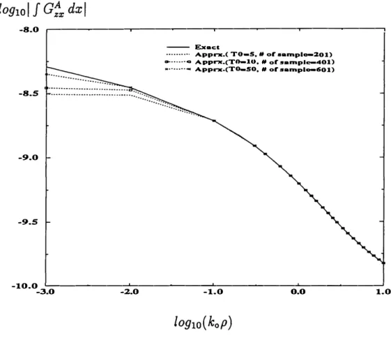
Unfortuna.tely, not a.11 the Green's functions ha.ve ra.pidly deca.ying spectra.1-doma.in beha.vior, of the type in the exa.mple given a.hove in Fig. 3. For exa.mple, the spectra.1-doma.in Green's function for the vertica.l component of the vector potentia.l due to a. HED, G1,Jikx = a:_y/jk_y (7), does not deca.y a.s fa.st a.nd, moreover, ha.s a. rela.­ tively sha.rp pea.k which requires sa.mpling a.lmost a.s frequently a.s tha.t of the exa.mple given in Fig. 3 (see Fig. 5). To demonstra.te the effect of the choice of a.pproxima.tion pa.ra.meters, the Green's function J G1x

dx

( = F-1 { G1xfi kx}) is given for the sa.me a.pproxima.tion pa.ra.meters a.s those of the a.hove exa.mple (Ta2=5, number of sa.m­ ples=201) a.nd compa.red to the results obta.ined by the numerica.l integra.tion of the spectra.l-doma.in representa.tion of the Green's function a.nd to the results obta.ined by using different a.pproxima.tion pa.ra.meters in Fig. 6. We observe tha.t the a.pprox­ ima.ted Green's functions do not a.gree well with the exa.ct solution for sma.11 va.lues of

p.

This is beca.use the spectra.1-doma.in Green's function is not sa.mpled fa.r enough

14 M. /. Aksun & R. Mittra 0.1 0.1 0.0 ··· -0.1 I - Roal ···· ··· lmaa;lnary -0.1 '---�----�---..__ ____ ...J _{0.0 s.o 10.0 15.0 20.0}

Figure 5: The magnitude of the spectral-domain Green's function Gf,,/j k_,, along the path Cap2 · 1st layer- PEC; 2nd layer- E,2=12.5, d2=0.03 cm; 3rd layer- E,3=2. 1, d3=0.07 cm; 4th layer- free-space, freq=30 GHz.

to get an accurate near-field distribution. However, if the value of T02 is increased, the agreement between the approximated and exact Green's functions is improved at the expense of the computation time provided that the frequency of sampling is kept constant.

From the above discussion, it can be concluded that the one-level approximation approach cannot be made fully robust and suitable for the development of CAD soft­ ware. As was mentioned above, this is because it requires the users to first investigate the spectral-domain behavior of the Green's function and then perform a few iter­ ations to find the best possible combination of the approximation parameters. To circumvent these difficulties, a two-level approximation scheme has been developed in conjunction with the use of the GPOF method and its details are given in the following section.

2.2.2 Two-Level Approach

To alleviate the necessity of investigating the spectral-domain Green's functions in advance and the difficulties caused by the trade-off between the sampling range T02 and the sampling period, the approximation is performed in two levels. The first part of the approximation is carried out along the path _Capl, and the second along the path _Cap2, as shown in Fig. 2. Note that the second part of the approximation

1 . Closed-Form Green's Functions . . . 1 5 -8.0 .---�----�---�---, -8.S -9.0 -9.S - Ex•ct ··· ···· ··· Apprx.( TO-S. # or ••mpl-201) -· ···ci A pprx.(T0-10, # ol' sample-401) ... Apprx.(T0-50. # or ••mpl-601)

-10.0 '---�----�---�----� _{-3.0 -2.0 -1.0 o.o 1.0}

Figure 6: The magnitude of the Green's function for the vector potential

J

G1

,,

dx.

1st layer- PEC; 2nd layer- f,2= 12.5, d2=0.03 cm; 3rd layer- f,3=2. 1 , d3=0.07 cm; 4th

layer- free-space, freq=30 GHz.

is the same as the one-level approximation scheme described in the previous section, except th_at now the value of To2 (kPmas• = k[l

+

T;₂]112) can be set in advance such

that kPmas• � km where km is the maximum value of the wavenumber involved in the

geometry.

To illustrate the procedure of the two-level approximation, we will first outline the necessary steps and then provide some of the details. The steps are:

• Choose To2 such that k_Pmas• � km: For example, since GaAs is the highest

dielectric constant layer (fr(GaAs) = 12.5), then km = ./mko, and To2 can

be safely chosen to be 5.

• Choose Toi , i.e., kPmasi = k[l

+

(Toi

+

To2 )2]112, and the number of samples

in the range [k_Pmas2 ' kPmasi l · The choice of Toi is not very critical as long as

one chooses kPmas, large enough to pick up the behavior of the spectral-domain

Green's function for large kp. Also, since the spectral-domain behaviors of the

Green's functions are alw:i.ys smooth beyond k_{Pmas2 ' it is not necessary to have} a large number of sampies on (kPmu2 l kPmas, J . Typical values could be 200 for

Toi and 200 for the number of samples.

16 M. /. Aksun & R. Mittm

method: Sampling along the path

Cap!

can be performed by varying t between

0 and T

01

uniformly in k

z

=

-jk[T

02

+

t] .

• Subtract the function approximated for the range of k

P

E [ k

P

mo%

2 ,

k

P

ma%, ] from

the original function: The remaining function will be non-zero over a small range

of k

p

( E [O, k

Pma%2

]) so that one can pick up the fine features of this function

without employing a relatively large number of sampling points.

• Sample the remaining function along the path

Cap2

uniformly and approximate

it by using the GPOF method: Sampling along the path

Cap2

can be performed

by varying t between O and T

o2

uniformly in k

z

= k[-jt

+

(l - t/T

02

)].

The parameters that must be fixed by the user in advance are the limits of the

sampling ranges T

o

i and To

2

for the first and the second parts of the approximation,

respectively, and the number of samples along the paths

Cap!

and

Cap2 ,

which respec­

tively correspond to the first and second parts of the approximation. Although it

appears the number of parameters that are to be decided by the user is greater than

for the one-level approximation, these parameters need be determined only once for

the class of geometries that are of interest. Also, they are used for the approximation

of any component of the dyadic Green's function and for any geometrical constants.

Finally, the choice of these parameters do not require an investigation of the function

to be approximated in advance because they can be chosen for the possible limits of

the geometrical constants.

To demonstrate the robustness of the technique, the choice of the parameters and

the application of the above procedure, the Green's function

J

c:

x

dx

is obtained for

the same geometry as considered in Section 2.2.1. Let us first write the parametric

equations describing the paths

Cap!

and

Cap2

for the first and second parts of the

approximation, respectively

For

Cap!

For

Cap2

-jk;[T

o2

+

t]

0 :S t :S T

o

i

k;[-jt + (l - -

_T

t )] O :S t :S T

02 o2

(31)

(32)

where t is the running variable sampled uniformly on the corresponding range. Then,

the above procedure is followed step by step as:

• T

o2

=

5 is chosen, for which k

Pm

o%2

=

k; [l

+

T;

2

J

1

!

2

> km

=

Vl2.5

ko

• T

01

= 400 is chosen to ensure that the behavior of G1

x

/ik

x

for large k

p

is

captured. This choice for T

o1

is not critical; for instance, a value of 300 or 500

could have been chosen instead. Since there is no fine feature to be modeled

in this range, i.e., since the function is smooth, one can keep the range large

without having to use a large number of samples. Therefore, the number of

samples is chosen to be 50.

1 . Closed-Form Green's Functions . . . 17

•

G1,Jjk., is sampled along the path Capt and the GPOF method is applied.

fJin Otn

=

--;---k j J i N,

L

bine/3,nt n=l N,

=

I:

a1ne-0'1nk_zi n=l (33) (34) where b1n and fJ1n are the coefficients and exponents obtained from the GPOF method, and N1 is the number of exponentials used in this approximation. The choice of the number of exponentials is based upon the number of significant singular values obtained in an intermediate step of the application of the GPOF method. For this specific problem, five exponentials are chosen to approximate the Green's function over the range of kp E [kPmoz2 > kPmoz, l · It is necessary to transform the coefficients b1n and the exponents fl1n is necessary to cast the ap­ proximating function into a form suitable for the application of the Sommerfeld identity (29). This, in turn, implies that the approximating function must be an exponential representation in terms of kz; . Hence, a1n and a1n are obtained in terms of b1n and f11n in (34).

• The approximating function J(kp) is subtracted from the original function G1_.,/jk.,, which guarantees the remaining function to be negligible beyond

kpmax2 ·

(35) Note that the first integral is evaluated along the path Cap2 because the inte­ grand is negligible on CapI , but the second integral is evaluated along _{Cap2+ Capl ·} Therefore, the Sommerfeld identity (29) can be applied to the integrals in (35). The remaining function is sampled along the path Cap2 with 100 samples. Since the maximum range for the sampling (kPm ... 2 ) is rather small compared to that of the one-level approximation scheme, the frequency of sampling can be made quite high without substantially increasing the number of samples. For all practical purposes (including the worst case situation) the choice of 200 as the number of samples is more than sufficient to get a good approximation.

QA

�

�

·i." -

J(kp) �

I:

o.ne/J•nt

=

I:

a2ne-"•nk,; J x _{n=I n=l} f12nT02 a2n

=

k; ( l + jTo2) ;

(36)

(37)

18 M. I. Aksun & R. Mittra

where b2n and /32n are the coefficients and exponents of the exponentials of

t

obtained from the application of the GPOF method, and a2_n and a2n are the

coefficients and exponents of the exponentials of k,, . The number of exponen­ tials

N

2· in this part of the approximation is chosen to be 8, again by the number of significant singular values.

• By following the previous steps, the spectral-domain Green's function can be written as

(38) Also the spatial-domain Green's function can be cast into a closed-form by substituting this approximation of the spectral-domain Green's function into Eq. (28) , and then employing the Sommerfeld identity Eq. (29) for each term to yield

(39) where Tin =

jx

2

+

y2 - a?n and T2n =

jx

2

+

y

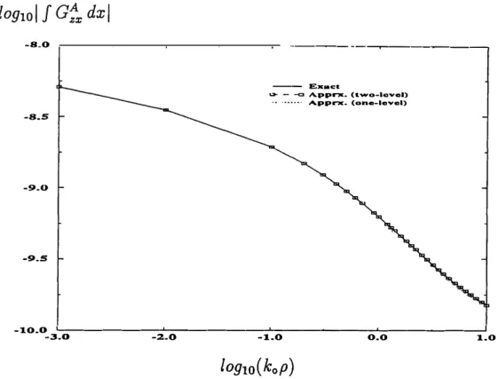
2 - a�n are the complex dis­ tances.

In summary, the approximation parameters chosen here for the first part of the approximation are: Toi = 400; To2 = 5; number of samples=50; and, number of expo­ nentials=5. Likewise, for the second part of the approximation these parameters are: number of samples= lOO; and, number of exponentials=8. Note that the total number of exponentials used in this approximation is 13. The Green's function derived by employing the above procedure is plotted in Fig. 7, along with the data obtained from direct numerical evaluation of the Sommerfeld-type integral (exact) . Also plotted in Fig. 7 are the results derived from the one-level approximation approach with the following parameters of approximation:

T

0 = 200; number of samples=400; and the number of exponentials=l3. Note that the values of the parameters used in the one­ level approximation are chosen to reduce the computation time without sacrificing too much accuracy. However, those of the two-level approximation are typical values and the number of samples for the second part of the approximation can even be reduced to 50 with little or no change in the results. The CPU times on the SPARCstation 10/41 for two approximation techniques for the above example are compared when the same number ( =13) of total exponentials are used for different approximation parameters. The results are presented in the tabular format below:

Approximation Approximation Parameters CPU time (sec)

one-level

T

0 = 200,

N,

= 400 198.0

one-level To = 200, Ns = 500 382.0

two-level Toi = 400, N,1 = 50 To2 = 5, N,2 = 50 1 .2

-s.o

-9.5

1. Closed-Form Green's Functions . . . 19

---�--- Exact

1> - -c:i Apprx. (two-lavel) · · · · · A.pp,nr. (on-level)

-io.�3-'--:.0::---:_2�-o=---1="".--=-o---o� . ..,.o---'1.o

Figure 7: The magnitude of the Green's function for the vector potential J

Gf

.,

dx.

1st layer- PEC; 2nd layer- f,2

=

12.5, d2

=

0.03 cm; 3rd layer- e,

_{3 =}

2.1 , d

_{3 =}

0.07 cm; 4th

layer- free-space, freq

=

30 GHz.

where N, is the number of samples in the one-level approximation scheme while N

s1

and N,2 are the number of samples of the first and second parts of the approximation,

respectively, in the two-level approximation approach. It is obvious that the two-level

approximation approach improves the computational efficiency significantly.

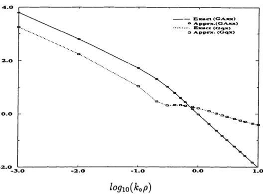
The robustness of the two-level approach can be demonstrated by casting the

other Green's functions into closed forms with the use of the same approximation

parameters as those employed for J

Gf

.,

dx,

viz.,

T

o1

= 400,

N,,

= 50 T

o

2

=

5,

N,

2 =

100. The normalized Green's functions of the vector and. scalar potentials due

to HED and VED sources are obtained (41rG:

.,

f µ

3

, 41re

3

G�, 41rGf

z

/ µ3 and 4H

3

Gn

following the two-level approach (Apprx.) and evaluating the Sommerfeld integrals

numerically (Exact). These Green's function plots are shown in Figs. 8 and 9. This

numerical experimentation shows that the same set of approximation parameters can

be used for any Green's function, i.e., neither an advance investigation of the Green's

function nor any trial steps are needed in this procedure.

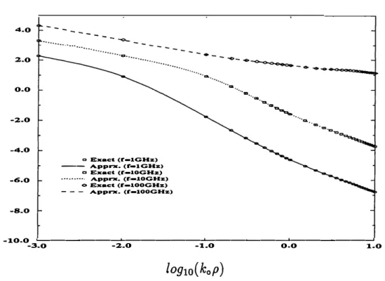
The assessment of the robustness of the proposed approach also requires a study

of the sensitivity of the approximation parameters to the geometrical constants and

the frequency. Hence the Green's functions for the vector and the scalar potentials

are obtained in closed forms for the same geometrical constants and for the same

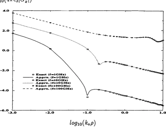
approximation parameters used above, but the frequency of operation is changed to

1 GHz, 10 GHz and 100 GHz. This is equivalent, in effect, to changing the geometrical

constants (see Figs. 10 and 1 1). It is observed that the agreements between the exact

20 M. I. Aksun & R. Mittra 4-0

r---�---�----�---�

···· .. ··· ··· ···_··· , .. m .. 2-0 -2.0 ·-..•.. ··-.. -1..0 - - E - c:t (GAxx) o A.pprx.(G.A.JilOc) ••••••••·· E,c:aclt (Cqx) Cl Apprx. (Gq:111;) '• ... .. al .. ,_{, 1D•·Cl•D} 1:1

Figure 8: The magnitude of the normalized Green's functions 41rG:.,/

µ

3 , 41rE3G� . 1st

layer- PEC; 2nd layer- E,2= 12.5, d2=0.03 cm; 3rd layer- E,3=2. 1 , d3=0.07 cm; 4th

layer- free-space, freq=30 GHz.

5-0 �----�---�----�---� ··, .. ··--...•.. ···--... .

_...

-- Exact. (GAzz.) o A.pprz. (G.A.zz) ... Exact (Gqz) .. A.pprx. (Gqiit) 0-0 '---�-,---.-.._,,----��---' -3.0 -2.0 -1-0 0.0 1.0

Figure 9: The magnitude of the normalized Green's functions 41rG1z/ µ3, 4u3G� . 1st

layer- PEC; 2nd layer- E,2= 12.5, d2=0.03 cm; 3rd layer- 1:,3=2. l , d3=0.07 cm; 4th

1 . Closed-Form Green's Functions . . . 2 1 4.0 -2.0 0.0 -2-0 -4.0 -6.0

- - -

--···•··· .,, Exact (l'-1GHz) -- A.pprx. (r-l GHz> a Exact (l'-10GHz) ··· ··· A.pprx. (l'-1.0GHz) o Exact (l'-lOOGHz) - - - .A.pprx. (l'-lOOGHz) ...

·­

......

---

...

"•c,,. . -10.0 �----�---�----�---� -3.0 -2.0 -1 .0 0.0 1.0

Figure 10: The magnitude of the normalized Green's function 41rG:,J µ3 • 1st layer­ PEC; 2nd layer- e,2= 12.5, d2=0.03 cm; 3rd layer- e,3=2. 1 , d3=0.07 cm; 4th layer­

free-space.

and approximate sets of data remain extremely good.

3. MoM Applications of the Closed-Form Green's Functions

After having introduced a robust and computationally efficient approach for the derivation of the closed-form Green's functions in the previous section, their use in the method of moments formulation is discussed in this section. Eliminating the Sommer­ feld integral in the application of the spatial-domain MoM results in two-dimensional integrals over finite ranges, and, consequently, the computational efficiency improves significantly. However, one still needs to evaluate the remaining double integrals numerically, which is the limiting factor for matrix-fill time in the application of the spatial-domain MoM for a printed geometry. In this section, we will demonstrate that the use of the complex exponentials in place of the spatial-domain Green's functions further improves the matrix-fill time because it facilitates the analytical evaluation of the remaining double integrals. Thus, a substantial improvement in the matrix-fill time is achieved by eliminating all of the numerical integrations involved in the ap­ plication of the spatial-domain MoM to the solution of the Mixed Potential Integral Equation.

22

M. I. Aksun & R. Mittra

4_0 ,---�----�---�----� 2.0 ··· ......... -.. ....._{... .}

---�

0.0 -2.0 -4.0 o Exac:t cr-1GHz> -- Apprx. cr- a GHz> 1:1 Exact (l'-.&OGHz> ... A.pp-. (C-J.OGHz) • Ex.et (f'-.&OOGHZ) - - - Apprx. (l'-J.OOGHz)

-6·0_3'-::.0:---�2.-=o---:_1�.o=---=-o"-=.o----�1.o

Figure 1 1 : The magnitude of the normalized Green's function

_41rE3

G�. 1st layer­

PEC; 2nd layer-

E,2

=12.5, d

2

=0.03 cm; 3rd layer-

E,3

=2. 1 , d

3

=0.07 cm; 4th layer­

free-space.

3.1 Formulation for the Spatial-Domain MoM

Before going into the details of how the closed-form Green's functions are employed

in the MoM formulations, it would be instructive to present the formulation for the

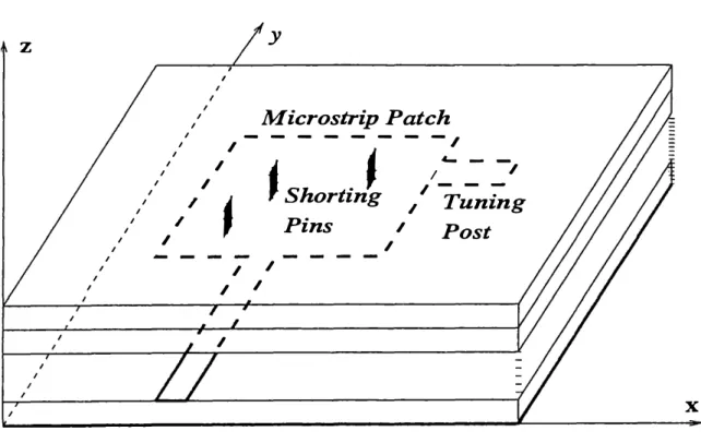
spatial-domain MoM for 2.5D geometries in a multilayer environment. For the sake of

illustration, a typical 2.5D geometry is depicted in Fig. 12 and the MoM formulation

is demonstrated for this geometry with no loss of generality. Note that the geometry is

multilayer and has vertical connections, e.g. , shorting pins, as well as two-dimensional

printed conductors. All of the layers and the ground plane are assumed to be infinitely

wide in the horizontal plane, and the conductors are assumed to be lossless and

infinitesimally thin.

The tangential components of the electric field on the plane of the patch and on

the shorting pins can be written in terms of the surface current density, J, and the

associated Green's functions as follows:

E

_,,

= -jwG:

_,,

* J

_,,

+

-;..-8

8

(G

q

_{• *- V · J)}

₍₄₀₎

J W X

E

_y

= -jwG�

_Y

* J

_y

+

-;..-8

8

(G

q

• * V · J)

(41 )

• _{J W y}

1 . Closed-Form Green's Functions . . . 23

z

, , , , , , , , , , , , , , , ,

y

:

Microstrip Patch

, , ,

/ - - - -/

/ / /

/

'

'

'

/

... -

-/

, Shorting / / T;;nbig

_Pins

/

_Post

/ / / / / /

Ground Plane

Figure 12: A typical 2.5D geometry in a multilayer medium. X

where * denotes convolution and G1., =G:_y· Gj re_Presents the i-directed vector po­ tential at r due to an j-directed electric dipole of unit strength located at r', while Gq• represents the scalar potential by a unit point charge associated with an electric dipole. Since the traditional form of the Green's functions are employed in the above formulation, the Green's function for the scalar potential is not unique for the HED and VED. Hence, the term involving the Green's function for the scalar potential, which is common in Eqs. (40) -(42), can be explicitly written as

8J

8J

8J

Q9•

*

'v . J

=

Q9•

_{"' 8x}

* -"'

+

Gq•

*

_Y

+

Gq•

*

_z

Y

8y

z

8z

where G't,e =Gi• for an HED and Gi• for an VED.

(43) To solve for the surface current density J via the MoM, J is expressed as a linear combination of the basis functions, which are chosen in this work to be rooftops for the x- and y-components and pulses or rooftops for the z-component of the current density (see Fig. 13) . Hence, the components of the current density are expressed as:

J:z:(x, y) = L L I!mnJntnl (x , y) (44) m _n Jy(x, y) =

I:I:

r!mn>ntni (x, y) (45) m _n Jz(x, y, z) = L I!'l Bi'l(x, y, z)

(46)

I

24 M. I. Aksun & R. Mittra

B (x,y)

_y

a

. .

Shorting

pin

Bz(x,y,z)

Figure 13: Basis functions representing the current density.

where B£mn) and B�mn) are rooftop functions, and

B£

1l is pulse or rooftop functions, !£mn) and I!mn) are the unknown coefficients of the basis functions at the (m, n)th position on the subdivided horizontal conductor, and I1'l on the /-th shorting pin or the via hole. One of the basis function can be considered as that associated with the current source, of course with a known coefficient.

Following the substitution of Eqs. ( 44)-( 46) into Eqs. ( 40)-( 42), the boundary conditions on the tangential electric fields on the conductors are applied in integral sense by testing the resulting equations with some testing functions, say TJm_{'n') ,} TJm'n') and TJ"l . This leads to a matrix equation for the unknown coefficients of the basis functions which reads

[ z(m'n' ,mn) :,::,: z(m'n' ,mn) y:i: z(l',mn) z:,;

[ Z ] [I ] = [

V

j

z(m'n' ,mn) z(m'n' ,I)

l [

J(m n)

l

:cy :cz :c z(m'n' ,mn) z(m'n' ,I) J(mn) yy yz y z(l',mn) z(l',I) J(I) zy zz z [ vJ m_'n')

l

=

v.:!m'n') v(I') _z (47) where

Zs

denote the mutual impedances between the testing and basis functions, and

Vs

represent the excitation voltages due to the current source. For the sake of brevity, the explicit forms of the impedances and voltages in Eq. (47) are not given here for this general case.

1 . Closed-Form Green's Functions . . . 25

3. 2 Closed-Form Green's Functions for MoM applications

In Section 2, a general procedure for deriving the closed-form Green's functions for the vector and scalar potentials was detailed. However, a discussion of the technique for rendering these closed-form expressions numerically efficient when they are used in conjunction with the method of moments was not included. As mentioned in Section 2.2, the terms in the square brackets in Eqs. (6)-(15) should be sampled uniformly along kzi and approximated in terms of complex exponentials. However, in order

to do this, it is necessary to fix the vertical coordinate variable z and apply the GP OF approximation technique anew for each value of

z.

For geometries involving horizontal conductors only, this would not be a computationally inefficient procedure because the conductors would be located at constant z-planes. As an example, for a microstrip line along the x-direction, the only MoM matrix element is z£7,;im_{'), and} can be written explicitly as;

( ') ( ') A ( ) 1 ( ')

8

aB(

m)

z,;;:m = < T,,m , G,,,, * B,,m > +_w2 < T,,m _{' 8x}[G!• * a: ] >

(48)

where

a:

_,,

and G!• used in this formulation are approximated by GPOF for constant

z's

corresponding to the planes of the conductors in the geometry. However, for geometries with both vertical and horizontal conductors that support both

z

and x-directed current components, typical MoM matrix elements have the forms

T(I')

G

A B(m) T(I')

!_[Gq· aBJ

m)

]

<

z 7 ZX

*

X

>,

<

_{Z >}

a

_z

X

* a

_x

>

<

r(I'> G

A

*

_B<'l

>

<

r(l'l !_[Gq·

*

8B1'l

i

>

z , zz z , z ,

a

_z

z

a

_z

(49)

where

<,

> and * denote inner product and convolution, respectively. G!, G1z, G!• and G'i• need to be approximated at every observation point

z,

and/or source point

z'

values in the integration due to the testing and expansion processes along a ver­ tical conductor. (Note that if we assume the origin is located at the bottom of the source layer for the application of the MoM, the coordinates used in the derivation of the Green's functions here can be transformed from

z

to

z

-

z',

and h to

z').

However, this would defeat the purpose of using the closed-form Green's functions in a MoM application. To circumvent the problem associated with the testing process, which corresponds to integration along

z,

the GPOF method can be applied to the complex coefficients of e±ik_,;z _{in all the Green's functions except}

a:/.

_{Hence, the} z-dependence in the closed-form Green's functions becomes explicit and the testing procedure along the z-direction can be performed analytically for some testing func­ tions like uniform and roof-top functions, which further improves the computational efficiency of using the closed-form Green's functions in conjunction with the method of moments.

Another technique, proposed herein, to overcome the above mentioned difficulties is to interchange the order of integration ( 49), provided that the basis and testing

26

M. I. Aksun & R. Mittro

functions are so chosen that the involved integrals a.re uniformly convergent37_{, a.nd} carrying out the integration over

z

analytically for spectral domain representation of the Green's function multiplied with the testing function. Next, the approxima­ tion method, GPOF, is applied to the resulting spectra.I domain function. For the inner product terms involving both the z and z' integrations, these integrals can be performed analytically by using the procedure described above, and subsequently ap­ plying the GPOF algorithm. Note that the spectral representations of the Green's functions are exponential functions of z and z', and this enables us to carry out the

z a.nd z' integrations analytically in the spectral domain. 3. 3 Analytical Evaluation of the MoM Matrix Elements

The formulation presented herein is a.pplica.ble to genera.I microstrip geometries in a multilayer medium where it is assumed that the layers extend to infinity in the transverse directions. However, to illustrate the main concept of the proposed method, the formulation is presented, without loss of generality, for a microstrip etch on a. substrate for which only the longitudinal current is assumed to exist. To calculate

Basis functions

...

Feed ::: : \

t

/-

z -/ I

d

E

_Substrate

t

Ground plane

Figure 14: A typical microstrip geometry. €r =4.0, d=0.02032 cm, f=l.0 GHz. the necessary Green's functions in a. closed-form, we consider the following para.meters for the geometry of a substrate ha.eked by a ground plane, (see Fig. 14) . The dielectric constant €r of the substrate is 4; the thickness of the substrate d=0.02032 cm; and, the frequency of operation f=l.0 GHz. The Green's function of the vector and scalar potentials due to an HED located a.t the air-substrate interface are obtained in closed forms via. the two-level approximation scheme, and the coefficients a1n , a_2n and the

exponents a1_{n, a}2_{n are given in Table 1 along with the normalized Green's functions}

for vector and scalar potentials, 47f"G:,,; µo and 47f"€oG!• , respectively, in Fig. 15. The mixed-potential integral equation for the microstrip line can be transformed into the

1. Closed-Form Green's Functions . . . 27 Table 1. Coefficients and Exponents for the closed-form Green's functions

41rG:

,,

/

µo

=

E�v,;i'4 Une-ik,rn /rn 471'€oG!•

=

E:�i'8 Une-ik,rn /rn

Un an Un an -1.0000+j0.0000 0.000+j0.0406 -0.590623+j0.0 0.0-j0. 103e-3 0.495e-6-j0. 123e-5 -0.0512+j0.0505 0.0196+j0.0374 0.0390+j0.0598 0.498e-6+j0. 123e-5 0.051Hj0.0506 -0.4485+j0.0 0.0+j0.0345 1.0+j0.0 0.0+jO.O 0.0196-j0.0374 -0.0390+j 0.0598 -0.260e-10+j0. 77le-l l -53.33+j439.67 0.279e-5-j0.245e-6 -0.3396+j 0.9239 0.204e-6+j0.328e-6 1.0270-j0.2907 l.O+j0.0 0.0+j 0.0

matrix equation via the spatial-domain MoM, and a typical matrix element is given below to help demonstrate the use of the formulation;

The first inner product of (50) is written explicitly as

<

Tjm_{'J , a:}

,, * Biml

>=

(50)

iv)

dxdyTjm_{'l (x, y)}

iv)

_dx'dy'G:

,,(x - x', y - y')Biml (x', y') (51) where DT and Ds denote the domains of the testing and basis functions, respectively, and the closed-form Green's function

a:

,,

is expressed as in (39). By changing the order of integration, the inner product can be written

j j du dv a:,,(u, v)j j dx dy Tjm'l (x, y) Bim_{l (x - u, y - v) (52)} where the inner double integral is a correlation function represented as TJm_{') ® BJ}m_l. As is well-known, the choice of the basis and testing functions are of great impor­ tance for the accuracy of the results and for the convergence of the matrix elements involved in the MoM3_{7• Since the formulation presented here requires the correla­}

tion function to be polynomial function, the choice of testing and basis functions is restricted to polynomial like functions. Therefore, we choose the rooftop functions, which are triangular functions in the longitudinal direction and uniform in the trans­ verse direction, as the basis and . testing functions. Half rooftop functions are also used to model the current density at the load and source terminals38_•

For the above choice of the basis and testing functions, the correlation function becomes