FOR SI0 :;H ASTI€
i Γ^'·«Ό#3'
S-yShciTTSD TO THS &£PAhTM£í4T OF COr^PUTER
ENGiNEERîNG AND îNFORwiATJOfî SO & C E
ATO THS ;HST:TjTS '?T‘ ,.'T: . ;Sc.'.’. !T .•.. ■:C· SC;ST:.T£;
Dir BÎLAb^îT УІЬЛѴЕЙЗПТ
.S'·., ; ' 'î ·Γ - Й-4.liv ^ iïÎ^Sï·; '^Μ,'ώΜϊ
BASED ON SPLITTINGS
FOR STOCHASTIC AUTOMATA NETWORKS
A THESIS
SUBMITTED TO THE DEPARTMENT OF COMPUTER ENGINEERING AND INFORMATION SCIENCE AND THE INSTITUTE OF ENGINEERING AND SCIENCE
OF BILKENT UNIVERSITY
IN PARTIAL FULFILLMENT OF THE REQUIREMENTS FOR THE DEGREE OF
MASTER OF SCIENCE
Bv
Ertugrul Uysal
June, 1997
'
for the degree of Master of Science.
Asst. Prof. Dr. Tuğrul Dayar(Principal Advisor)
I certify that I have read this thesis and that in rny opin ion it is fully adequate, in scope and in quality, as a thesis for the degree of Master of Science.
Assoc. Pi'of. /Dr. Cevdet .Avkanat
I certify that I have read this thesis and that in my opin ion it is fully adeciuate. in scope and in c[uality, as a thesis tor the degree of Master of Science.
Approved for the Institute of Engineering and Science:
A B S T R A C T
ITERATIVE METHODS BASED ON SPLITTINGS
FOR STOCHASTIC AU TOM ATA NETWORKS
M.S. in Computer Engineering and Information Science Supervisor: Asst. Prof. Dr. Tuğrul Dayar
June. 1997
This thesis presents iterative methods based on splittings (Jacobi, Gauss- Seidel. Successive Over Rela.xation) and their block versions for Stochastic Au
tomata Networks (SANs). These methods prove to be better than the power
method that has been used to solve SANs until recently. Through the help of three e.xamples we show that the time it takes to solve a system modeled as a S.AN is still substantial and it does not seem to be possible to solve sys tems with tens of millions of states on standard desktop workstations with the current state of technology. However, the SAN methodology enables one to solve much larger models than those could be solved by explicitly storing the global generator in the core of a target architecture especially if the generator is reasonablv dense.
Keywords: Markov processes; Stochastic automata networks; Tensor alge
ÖZET
Ertuğrul Uysal
Bilgisayar ve Enformatik Mühendisliği, Yüksek Lisans Tez Yöneticisi: Yrd. Doç. Dr. Tuğrul Dayar
Haziran, 1997
RASSAL ÖZDEVİNİMLİ AĞLAR İÇİN BÖLÜNME TAB.ANLI
İTER.ATİF YÖNTEM LER
Bu tezde Rassal Özdevinimli .Ağlar için bölünme tabanlı dolaylı yöntemler (.Jacobi, Gauss-Seidel, Succesive Over Relaxation) ve bunların blok çeşitleri geliştirilmiştir. Bu yöntemlerin, yakın zamana kadar Rassal Özdevinimli Ağları çözmekte kullanılan power yönteminden daha iyi oldukları gösterilmiştir. Uç örnek yardımıyla, Rassal Özdevinimli Ağlar kullanılarak geliştirilmiş bir mo delin çözülmesi için gerekli sürenin hala oldukça yüksek olduğunu, ve şu anki teknolojik imkanlarla, on milyonlar mertebesinde duruma (state) sahip bir modelin standart masaüstü bilgisayarlarla çözülmesinin pek mümkün gözükme diğini buluyoruz. Diğer taraftan Rassal Özdevinimli Ağlar yöntemi ile, tüm sis temi ifade eden matrisi bilgisayarın ana hafızasında seyrek şekilde saklayarak çözülebilecek modellerden çok daha büyük modellerin çözülebileceği görülmüş tür. Bu durum, özellikle tüm sistemi ifade eden matrisin yoğun olduğu du rumda geçerlidir.
Anahtar kelimeler. Markov süreçleri, Rassal özdevinimli ağlar, Tensör cebri.
A C K N O W L E D G M E N T S
The most I owe to my supervisor. Asst. Prof. Dr. Tuğrul Dayar for his guidance and support during this study. I would also like to thank my family for giving more than one can imagine, and all my friends including but not limited to Ertugrul Mescioğlu , Halit Yddirim, Kemal Civelek and Yusuf Vefalı, meeting whom has been and is going to be a source of happiness.
Finally. I would like to thank my committee members .Assoc. Prof. Dr. Cevdet Aykanat and Asst. Prof. Dr. Mustafa Pınar for their valuable com ments on mv thesis.
1 Introduction 1
2 Markov Chains 4
2.1 Preliminaries 4
2.2 Formal Definition of Markov C h a in s... 5 2.3 Discrete Time Markov C h a in s ... 8 2.4 Continuous Time Markov Chains 9 2.5 The Steady State Vector for a Markov C h a in ... 11 2.6 Methods for Numerically Solving Markov Chain Problems 14
2.6.1 An Overview 14
2.6.2 Power M ethod... 16 2.6.3 Methods Based on S plittings... 17
3 Stochastic Automata Networks 22
3.1 Preliminaries 22
3.2 Tensor A l g e b r a ... 23 3.2.1 Ordinary Tensor .Algebra... 23
3.2.2 Generalized Tensor A l g e b r a ... 25
3.3 Stochastic Automata Networks 27 3.4 Capturing the Interactions... 29
3.4.1 Functional T ra n sitio n s... 29
3.4.2 Synchronizing E ven ts... 30
3.5 Descriptor of a SAN 30 3.6 Efficient Tensor Product Vector M ultiplication... 34
4 Stationary Iterative Methods for a SAN 37 4.1 The splitting of a S.VN d e s c r ip to r ... 37
4.1.1 An Example Splitting 42 4.2 Iterative Methods Ba.sed on Splittings... 46
4.2.1 J a c o b i ... 46
4.2.2 Gauss-Seidel 47 4.2.3 Successive Overrelaxation 53 4.3 Block Methods 53 4.4 .An Upper Bound on S o lv e D -L ... -54
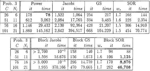
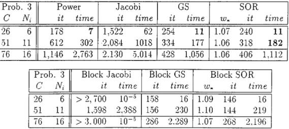
5 Numerical Results 57 5.1 The Problems and the E.xperiments... 57
5.2 The Resource Sharing P r o b l e m ... 60
5.3 The Three Queues P r o b l e m ... 62
6 Conclusion 68
A Incorporating a New Model To Peps 70
A .l Preliminaries 70
A .2 Generating the Text F i l e ... 71 A .2.1 Format of a Single M a t r i x ... 71 .A.2.2 Example M atrices... 73 .A.2.3 The Text File and Its Parts 74 .A.3 Evaluating Functional Entries in P e p s ... 76
2.1 .A transition probability matrix 9
2.2 .A time homogeneous discrete time Markov ch a in ... 9
2.3 .A transition rate m a t r i x ... 11
2.4 A time homogeneous continuous time Markov c h a i n ... 11
3.1 Vector multiplication with an ordinary tensor p r o d u c t... 35
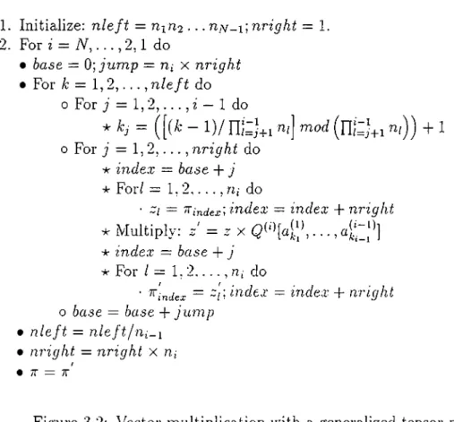
3.2 Vector multiplication with a generalized tensor p r o d u c t ... 36
4.1 Lower triangular part of Q \® Qz partitioned into blocks. . 49
4.2 The recursive lower triangular solution algorithm for SANs . . . 51
4.3 The Gaus,s-Seidel algorithm using S o lv e D -L ... 53
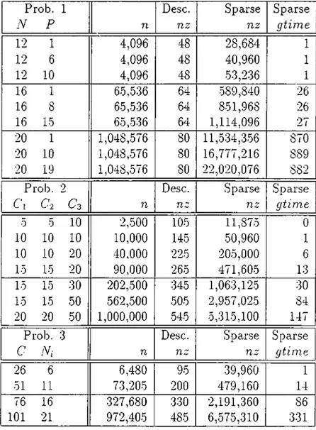
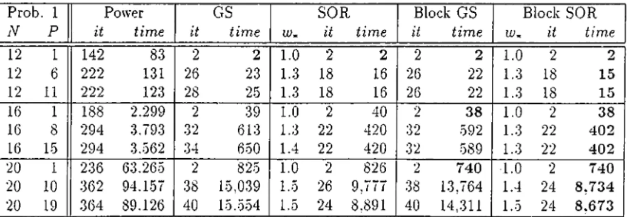
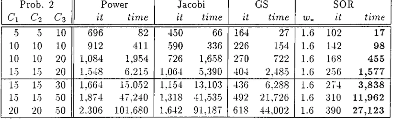
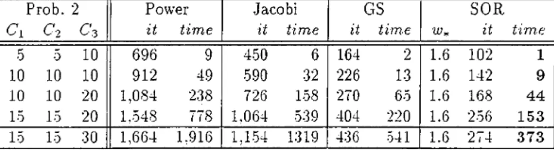
0.1 Storage Requirements and Generation Times for All Problems . .59 •0.2 Results of Desc. Experiments with the Resource Sharing Problem 61 ■0.3 Results of Sparse Experiments with the Resource Sharing Problem 61 •0.4 Results of Descriptor Experiments with the Three Queues Problem 62 ■0..0 Results of Sparse Experiments with the Three Queues Problem . 63 •0.6 Parameters for the Mass Storage Problem...64 •0.7 Results of Descriptor E.xperiments with the Mass Storage Problem 6-5 •5.8 Results of Sparse E.xperiments with the Mass Storage Problem . 66 •0.9 Results of Other Experiments with the Mass Storage Problem . 66
A .l Matrix Types
.A.2 Types of Nonzero V a lu e s ... 72
•A.3 Model Types 74
Introduction
Markov chains [16] are one of tlie most widely' used modeling technic[ues in the scientific community. The range of application domains is wide, including natural sciences and engineering disciplines. The simple requirement for a system to be modeled as a Markov chain is that the system’s next action (transition) depend only on the current state of the system, named as the
mtmoryless or the Markov property [16, p. 4]. Several natural phenomena
that arise in biology, physics and chemistry can be modeled as Markov chains. In engineering sciences Markov chains have a wide use in several branches of industrial engineering, electronics and computer engineering. Performance evaluation and reliability modeling is the field that Markov chains find the most use in computer engineering.
The random behavior of a system should posses a geometric or exponential probability distribution in order to be modeled as a Markov chain, since these are the only probability distributions that carry the memoryless property [16, p. 4]. Fortunately, the number of systems that show this structure is large and we have methods for fitting the random characteristics of most systems into e.xponential or geometric distributions.
After modeling a system as a Markov chain, one seeks quantitative informa tion from the built model. One attractive feature of Markov chain models is that most interesting properties of a Markov model can be obtained by solving
a linear system of equations. Much research result is available concerning the numerical solution of Markov chain models. In addition to this, interest in this field of research is still alive. Most methods for solving systems of linear equations may be used for Markov chain models effectively. Direct methods do not seem to be suitable for solving large and sparse systems which arise in
/
Markov chain models. Several types of iterative methods are applied to Markov chains and their properties in the context of Markov chain models are stud ied. However, much research needs to be done, for understanding the behavior of iterative methods, especially non-stationary iterative methods like GMRES and .Arnoldi[8].
In Markov chain applications, the problem size increases very quickly as the applications get more interesting. This problem is referred to as the state
space explosion[lQ, 14, 4] problem and has initiated different approaches to
the Markov chain problem. .Approximate solutions and bounds for the so lution vector[14] are studied for reducing the complexity of the problem. In plain words the coefficient matrix, constructed for solving the linear system of equations, becomes very large and prohibits one to solve interesting problems beyond a certain limit. Stochastic Automata Networks (SANs) [16. 10. 11] are developed to overcome the difficulties that accompany the state space explo sion problem. Although it is possible to apply SAN methodology to different domains, performance modeling of parallel and distributed computer systems are especially suited to this type of approach[5j. In SAN methodology, a system is modeled as a set of components interacting with each other. Characteris tics of each component is captured separately from the interactions among the components, and formulated in compact form, which leads to considerable re duction in the amount of storage needed for the model. Methods available for solving Markov chain problems obtained from a SAN formalism, appear in two forms. One might prefer to store the coefficient matrix of the linear system of equations in sparse format. However, this approach does not make use of the storage reduction provided by the SAN methodology. On the other hand, it is possible to solve the system by only referring to the compact storage of the model. Currently, the power method and non-stationary methods of GM RES and Arnoldi are implemented for SANs in compact form, but there are no results available concerning the solution of a real life problem obtained from
these methods[17, 6].
In this thesis, we introduce the concept of a splitting for a SAN in compact form and develop the stationary methods of Jacobi, Gauss-Seidel and SOR based on this splitting[16, 7]. We also implement these iterative methods based on splittings and their block versions. In addition to this, we e.xperiment with these methods on real life problems. We investigate the performance of these methods and their sparse counterparts compared to the power method.
In the following chapter, we introduce several concepts related to Markov chains and give the formulation of the problem of solving a Markov chain model as a linear system of equations. Stationary methods for Markov chain problems are also introduced in this chapter.
The third chapter discusses SANs. The concept of a SAN model in compact form is e.xplained with an example and the necessary algebraic framework for building SAN models is also provided. This chapter ends with an algorithm and a theorem regarding the complexity of the algorithm, that proves to be useful for SAN models in compact form.
The stationary iterative methods based on splittings for solving S.ANs in compact form are introduced in the following chapter. The algorithms provided for the methods are explained and a section on numerical results present the performance of the methods on three problems. Some interesting properties of block methods that have gone unnoticed so far are included in this chapter. An upper bound on the number of multiplications for the Gauss-Seidel and SOR methods are derived at the end of the chapter.
The last chapter contains conclusive remarks about the methods investi gated. Observations and comments about methods, the SAN methodology and Markov chains based on our work are provided in the chapter.
We included an appendix that describes how to incorporate new models into the Peps package[12], which is the software tool developed in France for solving S.AN models in compact form, since we implemented our methods as an extension to Peps.
Markov Chains
2.1
Preliminaries
In our attempt to understand the characteristics of natural and artificial phe nomena. mathematical models of systems are developed. It is possible to build models using the concept of the system being in a number of states. Generally, the system is thought to be in an initial state, and its behavior is modeled as transitions from one state to another. It is also possible to classify systems according to certain properties they might hold. One such property that the system modeled as a process changing states might have is the memoryless property, i.e., it only remembers its current state [16, p. 4]. In other words, the system’s transition from one state to the other is independent from the previous states that the system has visited.
In many of the models arising from diverse fields including natural sciences such as physics and biology, and engineering sciences such as industrial, elec trical and computer engineering, the system either has or can be modeled as having memoryless property [16, p. 3]. The systems that posses the memoryless property may be modeled as a Markov process [16, p. 4].
A system modeled as a Markov process has a number of possible states. The actual number of possible states can be infinite, however the system can be at only one of the possible states at any time instant [16, p. 4]. In addition
to this, it is assumed that the transition time, the time it takes the system to go from one state to the other is negligible. That is, the transitions are said to take place instantaneously. [16, p. 3]
It is possible to have a continuous state space for a Markov process. For instance, if the output voltage of an electric circuitry can take all values within a range, and if the system can be modeled as a Markov process, it can be modeled as a Markov process with a continuous state space, having the output voltage as states of the system. If, for instance, the circuitry’s output voltage raises from 0.6 volts to 3.7 volts, one would view the model as making a transition from state 0.6 to state 3.7. On the other hand, if the output voltage can take only certain potential values, and if the system can be modeled as a Markov process, the system can be modeled as a discrete state space Markov process. Note that the actual values of the voltages do not effect the discrete or continuous character of the system.
Markov processes with discrete state spaces are called Markov chains [16, p. 5], and they are what our work is based on.
In the ne.xt section, we give the definition of a Markov chain in a formal con- te.xt. The following two sections introduce two different types of Markov chains that arise in Markov chain modeling. Stationary distribution of a Markov chain[16. p. 15] is an important quantity for determining certain characteris tics of the model under consideration, and is introduced in the ne.xt section. Finally, methods developed for solving Markov chain models are discussed in the last section.
2.2
Formal Definition of Markov Chains
.A. Markov chain is a special case of a Markov process and, a Markov process is a stochastic process satisfying certain requirements. Hence, we give the def initions of stochastic processes in general, then Markov processes and Markov chains based on this.
D efin ition 2.2.1 [16, p. 4] A stochastic process is defined as a family o f ran
dom variables { X { t ) , t G T } defined on a given probability space indexed by the index parameter t, where t varies over some index set (parameter space) T.
In general, t takes values from the range (—o o ,+ c o ). In applications, the index set T is thought of as the set of time points at which observation about the system is made. In other words, the index t of the random variable is defined as the time point that X{ t ) takes the observed value. In such cases, t takes values from the range [0 ,+ o o ). Depending on the characteristics of the values t takes, the process is either a continuous parameter (time) stochastic process or a discrete parameter (time) stochastic process. If i can take discrete values only, or similarly, if obser^■ation about the system is made only certain equidistant time points, the process is called a discrete-time parameter process. If the range of values of t is [0, +cxo) without any restrictions, or the system is observed at time points that are not equidistant, the process is referred to as a continuous-time stochastic process.
D efin ition 2.2.2 Markov property: [16. p. 4] Let { X { t ) , t G T } be a stochastic
process defined on a given probability space indexed by the time index parameter t. where t varies over time index set T. Let the system be observed at time points to, t i . , . . . ,tn and let to < ti < . . . < The stochastic process {A ’ (f), i G T } is said to have the Markov property if and only if
Prob{ X{ t ) < x\X{to) = X o,A '(ii) = X i ,...,.Y ( i „ ) = ;i-„}
= Prob{ X{ t ) < a;|A^(i„) = x „ }.
In plain words, Markov property states that the next transition of the system from the current state X{tn) = Xn to the next state X { t ) = x, depends only on the current state X{ tn) = Xn and is independent of its previous state history, i.e., it is independent of the states A’(io) = 2:0, A ’(ti) = x \ ,... ,X ( t „ _ i ) = .r„_i. In other words, the current state of the process provides sufficient information to make the next transition.
D e fin itio n 2.2 .3 A Markov process is a stochastic process which satisfies the
For any stochastic process, and hence for any Markov process, the values that the random variables X { t ) take, define the state space of the process. As with the index set parameter t, the state space of a process can be continuous or discrete, finite or infinite.
D e fin itio n 2.2.4 .4 Markov chain is a Markov process whose state space is
discrete.
In Markov chain terminology, the state space of a chain is generally associated with the set of natural numbers. In other words the states are referred as state 0. state 1. etc.
When a stochastic process possesses a certain condition on the random variables and the index parameter (namely the Markov property), the process is said to be a Markov process. Similarly, the time index set and the state space characteristics of a Markov chain give rise to several types of Markov chains.
In a homogeneous Markov chain, the transitions of the system are indepen dent of the time parameter t. The Markov property requires that the next transition be independent of the previous state history of the process. How ever, it is possible that the proce.ss makes a transition which is dependent both on the current state of the system and the value of the time parameter t. Such a Markov chain, in which the transitions out of a state are dependent on the time parameter i, is called a non-homogeneous Markov Chain.
Similar to the state space of the process, the index set (the time parameter) can be continuous or discrete. If the time parameter of a chain takes its values from a discrete set, the Markov chain is called a Discrete Time Markov Chain (D TM C). If the values of t are are continuous, the Markov chain is called a Continuous Time Markov Chain (CTM C).
In summary, there are four parameters that describe a stochastic process. First, the continuous or discrete character of the state space, is a determining property of the process. Second, the continuous or discrete character of the time parameter introduce another classification dimension for the processes. Third,
the time homogeneity of the process, is also an important quantity, in capturing the properties of a process. Finally, the characteristics of the relations between the index set and and the random variables, i.e., the dependencies among them, define classes of stochastic processes. The classification that is determined by the character of the state space is important and is discussed in more detail in the following chapters.
2.3
Discrete Time Markov Chains
If the index set of the Markov chain is countable, i.e., it is in one to one cor respondence with the set of natural numbers, the Markov chain is called a Discrete Time Markov Chain. In this case, the index set is in general taken to be the set of natural numbers and the random variables are numbered accord ingly, i.e., as -Yo, A 'l,. . . , A „.
For a non-homogeneous Discrete Time Markov chain, the Markov property is described as [16, p. 5]
Prob{ An+i ^ ^n+i IAq .I’oi A j — X i , A . j i — Xn} Prob{ Ati.)-! ^ Xn-j-ilAji — ·
The conditional probability that the process makes a transition to a new state j , given that it is in current state i, is called the single step transition probability. It is expressed as [16, p. 5]
Pij{n) = Prob{A',t+i =j \ Xn = i}.
Note that since the Markov chain is a Discrete Time Markov chain, the state indices i and j are natural numbers.
For a homogeneous Markov chain, the next transition of the process is in dependent of the index parameter n. The single step transition probabilities are written as
Pij ~ Prob{A,i-t-l ~ ~ ^}·
The random variables A’„ should be geometrically distributed in order to satisfy the Markov property. In other words there is no other discrete probability
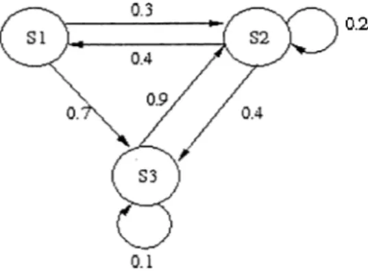
0 0.3 0.7 0.2 0.4 0.4 0.1 0.9 0
Figure 2.1: A transition probability matrix
0.2
Figure 2.2: A time homogeneous discrete time Markov chain
distribution that satisfy the Markov property. A homogeneous Discrete Time Markov chain's behavior can be e.xpressed as a transition probability matrix. Such a matrix is also called a chain matrix and is formed by putting the transition probability from state i to state j to the ith row and jth column of the matrix. Since the sum of the probabilities of making a transition from a state to all other states is one, the sum of the elements in any row is one. Such a matrix in which the sum of elements in any row add up to one is called a
stochastic matrix. In Markov chain literature, the transition probability matrix
is labeled P. Figure 2.1 demonstrates a transition probability matri.x of a homogeneous discrete time Markov chain with three states, that is described in Figure 2.2 with transition state diagrams.
2.4
Continuous Time Markov Chains
When the time indices of a Markov chain is continuous, the chain is called a Continuous Time Markov Chain. Note that, as in the case of DTMC, the state space is still discrete. In other words, the random variables describing the process might take discrete values; however the system might be observed,
i.e., make transitions, at any instant in time.
The Markov property for a non-homogeneous Continuous Time Markov Chain is expressed as [16, p. 17]
P rob {A '(i„+ i) < Xn+i \ X{ t o) = x o , X { t i ) = X u · . . ,X ( i „ ) = Xn}
= P rob{A '(i) < x\X{tn) = for any sequence of time points to < t\ < . . . < tn <
tn+i-The transition probability of a non-homogeneous CTMC is given by
= P rob {A '(0 = j\X{s) = ?}, for t > s.
Ill the homogeneous case, since the probabilities are independent of the ac tual values of s and t, the transition probability is expressed in terms of the difference t = {t — s), i.e.,
p ,j(r) = P r o b { X( s + r) = i|A'(s) = i}.
Ill this case a single probability transition matrix is not sufficient to express the behavior of the matrix, we need a set of matrices parameterized by r. Instead, a new matrix, called the transition rate matrix or the infinitesimal
generator matrix, is introduced. The matrix is constructed in a similar way
and is generally labeled Q. Yet, this time the enfries are not probabilities of making a transition from one state to another, but each element at row
i, column j of the matrix denotes an instantaneous transition rate. That is,
the entries of the generator matri.x are given by the rate of making transitions from state i to state j , when r is chosen to be sufficiently small so that the probability of observing more than one transition within the observation period
T is negligible. .A. more rigorous derivation of the rate matrix from the transition
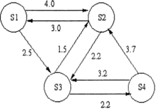
probabilities can be found in [16. p. 18]. In Figure 2.4 a CTM C is shown as a state diagram. Figure 2.3 gives the corresponding infinitesimal generator matrix. Note that the diagonal entries in each row are equal to the negative of the sum of the off-diagonal entries, i.e.,
Qij-—6.5 4.0 2.5 0 3.0 -8 .9 2.2 3.7 0 1.5 -3 .7 2.2 0 3.7 3.2 -6 .9
Figure 2.3; A transition rate matrix
Figure 2.4: A time homogeneous continuous time Markov chain
This can easily be understood if one notices that the entries are rates repre senting transitions from a state to others. The transitions from one state to itself (the rate at which the process stays at that state) will decrease as the rates to the other states increase. In [16. p. 19] this property of an infinitesimal generator matrix is also derived from the transition probabilities.
For a CTMC. the random variables X { t ) should be exponentially distributed in order to satisfy the Markov property. Similar to the discrete case, this means that no other continuous probability distribution satisfy the memoryless property.
2.5
The Steady State Vector for a Markov
Chain
The aim of modeling a system as a Markov chain, is to obtain some quantitative measures about the system. The information sought is mostly related to the states of the system. We wonder the states at which the system stays the most.
how long the system occupies certain states in the long run, etc. Depending on the system being modeled, one might be interested in some states of the system more than the others. Also, in general, the states of a Markov chain are classified into several groups and determining to which group a state belongs might be of interest, see [16, p. 8]. Specifically, a transient state is one which the system might not return back, in the long run. A recurrent state is one which the system is guaranteed to return after a number of transitions. In a Markov chain, it is possible that the process makes a transition to one state, and can not leave that state, i.e., there are transitions to that state but there are not any transitions out of the state. Such states are referred to as absorbing states. In practice, one is more interested in states that have some desirable or undesirable properties. Thus, one might wonder the probabilities of being ¿it those states or the average time the system spends at those states, in the long run.
It is suitable to express the state of a Markov model as a probability vector. A row vector tt is used with each entry i denoting the probability of being at
state i. When the system’s behavior is captured as a transition rate matrix Q or a transition probability matrix P, the properties of the Markov chain can be expressed as a simple set of linear ecpiations.
Now we introduce two important quantities that have desirable properties in the sense that they answer or provide the necessary information to answer several questions sought from a Markov chain model.
D e fin itio n 2.5.1 Limiting Distribution of a DTAIC :[16, p. 15] Given an ini
tial probability distribution 7t(0), if the limit lim 7r(n)
n—*co
exists, then this limit is called the limiting distribution, and we write
7T = lim 7r(n)
D efin ition 2.5.2 Limiting Distribution o f a CTMC iGiven an initial proba
bility distribution 7t(0), if the limit
lim irit)
exists, then this limit is called the limiting distribution, and -we write
7T = lim 7r(i)
f—CO ^ '
D e fin itio n 2.5.3 Stationary Distribution o f a DTM C :[16, p. 15] Let P be the
transition probability matrix o f a DTAIC, and let the vector z whose elements Zj denote the probability of being in state j be a probability distribution; i.e.,
G ^ Zj ^ 1, and 'y ' Zj = 1.
all j
Then z is said to be a stationary distribution if and only if zP — z.
D efin ition 2.5.4 Stationary Distribution o f a CTMC : Let Q be the transition
rate matrix o f a CTMC. and let the vector z whose elements Zj denote the probability o f being in state j be a probability distribution; i.e.,
Zj G 7^, 0 < < 1, and ^ = 1.
all j
Then z is said to be a stationary distribution if and only if zQ = 0.
For a certain class of Markov chains, (see [16, pp. 15-16]), if the limiting distribution exists, it is equivalent to the stationary distribution. Furthermore it is independent of the initial distribution, i.e., in the long run the effects of the initial distribution disappears.
The popularity and power of the Markov chain modeling paradigm comes from the fact that, most of the interesting properties of the system being mod eled can be derived from a set of simple linear equations. In the discrete case, the equations
wP = 7T, II 7T ||i= 1,
and in the continuous case, the equations
tQ = 0, II 7t ||i= 1,
Also the reformulation of the equation ttP = tt, as 7t( J — P ) = 0 show that
the problem of finding the stationary distribution of a discrete-time Markov chain, can be viewed as similar to a continuous-time problem. Conversely, a matrix P can be obtained from Q by
1 P = / + A tQ , where A t <
max I g,·,· I
The problem of finding the stationary distribution of a Markov chain can be thus formulated in three ways. First, it can be seen as an eigenvalue problem, i.e., 7tP = 7t; second, it can be formulated as a null space problem, i.e., kQ = 0:
and finally, it can be seen as a linear system that can be obtained in a variet\· of ways, from ~Q = 0, || tt ||i= 1.
VVe conclude this section by noting that all the discussed formulations of the problem imply that the Markov chains involved are time homogeneous, and this will be our assumption in the rest of the thesis.
2.6
Methods for Numerically Solving Markov
Chain Problems
2.6.1
A n Overview
-As the problem described in the previous section can be formulated in different ways, there are a large number of methods one may use to attack the problem. In general terms, direct methods refer to those methods that calculate the so lution vector in a predetermined number of steps [16, p. 61]. Iterative methods are provided with an initial approximation to the solution and they compute a new approximation to the new solution using the previous approximation in the previous iteration. The new approximation is supposed to become more and more close to the actual solution at each step.
Direct methods applied to Markov chain problems include Gaussian elim ination and LU decomposition. We note that in the case of a Markov chain
problem, a nontrivial solution other than the zero vector, to the system wQ = 0 is always available since it can be verified that Q is singular [16, p. 71].
Iterative methods can be grouped into two. First group of methods referred to as stationary methods include the power method, the method of Jacobi, the method of Gauss-Seidel and Successive Overrelaxation (SOR). The second group of methods are non-stationary methods, also referred to as Krylov sub space methods, include the method of Arnold!, Generalized Minimum Residual Method (GMRES) and the full orthogonalization method [16, pp. 117-230], [13]. In this work we concentrate on stationary iterative methods. Here we first give a comparison of direct and iterative methods in the conte.xt of Markov chains [16, pp. 61-62].
The value of a Markov chain model increases as the system being modeled becomes more and more complex. The increase in the complexity of the model is generally reflected as an increase in the number of the states of the Markov- model. This phenomenon is referred to as the state-space explosion problem. The increase in the number of states results in an increase in the size of the generator matrix. Beyond a certain limit, it becomes necessary to use a sparse storage scheme for storing the infinitesimal generator matrix. In addition to this, the matrices arising in Markov chain models are sparse, i.e., they contain only a few entries in each row. It is basically because of this reason that direct methods are considered disadvantageous, when compared to iterative solution techniques. Direct methods usually involve introducing new nonzero elements (fill-ins) into the matrix during factorization, which makes them inefficient and diflficult to deal with. Also, beyond a certain limit, especially for large problems, it might not be possible to store the newly altered matrix in core memory. In contrast, iterative methods involve only matrix-vector multiplications or equivalent operations, which do not alter the nonzero structure of the matrix. In addition to this, by not altering the matrix, we avoid the round-off errors which are observed in direct methods.
In certain cases, it might not be necessary to compute the stationary vector of a Markov chain, to high accuracy. In such uses, iterative methods allow one to stop the computation at a predefined error term.
On the other hand, iterative methods are usually accompanied with a slow convergence rate to the solution. It is this reason that one may use a direct method for Markov chain problems whenever the method is not limited im- practically by memory constraints. However, iterative methods ai'e still the dominant choice, unless a practically implementable direct method gives the solution in less time.
Stationary methods have been the subject of much research. Although the non-stationary methods seem promising, much research needs to be done on their convergence properties and to predict the number of iterations recjuired to find the solution of a problem. In the following sections we introduce the power method, method of .Jacobi, Gauss-Seidel and SOR.
2.6.2
Power Method
The power method is used to find the right-hand eigenvector of an ordinary matri.x corresponding to a dominant eigenvalue of the matrix. Thus, when the Markov chain problem is formulated as one of an eigenvalue problem, i.e.,
irP = 7T, power method might be used to solve the problem. Let the initial probability distribution among the states of a Markov chain be 7t(0), and let the probability transition matrix of the same chain be P. Then after the process makes a transition, (at the next step), the probability distribution becomes At the second step the probability distribution becomes
7t(2) _ 7r(i)/3 = Tr^°'>P'^. At the step, the probability distribution is found by TrP’l = Note that, is the new approximation to the solution at step k. For certain classes of Markov chains [16, p. 16], the vector tt**·'! approaches to the stationary distribution, i.e.,
lim = 7T, where tt --- ttP. k—roo
Power method is multiplying the approximation at each iteration by the prob ability transition matrix P , to obtain a new approximation. The convergence of power method is in general slow. Further properties of the method in the context of Markov chains can be found in [16, pp. 121-125].
2.6.3
Methods Based on Splittings
The stationary methods based on splittings are used for solving a system of linear equations. In the Markov chain context, when the problem is formulated as a linear system or a null-space problem, i.e., ttQ = 0, these methods may be
used. The methods .Jacobi, Gauss-Seidel (GS) and SOR are based on splitting the infinitesimal generator matrix Q into D — L — U where D is a, strictly diagonal matrix, T is a strictly lower triangular matrix, and U is a strictly upper triangular matrix. The matrix D consists of the diagonal elements of Q, and the matrices L and U consist of negative of the strictly lower and strictly upper triangular elements of Q. respectively.
The Method of Jacobi
The problem of .solving nQ = 0 can be formulated as
tQ = 0 k{ D - L - U ) = 0
ttD = Tr{L + U).
From this we can obtain the iteration matri.x of the Jacobi and the method of Jacobi
Hence, the method of Jacobi is equivalent to power method with the iteration matrix being (L + U)D~^.
The Method of Gauss-Seidel
In a similar way to the method of Jacobi, the Gauss-Seidel method can be derived from the formulation
ttQ = 0
t{ D - U ) = ttL
7T = ttL { D - U ) - K
From this we obtain the Gauss-Seidel Method as
Hence, it is eciuivalent to power method with the iteration matrix being
L( D — U)~^. The above formulation of the Gauss-Seidel method is referred
as a forward Gauss-Seidel, because when the equations regarding individual entries of the vector are considered, the elements are calculated starting from the first element to the last element of the vector
Another formulation is possible, which may be expressed as
In this case the order ol solving the equations for individual entries is from the last element to the first element of the vector ttG'+i). Hence the method is called a backward Gauss-Seidel.
The Gauss-Seidel method is different from the method of Jacobi as it makes use of the elements that have already been computed. For instance while calculating the ith element of the [k + l)st approximation vector it makes use of the first ¿ — 1 elements that have been computed so far, in the case of forward Gauss-Seidel. .A backward Gauss-Seidel makes use of the previously computed n — i elements ranging from index f -|- 1 to n, for a vector of size n, while calculating the ¿th element.
Successive Overrelaxation
The method of Successive Overrelaxation (SOR) is an extrapolation on the solution of the Gauss-Seidel. A parameter w is introduced to weigh the solution vector obtained from a Gauss-Seidel iteration with the previous approximation vector. When considered in this manner, the method can be expressed as
where is the resulting vector after applying the Gauss-Seidel algorithm to the ¿th approximation vector of SOR. Note that SOR is also called a forward SOR when the Gauss-Seidel iteration involved is a forward Gauss-Seidel, and a backward SOR when the Gauss-Seidel iteration involved is a backward Gauss- Seidel.
Hence forward SOR in matrix notation is
^(A:+l) ^ (1 - -t-U;(7r'^U^(r> - L)~^),
and backward SOR in matrix notation IS
Note that an SOR iteration with lu = 1 is equivalent to a Gauss-Seidel itera tion. Sometimes SOR. is referred as Successive Under Relaxation method when 0 < IÜ < 1.
In addition to forward and backward versions of SOR, a Symmetric SOR (SSOR) hcis been introduced, which is simply a forward SOR followed by a backward SOR. In the case of Markov chain problems, there is little benefit in using a SSOR instead of SOR and this can be observed only in rare examples [16, p. 132].
Convergence characteristics of stationary methods in a general context can be found in [7] and references therein. In the Markov chain context, [16, pp. 133-176], [4, pp. 125-132] and [1, pp. 26-28] [16, pp. 138-142] provide discussions of these and other methods.
Block Versions of Iterative Methods Based on Splittings
Stationary block iterative methods are based on block partitioning of the gen erator matrix Q. Following [16, p. 139] we can demonstrate a block partitioning
of the vector tt and the matrix Q as
(tTi, 7T2, · · · ? ^yv) )
Qll
Q
i2
Q
inQ21
Q22
Q2N
Q
niQ
nnIn this case, a block splitting of Q can be obtained as Q = (D¡^ — — D\
takes the form of a block diagonal matrix, L¡\r takes the form of a strictly lower block triangular matrix and I7/v is a strictly upper block triangular matrix, i.e..
D x =
Dn
0
0
0
D22
0
0
0
0
0
0
Uv2
Lxx
Lx =
Lzi
0
0
•
Lx =
0
0
H x-ix
Lxi
L.x v-i
0
0
0
By defining as the ith portion of tt as shown, we may define block Jacobi as
„ p + ll ^ ^
j = l j = ! + l
forward block Gauss-Seidel as
.G+l) _ N
x r “ = -, E for alH.
i = l j = i + l
and backward block Gauss-Seidel as
N i-1
7T
p +‘ l = E í-'iúiDu - E i r i ) · ' for- all i.j= i+ l i = l
The difference between the point and the block versions of the algorithms is that in the block versions, all elements of in a portion of are solved simultaneously. It is possible to use a direct method or another iterative
method to solve the individual blocks. In this way, one can obtain a more accurate approximation at each iteration, obviously with an extra cost being introduced at each iteration. In [1, pp. 26-28] block iterative methods are discussed within the context of Markov chains.
Stochastic Automata Networks
3.1
Preliminaries
In the previous chapter we have seen that if a Markov chain model of a system is available, qiuintitative measures about the system can be obtained from the system of equations
ttQ = 0, II ;r ||i= 1.
There are a number of methodologies for developing a Markov chain model of a system. Petri nets [8] are such a formalism for generating Markov chain models of systems. Alternatively, there are special software tools for generating Markov chain models [15]. Independent of the paradigm used, the problem of state-space e.xplosion is observed in almost all applications. In some cases, as the applications become more interesting, the size of the Markov chain gets so large that it is impractical to find a solution.
A Stochastic Automata Network (SAN) is another formalism for generating a Markov model. They are most suitable for performance modeling of parallel and distributed systems. The model is generated by considering an individual automaton for each component of the system. Each individual component is modeled by a single stochastic automaton and the interactions between the components are incorporated into the model. The main advantage of the SAN
methodology is that the model is stored very efficiently, i.e., the memory occu pied by the model is very small compared to the size of the model generated.
Before getting into the formal definitions of SANs and their properties, we give a basic overview of tensor algebra which is a building block for SAN methodology.
3.2
Tensor Algebra
3.2.1
Ordinary Tensor Algebra
We now list several definitions regarding tensor algebra. These and morere prop erties of tensor algebra concepts can be found in [2].
In the following, we use Amxn for a matrix of dimension m x n, B^t for a matrix of dimension k x 1. Cmkxni and Dmkxni for matrices of size mk x nl.
D efin ition 3.2.1 Ordinary Tensor Product:(OTP) Let A„i„ and Bki he two
matrices, as h\\ b\i A = an ^Ir ,B = hki hki
then the ordinary tensor product of A and B , Cmk ni = A Q B is given by
aiiB o-inB
c = \ ;
^ml-B . . . a^mnB
and the ordinary tensor product o f B and A, Dmk ni = B 0 A is given by h\\A . . . hiiA
D = '
Notice that C ^ D.
D e fin itio n 3.2.2 Ordinanj Tensor Sum: The tensor sum o f two square ma-
trzcei> A.JIJ2. nncl EjTiTTij Ctjiyji, titti — A. B zs defined us
C = A ® I m + I n
Further important properties of tensor algebra as they appear in [5, pp. 4-5] are listed below. Note that all matrices are square.
• Associativity ;
.4 0 { B 0 C) = {A 0 B) 0 C) and .4 0 (B 0 C) = (.4 0 .B) 0 C ). • Distributivity over ordinary matri.x addition :
(.4 + B )0 { C + D) = A 0 C + B 0 C + A0 D + B e D.
• Compatibility with ordinary matrix multiplication :(case I)
(.4 X B) 0 { C X D) = { A0 C) X {B 0 D).
• Compatibility with ordinary matrix multiplication :(case II) N (g) = n ^«1 ® ® ^n._. 0 0 0 . . . 0 /, ¿=1 ¿=1 N = n 0 AS'^ 0 /¿ + 1;/V, ¿=1
where Ii-j is the identity matrix of size Y[i=ink· • Compatibility with ordinary matrix inversion : (A X = 4 - 1 0 B ~ \
• Pseudo Commutativity : A 0 B = P r{B 0 A )P ^,
where Pr is a permutation matrix of order Ui x U2, nj is the size of matrix A and rin is the size of matrix B.
Note that no commutativity other than the given pseudo commutativity property holds for ordinary tensor products.
It is straightforward to extend these properties to N term tensor products and sums. For our purpose of illustrating several algorithms, noting that
N N
(g) ^ 0 . . . 0 0 A^^^ 0 0 . . . 0
k = l k = l
where /„^ is defined to be the identity matrix of size Uk which is the size of the term of the ten.sor product , A^^K is sufficient.
3.2.2
Generalized Tensor Algebra
Ordinary tensor algebra is used in other Helds of science as well as SAN mod eling. However, it does not allow one to handle certain constructs that arise in S.AN models. Since such constructs are essential for any meaningful model, tensor algebra has been extended in order to cope with them. Generalized ten sor algebra refers to tensor algebra where the elements of the matrices may be real valued functions. In SAN context, the functional elements are functions of the states of one or more automata. W e now give several definitions and properties of generalized tensor algebra. These with more detailed discussions and proofs can be found in [5, pp. 13-20]. VVe follow the conventions there and assume that all matrices are square, which is the case for us. A matrix of the form B[A] refers to a functional matrix B which contains entries that are dependent on the state of automata with transition rate matrix A. In general an expression of the form denotes a matrix
that contain functional entries that depend on the states of the automata . . . , Note that the state of an automaton is determined by the row of the generator matrix, i.e.. elements on row i of the matrix are transition rates out of state i, except of course the diagonal element which is interpreted as the rate of staying in the same state. The operator 0 ^ is used for generalized tensor products.
D e fin itio n 3 .2 .3 Generalized Tensor Product:(GTP Gase I) Let A and B[A\
he two square matrices with sizes and respectively, and let B contain functional entries that depend on the state o f A. Then the generalized tensor
product of A and B , C — A ® g B[A] is given by ацВ{ аі ) ai2B{ ai ) a2lB(^a2) *^22-^(^2) ^Па1-®(^Па) ^Па2-^(^^По) α ι„„β (α ι) α2πα^(«2) ^ПаПа^і^Па )
D efin ition 3 .2 .4 Generalized Tensor Product:(Case II) Let A[B] and B be
two square matrices with sizes n, and ni, respectively, and let A contain func tional entries that depend on the state o f B . Then the generalized tensor prod uct o f A and B . C = A[B] Ag B is given by
ап[В]Іпь
X B
ar¿[B]Inb
x B
U2i[B]Inb
X B
а22[В]Іпь
X B
аіпа[В]Іпь X B ^-^'ína\B\In|, X B
^^ncil\B\Ini, X B ana2[-^]-^il(, X B ^nanc\B\In,, X B
where aij[B\In^ is defined as diag{aij{bl),aij{b2) , . . . ,aij(bnb)} and aij{bk) is the functional element o f A with its function being evaluated at state k o f B.
D efin ition 3.2.5 Generalized Tensor Product:(Case III) Let A[B] and B[A]
be two square matrices with sizes Па and щ respectively, and let A contain functional entries that depend on the state o f B. Let B also contain functional entries that depend on the state of A. Then the generalized tensor product of A and B, C = A[B\ 0 g B[A] is given by
ап[В]Іщ X B(ai) au[B]Kt, x B{ ai ) й2і[В]Іщ X B{a2) а22[В]Іщ x B{a2)
^^lna[B]In^, X В{^йі)
а2па[В]Іпь X В{а2)
0'Паі\.В\Ігц, X В { ап а ) ^Па2[В]Іп(, X В{^СІп^) ^^nana\B\In^, X Bi^ünf)
where aij[B]I^ and aij{bk) are defined as in case II.
Now let us see some of the properties of generalized tensor algebra that are of interest to us.
• Associativity :
• Distributivity over ordinary matrix addition :
(Ai[5] + Ao[B]) 0 , {B,[A\ + B2[A]) =
A\[B\ ®g -6l[A] + A\[B] ®g + ^2[-5] ®g B\[A\ + A\[B] 0g B2\A\.
Compatibility with ordinary matrix multiplication :
0 , 0 , ^(2)] 0 , .. . 0 , . . . , >lbv-i)] h : N - i ® g I\:N--2 ®g A^^ . . . , 0 j In:N X /i:.V-3 0 , . . . , 0 , X X h : l Zg A^^^[ A^^^] 0g K y X .4^^* Z g Z g h - . N • Pseudo Commutativity : N N j /l=1 9 ^’=1
where r is a permutation of integers [1,2, . . . , jV], and Pr is a permutation matrix of order [li^i ^i·
3.3
Stochastic Automata Networks
Let us consider two stochastic automata initially without any interaction among them. The system being modeled has two components, each of which can be represented by a single automaton. A Stochastic Automata Network, describ ing the system, is represented by two automata, If the automata are models obtained from DTMCs, i.e., they are defined by probability tran sition matrices P^^^ and the whole system is defined by the transition probability matrix obtained from a tensor product, i.e., © P^^^ On the other hand if the automata are models obtained from a CTMC, i.e., have transition rate matrices and Q^'^\ the transition rate matrix of the whole system is obtained from the tensor sum of and as If
the probability distribution of the states of the first automaton at time i, is represented by vector 7r(^^(i), and similarly if the probability distribution of the second automaton are represented by 7г(^)(í) at time i, the probability distribution describing the state of the whole system at time t, is given by
0 7гf^^(í). If the first automaton has rii states and the second automaton has U2 states, the whole system has rii x ri2 states. Each state of the global
system is a combination of the states of the two automata. The global state of the system can be represented by a 2-tuple, i.e., if the first automtiton is at state i. and the second automaton is at state j , the global system is at state
(i. j)· It easily verified that each row of the global generator matri.x and the global state distribution vector corresponds to a state of the global system represented as a 2-tuple. A consequence of these results is that the stationary distribution of the global system can be obtained from the tensor product of the stationary vectors of the individual automata. Hence, it is straightforward to find the stationary vector of a SAN with noninteracting automata, i.e, first solve for the stationary vectors of the individual automata then calculate the tensor product ol them.
In case the global system is modeled by N automata. the global generator is obtained by
N
0 = © «''■ >
¿=1
in the continuous case, and by
P =
t = l
in the discrete case.
In both cases the global state distribution vector is obtained by
7r(t) =
¿=1
3.4
Capturing the Interactions
3.4.1
Functional Transitions
In order to be able to model complex systems, especially parallel and dis tributed systems that have interacting components, one needs to model the intei'ciction between the components. One extension that enables us to incorpo rate such interactions between individual components is by means of functional
transitions. The stochastic automaton, modeling a component, is allowed to
have transitions whose rate is a function of the states of several automata. Now, the entries of the transition rate matrix might be functional, i.e., the transition rate matrix is not an ordinary real valued matrix but it is a matrix whose entries may contain a real valued function. Note that if the rate of a transition is dependent only on the automaton that makes the transition, the transition is considered to be a constant transition, not a functional one.
Similar to noninteracting automata, the global generator matrix of the global system composed of CTiVtC can be described as a tensor sum of the generator matrices of the individual automata, yet this time as a generalized tensor sum of the individual matrices, i.e.,
<?= Ф
i'=l g
In the discrete case a generalized tensor product is needed, i.e.,
N P = p(i)
!=1 g
Two important points to note about functional transitions in SAN descrip tors is that; first, still the transitions of an automaton effect only the automaton itself even if the transition is a functional one, second, the nonzero structure of the generator matrix is still in a suitable form to store in sparse format, i.e., no zero entry may become nonzero during function evaluation yet some nonzero entries might evaluate to zero.
3.4.2 Synchronizing Events
Another concept, introduced to extend the modeling capability of a stochastic automata network, is one of a synchronizing event. A synchronizing event is either a transition of one automaton that force one or more automata to spe cific states, or an event in which an automaton being (or not being) in a state force some other automata to get into or stuck at certain states. The transi tions that are involved in a synchronizing event may also contain functional rates. It is possible to have a synchronizing event in which a transition of an automaton cause several or all automata to make or block transitions. Note that, a synchronizing event causes the state of the global system to be altered, whereas a functional transition affects only the automaton that contains the transition.
In .SAN terminology, the automaton that initiates a transition in the other automata in a synchronizing event is called the master automaton of the syn chronizing event. The automata that are effected by the master automaton’s transition are called the slave automata. Note that a transition in the master automaton has a rate associated with it, whereas the induced transitions in the slaves happen instantaneously with the master automaton's trcinsition.
3.5
Descriptor of a SAN
In this section we introduce the concept of a descriptor for a SAN. Plere and hereafter, we consider only continuous-time stochastic automata and hence all matrices are transition rate matrices. The extension of the concepts introduced, to discrete-time automata are possible. The effect of a synchronizing event on a SAN is captured by introducing new tensor product expressions. If there is a synchronizing event labeled e that appears in a SAN with N automata, one new tensor product of the form
N
1=1
and another one in the form
0 Q i ‘ >
2 = 1
are introduced. The last term is referred to as the diagonal corrector of the synchronizing event and is introduced to maintain the global generator as a transition rate matri.x:. In the most general case, where the transitions in volved in the synchronizing event, say e,·, are functional, the tensor products are generalized tensor products and the expressions introduced are in the forms
^ ¿=1
and
N
■7 1=1
For a SAN model with N automata, there are N matrices in the tensor products, each of which correspond to one automaton in the SAN. For each synchronizing event, the order of the terms in each tensor product are explicit as described bv
and
Q i" 0 , 0, . . . 0, e r >
0 , Ql"’ 0j . . . 0j O f * .
This is important since neither ordinary nor generalized tensor products are commutative.
Since for each synchronizing event, two new tensor products are introduced, for a SAN model with E synchronizing events, 2E tensor products are intro duced. The global generator of a SAN with iV automata and E synchronizing events is obtained from the equation
N ^ ^ Q = © « « + E © O f+ E<J? 9 i=i 1=1 9 i=l j = l N 2E = E ^-1 ® ® ^«.-1 ® ® ^".+1 1=1 N+2E • · 0 iriN + ^ (g ) Qj(¿)
= E ® <55
J=1 9 i=iand the form of it as in the last line is referred to as the descriptor of the SAN. The first set of N tensor products are referred to as the local generator matrices, the E tensor products of the form are referred as the synchro-nizing event matrices, the final tensor products of the form J2f - i g
are referred as the corrector matrices. The synchronizing event matrices reflect the interaction among the automata involved in the event. The corrector ma trices are diagonal matrices introduced to make the global generator matrix a transition rate matrix. Further information about the rationale behind these matrices with the related proofs might be found in [9], [10], [11] . We now give an example SAN to illustrate the concepts introduced in this chapter. The example SAN appears in [16, pp. 470-472].
The SAN has two automata, one with two states and the other with three states. It has two synchronizing events and there are also functional rates. There is a functional transition in the second automaton the transition from state 2 to state 3 occur with rate /¿2 if the first automaton, ^^^l,is in state
1 and with ¡j.2 if the first automaton is in state 2. The local generator matrix
of .4*^* is given by —Ai Ai 0 0 - /A Ml 0 0 - / / 0 0 0
and the local generator matrix of is given by
For the second automaton, the functional transition rate / is defined by i ¡x-2 if = 1
I ¡i-2 if = 2
where is a function that maps automaton 4.^'^ to its state.
The first synchronizing event ei, occurs by a transition of the first automa ton, from state 2 to state 1, which happens at a rate A2, causing the second automaton, to state 1. The synchronizing event matrix and the corrector matrix corresponding to the first synchronizing event ei, for the first
automaton are given by
oi:’ =
0 0A2 0
.
0 1:’ =
0 0
0 — A2
and the synchronizing event matrix and the corrector matrix corresponding to the first synchronizing event ei, for the second automaton are given by
Q ? N
’ 1 0 0 '
1 0 0
, O' f =
' 1 0 0 ‘
0 1 0
1 0 0
0 0 1
The second automaton is the master of the second synchronizing event. Whenever the second automaton makes a transition from state 3 to state 1. which happens with rate /H3, it causes the first automaton to state 1. The first automaton has
1 1
0
0
as the synchronizing event matrix and has1 0 0 1
as the corrector matrix. The second automaton has
'
0
0
0
‘= 0 0 0
_ /«3 0 0 _ as the synchronizing event matrix and has
' 0 0 0
Q^e^= 0 0 0
0 0 -pLz as the corrector matrix.
The descriptor of the SAN may be expanded as
N E N E N