TARIM BİLİMLERİ DERGİSİ 2005, 11 (3) 225-228
How Many Samples are Enough When Data are Unbalanced?
Mehmet MENDEŞ
1Geliş Tarihi: 04.06.2004
Abstract: A crucial component of the design of a study is the number of participants or observations (sample size) required. Taking too many samples will waste time and resources, both in collecting and analyzing the data. On the other hand, taking too small samples can make the whole study meaningless or lead to errors in interpritation. Equal group sizes are preferable. But, this is not always the case in practice. The aim of this study is to clarify some of the key issues regarding sample size and power (80 %) when data are unbalanced. For this aim, a simulation study was conducted. At the end of the 50,000-simulation trial it was seen that there are many different sample size combinations that make it possible to reach around 80% test power. On the other hand, as the numbers of observations were getting more different, we needed more observations to reach around 80 % test power. For instance, the test power we reached for the 16 observations in each group (n=16:16:16), total 48 observations, we can only reach with 72 observations when sample sizes were unequal (n=12, 30, 30) and (n=12: 24: 36). As the variances were getting more heterogenous, the effect of unbalanced data on test power was getting more obvious.
Key Words: Optimum sample size, test power, effect size, unbalanced data
Dengesiz Verilerle Çalışılması Durumunda Gruplardaki Gözlem Sayıları Kaç
Olmalıdır?
Öz: Deneme planlamasında en önemli aşamalardan birisi, gerekli olan örnek hacminin belirlenmesidir. Örnek hacminin gereğinden fazla olması kaynakların israfına neden olmaktadır. Gereğinden az olması durumunda ise parametre tahminlerinde oldukça büyük sapmalar meydana gelmekte ve karşılaştırılacak muamele grup ortalamaları arasında gerçekte var olan farklılıklar ortaya konulamamaktadır. Karşılaştırılacak gruplardaki gözlem sayılarının eşit olması istenen bir durumdur. Ancak, uygulamada her zaman eşit hacimli örneklerle çalışmak mümkün olamamaktadır. Bu çalışmada, dengesiz denemelerin söz konusu olması durumunda hangi örnek hacmi kombinasyonlarının % 80’lik güç değerini sağlayabildiklerinin belirlenmesi amacıyla bir simülasyon çalışması yapılmıştır. Yapılan 50,000 simülasyon denemesi sonucunda, pek çok örnek hacmi kombinasyonu ile çalışılması durumunda % 80’lik güç değerine ulaşıldığı görülmüştür. Ancak, örnek hacimlerindeki dengesizliğin artması, araştırıcıyı daha fazla gözlem ile çalışmaya zorlamaktadır. Mesela varyanslar homojen iken n=(16, 16, 16) örnek hacmi kombinasyonu (toplam 48 gözlem) ile varılan güç değerine, dengesiz denemelerin söz konusu olması durumunda ancak n=(12, 30, 30) ve n=(12, 24, 36) (toplam 72 gözlem) örnek hacmi kombinasyonu ile çalışılması durumunda ulaşılmaktadır. Varyansların heterojenlik derecesinin artmasına paralel olarak örnek hacimlerindeki dengesizliklerin testin gücüne olan etkilerinin daha da belirginleştiği görülmüştür.
Anahtar Kelimeler: Uygun örnek hacmi, testin gücü, etki büyüklüğü, dengesiz veriler
1 Çanakkale Onsekiz Mart Üniv. Ziraat Fak. Zootekni Bölümü-Çanakkale
Introduction
When conducting an experiment, a main concern is
the sample size. The best sample size is the largest
sample size. But, studying with the optimum sample size
is strongly suggested. Working with a large data set may
require extra time and resourses. On the other hand, too
small of a sample size can make the whole study
scientifically indefensible, or even worse, lead to errors in
interpretation (Dupont et al. 1990, Dupont et al. 1998,
Eckblad 1991, Winer et al. 1991, Mendeş 1998, Zar 1999,
Lenth 2001, Mendeş 2002). The power of a test (1-ß) is a
function of the sample size, effect size and defined as the
probability of avoiding a type II error (Hicks 1993, Adcock
1997, Horn and Vollandt 1998, Horn et al. 2000,
Montgomery 2001, Hoening and Heisey 2001, Cook and
Raj 2003, Mendes and Pala 2004). A type II error occurs
when you retain a false null hypothesis. Conventional
practice is to determine the sample size that gives 80%
power at the α=0.05 level (Cohen 1988, Eckblad 1991, Ott
1998, Mendes 1998, Ferron and Sentovich 2002, Mendes
2002). That is, optimum sample size is the minimum
sample size reached when the power is around 80%.
Elliott (1977) suggests a simple way, although limited in its
applications, to estimate suitable sample size. Elliott
(1977) suggests taking samples in 5 sample-increments
(5, 10, 15, 20) and calculating the means of every 5
samples until the point is reached where sample means
do not vary much. The sample number used to reach that
point can be considered a suitable sample size for the
study. This method is a quick approach if a small pilot
study is to be conducted. But, it is not useful in generally.
There are many sample size tables, graphs and computer
programs available. For instance, Bratcher et al (1970)
and Nelson (1985) gives compact tables for designing
balanced experiments.
Gatti and Harwell (1998) discuss how computer
programs can be used effectively to compute power. Also,
Desu and Raghavarao (1990) give formulas for calculating
226 TARIM BİLİMLERİ DERGİSİ 2005, Cilt 11, Sayı 3
power are available for those instructors wishing to include
a more rigorous treatment of power. It is known that
balance designs have many advantages in terms of easy
analysis and interpretation. Additionally, balance designs
help lessen the effects of unequal variances. Therefore, a
general recommendation would be to design with balance.
However, in practice, we may come across unbalanced
data. If unbalance occurs, due to lost data or participant
drop out, then one must deal with that in the subsequent
analysis. One can also compute the power that can be
achieved with the unbalanced data. At this stage, the
question of “What is the degree of deviation from
balance?” is critical. That is, “How many subjects
(experimental units) do I require in each group?” is very
critical (Adcock 1997, Dupont et al. 1998, Horn et al. 2000,
Vollandt et al. 2000, Hoening and Heisey 2001). The main
objective of this study is to determine at least how many
observations we need in each group at the beginning of
the experiment when sample sizes are unequal.
Materials and Methods
We used IMSL (1994) library in FORTRAN 90
software to generate the data from normal distribution and
compute F (ANOVA F) test statistic. Using IMSL RNNOA
(1994) function, we generated data for each group
(Anonymous, 1994). For each condition, we generated
50,000 replications. For each replication, we analyzed the
data using F test statistic. Performance of the F test was
evaluated by computing test power for conditions in which
the null hypothesis was false. At the end of simulation, the
optimum sample size is reached when the power is
around 80%.
In this study data were generated from normal
distribution. Because from Glass, Peckham and Sanders
(1972) parametric statistical tests such as the t test and F
test are robust under violations of normal theory that are
no too extreme. Also, many of the dependent variables we
deal with are commonly assumed to be normally
distributed in the population. In other words, if we were to
obtain a whole population of observations, we could
assume that the resulting distribution is similar to the
normal distribution. So, for the normally distributed
conditions, we generated random samples (of size n
2=
cn
1, n
3= cn
1, and n
4= cn
1, c=1.5, 2, 2.5, 3). If the standard
deviation ratio is
, Fenstad (1983) argues
that having R as large as 4 is not extreme and a survey of
studies reported by Wilcox et al. (1986) supports his view.
Brown and Forsythe (1974) considered
, while Box
(1954) limited his numerical results to
)
j
/σ
i
max(σ
R
=
3
R
≤
3
R
≤
.
For this study, two levels of variance patterns were
considered. The first condition specified equal variances
across group (
and
), sample scores were then
multiplied by a constant to create two additional conditions
(variance heterogeneity) in which the standard deviations
1
:
1
:
1
σ
:
σ
:
σ
12 22 23=
1
:
1
:
1
:
1
σ
:
σ
:
σ
:
σ
12 22 23 24=
differed across groups by a constant of
4
,
3
,
2
1,
σ
=
. Therefore, variance ratio was
for k=3, and
for k=4 (k is the number
of group). The effect sizes (standardized mean difference)
of 0.8 and more standard deviation approximate those
suggested by Cohen (1969, 1988) to represent large effect
sizes. In this study, we used 1.0 standard deviation to
represent large effect size. To create a difference between
the population means, specific constant numbers in
standard deviation form (δ=1.0) was added to the random
numbers of the first population (population which has the
smallest variance) to obtain information about upper
bound of sample sizes of each group to reach around 80
% test power, then added to the last population
(population which has the largest variance) to obtain lower
bound of sample sizes of each group to reach around 80
% test power under variance heterogeneity.
3
:
2
:
1
σ
:
σ
:
σ
12 22 32=
4
:
3
:
2
:
1
σ
:
σ
:
σ
:
σ
12 22 23 24=
The total sample sizes (N) ranged from 48 (n1=16,
n2=16, n3=16) to 272 ((n1=34, n2=34, n3=102, n4=102).
Ferron and Sentovich (2002) estimated statistical power
for three randomization tests using multiple-baseline
designs. They stated that they used > 80 % as the
sufficient power level for comparing the tests. Therefore,
80 % was assumed to be the sufficient power level in this
study.
Results and Discussion
As the numbers of observations were getting more
different, we needed more observations to reach around
80 % test power (see Table 1). This is valid for four-group
case (see Table 2). For example, the test power we
reached for the 16 observations in each group (16:16:16),
total 48 observations, we can only reach with 72
observations when sample sizes were unequal (12: 24:
36). We need more observations to reach a test power of
80% when variances were heterogeneous. For instance,
while the test power reached with 48 observation
(16:16:16) under variance homogeneity (1:1:1), we need
84 observations (28:28:28) to reach the same test power
under variance heterogeneity (1:2:3). Under the same
conditions, as the deviation from the balance is increases,
we have more observations in each group. For example,
in the first condition the test power we reached of the
(24:48:48) sample size combinations (total 120), in the
second conditions we only reached of the (20:40:40)
sample size combination (total 100) (see Table 1). In this
case, it will be more effective to consider the second
condition. Because, the optimum sample size is the
minimum sample size reached when the power is around
80% (Ferron and Sentovich 2002). All in all, we would say
that the test power decreased as heterogeneity of
variances increased. The effect of heterogeneity on test
power obviously decreased as sample sizes of each group
get close to each other. These results are consistent with
Eckblad (1991), Mendeş (1998), Horn et al. (2001), and
Lenth (2001). As the deviation from balanced increased,
we require more observation to reach around
MENDEŞ, M. “How many samples are enough when data are unbalanced?” 227
80 % test power. The simulation results are consistent
with Wilcox et al (1986), Wilcox (1988), Algina et al (1994),
Alexander and Govern (1994), Schneider and Penfield
(1997), Mendes and Tekindal (2002).
Conclusion
Simulation results indicated that there are many
different sample size combinations that make it possible to
reach around 80% test power. On the other hand, as the
numbers of observations were getting more different, we
needed more observations to reach around 80 % test
power. Also, we need more observations to reach a test
power of 80% when variances were heterogeneous.
Simulation Results:
Sample sizes combinations
met 80% test power (enough test power) was given in
Table 1-Table 2.
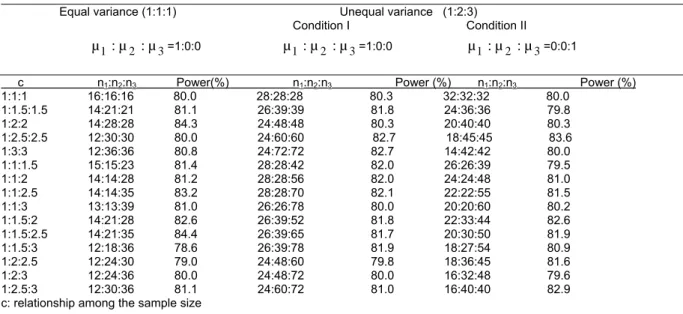
Table 1. Determining optimum sample size based on variance ratio and mean difference, k=3 Equal variance (1:1:1) Unequal variance (1:2:3)
Condition I Condition II
µ
1:
µ
2:
µ
3=1:0:0µ
1:
µ
2:
µ
3=1:0:0µ
1:
µ
2:
µ
3=0:0:1c n1:n2:n3 Power(%) n1:n2:n3 Power (%) n1:n2:n3 Power (%)
1:1:1 16:16:16 80.0 28:28:28 80.3 32:32:32 80.0 1:1.5:1.5 14:21:21 81.1 26:39:39 81.8 24:36:36 79.8 1:2:2 14:28:28 84.3 24:48:48 80.3 20:40:40 80.3 1:2.5:2.5 12:30:30 80.0 24:60:60 82.7 18:45:45 83.6 1:3:3 12:36:36 80.8 24:72:72 82.7 14:42:42 80.0 1:1:1.5 15:15:23 81.4 28:28:42 82.0 26:26:39 79.5 1:1:2 14:14:28 81.2 28:28:56 82.0 24:24:48 81.0 1:1:2.5 14:14:35 83.2 28:28:70 82.1 22:22:55 81.5 1:1:3 13:13:39 81.0 26:26:78 80.0 20:20:60 80.2 1:1.5:2 14:21:28 82.6 26:39:52 81.8 22:33:44 82.6 1:1.5:2.5 14:21:35 84.4 26:39:65 81.7 20:30:50 81.9 1:1.5:3 12:18:36 78.6 26:39:78 81.9 18:27:54 80.9 1:2:2.5 12:24:30 79.0 24:48:60 79.8 18:36:45 81.6 1:2:3 12:24:36 80.0 24:48:72 80.0 16:32:48 79.6 1:2.5:3 12:30:36 81.1 24:60:72 81.0 16:40:40 82.9 c: relationship among the sample size
Table 2. Determining optimum sample size based on variance ratio and mean difference, k=4
Equal variance (1:1:1:1) Unequal variance (1:2:3:4) Condition I Condition II
µ
1:
µ
2:
µ
3:
µ
4=1:0:0:0µ
1:
µ
2:
µ
3:
µ
4=1:0:0:0µ
1:
µ
2:
µ
3:
µ
4=0:0:0:1c n1:n2:n3:n4 Power(%) n1:n2:n3:n4 (max) Power (%) n1:n2:n3:n4 (min) Power (%)
1:1:1:1 16:16:16:16 81.1 34:34:34:34 81.7 42:42:42:42 80.0 1:1:1.5:1.5 16:16:24:24 83.9 34:34:51:51 81.6 32:32:48:48 80.0 1:1:2:2 14:14:28:28 80.3 34:34:68:68 81.5 26:26:52:52 80.0 1:1:2.5:2.5 14:14:35:35 82.0 34:34:85:85 82.2 24:24:60:60 81.9 1:1:3:3 14:14:42:42 83.0 34:34:102:102 82.5 20:20:60:60 79.8 1:1.5:2:2.5 14:21:28:35 82.3 32:48:64:80 80.8 22:33:44:55 80.0 1:1.5:2:3 14:21:28:42 83.4 34:51:68:102 82.9 20:30:40:60 79.8 1:2:2:3 14:28:28:42 83.6 32:64:64:96 81.7 20:40:40:60 82.9 1:2:2.5:3 14:28:35:42 83.5 32:64:80:96 82.5 20:40:50:60 83.5 1:1.5:2.5:3 14:21:35:42 83.9 32:48:80:96 80.0 20:30:50:60 81.1 1:1.5:1.5:3 14:21:21:42 82.4 34:51:51:102 82.6 22:33:33:66 82.2 1:2:2:3 14:28:42:42 84.0 32:64:96:96 82.6 18:36:54:54 79.5 References
Adcock, C. J. 1997. Sample Size Determination. The Statistician 46 (2): 261-283.
Alexander, R. A. and D. M. Govern. 1994. A new and simple approximation for ANOVA under variance heterogeneity. Journal of education Statistics 19: 91-101.
Algina, R. A., T. C. Oshima and W. Y. Lin. 1994. Type I error rates for Welch’s test and James’s second-order test under nonnormality and inequality of variance when there are two groups. Journal of Educational and Behavioral Statistics 19: 275-291.
Anonymous, 1994. FORTRAN subroutines for Mathematical Applications. IMSL MATH/LIBRARY. Vol.1-2. Visual Numerics, Inc., Houston, USA.
228 TARIM BİLİMLERİ DERGİSİ 2005, Cilt 11, Sayı 3
Bratcher, T. L., M. A. Moran and W. J. Zimmer. 1970. Tables of sample sizes in the analysis of variance. Journal of Quality Technology 15: 33-39.
Box, G. E. P. 1954. Some theorems on quadratic forms applied in the study of analysis variance problems, I. effect of inequatiley of variance in the one-way model. The Annals of Mathematical Statistics 25: 290-302.
Brown, M. B. and A. B. Forsythe. 1974. The small sample behaviour of some statistics which test the equality of several means. Technometrics 16: 129-132.
Cohen, J. 1969. Statistical power analysis for behavioral science. New York: Academic Press.
Cohen, J. 1988. Statistical power analysis for the behavioral sciences. Second Ed. New Jersey: Lawrence Erlbaum Associates, Hillsdale.
Cook, C. M. A. and S. D. Raj. 2003. Making the concepts of power and sample size relevant and accessible to students in introductory statistics courses using applets. Journal of Statistics Education.
Desu, M. M. and D. Raghavarao. 1990. Sample size methodology. Boston: Academic Press.
Dupont, W. D. and W. D. Jr. Plummer. 1990. Power and sample size calculations: A review and computer program. Controlled Clinical Trials 11: 116-128.
Dupont, W. D. and W. D. Jr. Plummer. 1998. Power and sample size calculations for studies involving linear regression. Controlled Clinical Trials 19: 589-601.
Eckblad, J. W. 1991. How many samples should be taken? BioScience 41 (5): 346-348.
Elliott, J. M. 1977. Some methods for the statistical analysis of samples of benthic invertebrates. 2nd Edition. Freshwater Biological Association Scientific Publication No. 25. Fenstad, G. U. 1983. A comparison between U and V tests in the
behrens-fisher problem. Biometrika 70: 300-302.
Ferron J. and C. Sentovich. 2002. Statistical power of randomization tests used with multiple- baseline designs. Journal of Experimental Education 70 (2): 165-178. Gatti, G. G. and M.Harwell, 1998. Advantages of computer
programs over power charts for the estimation of power. Journal of Statistics Education,6(3).
Glass, G. V., P. D. Peckham and Jr. Sanders. 1972. Consequences of failure to meet assumptions underlying analysis of variance and covariance. Review of Educational Research 42: 237-288.
Hicks, C. R. 1993. Fundamental Concepts in the Design of Experiments (4th ed.) New York: Saunders College Publishing.
Hoening, J. M. and D. M. Heisey. 2001. The abuse of power: The prevasive fallacy of power calculations for data analysis. The American Statistician 55: 19-24.
Horn, M. and R. Vollandt. 1998. Sample sizes for comparisons of k treatments with a control based on different definitions of power. Biometrical Journal 40: 589-612.
Horn, M., R. Vollandt and C. W. Dunnett. 2000. Sample size determination for testing whether an identified treatment is best. Biometrics 56: 70-72.
Lenth, R. V. 2001. Some practical guidelines for effective sample size determination. The American Statistician 55: 187-193. Mendeş, M. 1998. Sample size determination in parameter
estimation and testing of hypothesis for between difference among k-group means. MsD. Thesis. Thesis. Ankara University Graduates School of Natural and Applied Sciences Department of Animal Science (unpublished). Mendes, M. 2002. The comparison of some parametric alternative
test to one-way analysis of variance in terms of Type I error rates and power of test under non-normality and heterogeneity of variance. Ph.D. Thesis. Ankara University Graduates School of Natural and Applied Sciences Department of Animal Science (unpublished).
Mendes, M. and A. Pala. 2004. Evaluation of four tests when normality and homogeneity of variance assumptions are violated. Pakistan Journal of Information and Technology 4 (1): 38-42.
Mendes, M. and B. Tekindal. 2002. Normal ve normal olmayan populasyonlarda ortalamalar arası farkın testinde uygun örnek genişliğinin belirlenmesi. Gazi Üniversitesi Endüstriyel Sanatlar Eğitim Dergisi 11: 25-38.
Montgomery, D. C. 2001. Design and Analysis of Experiments (5th
ed.) John Wiley and Sons. New York.
Nelson, L. S. 1985. Sample size tables for analysis of variance. Journal of Quality Technology 17 (3): 167-169.
Ott, L. 1998. An introduction to statistical methods and data analysis. Third Edition. PWS-Kent Publishing Company. Schneider, P. J. and D. A. Penfield. 1997. Alexander and
Govern’s approximation: Providing an alternative to ANOVA under variance heterogeneity. The Journal of Experimental Education 65: 271-286.
Vollandt, R., M. Horn and P. K. Sen. 2000. Sample size determination of Steel’s nonparametric many-one test. Commun.Statist.-Theory Meth. 29: 2915-2919.
Wilcox, R. R., V. L. Charlin and K. L. Thompson. 1986. New monte carlo results on the robustness of the ANOVA F, W and F* statistics. Journal of Statistical Computation and
Simulation 15: 33-943.
Wilcox, R. R. 1988. A new alternarive to the ANOVA F and new results on James’s second-order method. British Journal of Mathematical and Statistical Psychology 41: 109-117. Winer,B. J., D. R. Brown and K. M. Michels. 1991. Statistical
principles in experimental design. New York: McGraw-Hill Book Company.
Zar, J. H. 1999. Biostatistical analysis. New Jersey: Prentice –Hall Inc. Simon and Schuster/A Viacom Company.
İletişim adresi: Mehmet MENDEŞ
Çanakkale Onsekiz Mart Üniv. Ziraat Fak. Zootekni Bölümü-Çanakkale