The Comparison of Robust Partial Least Squares Regression Methods (RSIMPLS, PRM) with Robust Principal Component Regression for Predicting Tourist Arrivals to Turkey

(1)

Doğuş Üniversitesi Dergisi, 20 (1) 2019, 31-47

(1)_{Hacettepe Üniversitesi, İstatistik Bölümü, espolat@hacettepe.edu.tr} Geliş/Received: 02-10-2017, Kabul/Accepted: 24-12-2018

The Comparison of Robust Partial Least Squares Regression

Methods (RSIMPLS, PRM) with Robust Principal Component

Regression for Predicting Tourist Arrivals to Turkey

Türkiye’ye Gelen Yabancı Turist Sayısını Kestirmek için Sağlam Kısmi En Küçük Kareler Regresyon Yöntemlerinin (RSIMPLS, PRM) Sağlam Temel Bileşenler

Regresyon Yöntemi ile Karşılaştırılması

Esra POLAT (1)

ABSTRACT: Tourism is one of the most important component in the economic development strategy of many developing countries such as Turkey. The annual data set of Turkey (1986 - 2013), including the six factors affecting the tourist arrivals, is examined. The aim of this study is modelling the tourist arrivals to Turkey in cases of both multicollinearity and outlier existence in the data set by using a robust Principal Component Regression method: RPCR, two robust Partial Least Squares Regression methods: RSIMPLS and Partial Robust M-Regression (PRM). Hence, the best model giving the best predictions of tourist arrivals is selected and the most important factors are determined.

Keywords: multicollinearity, outliers, robust principal component regression, robust partial least squares regression, tourist arrivals

Jel Classification Code: C52

ÖZ: Turizm, Türkiye gibi gelişmekte olan ülkelerin ekonomik kalkınma stratejilerinde anahtar bileşendir. Türkiye’nin 1986 - 2013 dönemi için, gelen yabancı turist sayısını etkileyen altı faktörün dâhil olduğu veri kümesi incelenir. Bu çalışmanın amacı, veri kümesinde hem çoklu bağlantı hem de uç değer olduğunda Türkiye’ye gelen yabancı turist sayısını bir sağlam Temel Bileşenler Regresyon yöntemi: RPCR, iki sağlam Kısmi En Küçük Kareler Regresyon yöntemleri: RSIMPLS ve Kısmi Sağlam M-Regresyon (PRM) kullanarak modellemektir. Böylece, yabancı turist sayısının en iyi kestirimlerini veren en iyi model seçilir ve en önemli faktörler belirlenir.

Anahtar Kelimeler: çoklu bağlantı, aykırı değerler, sağlam temel bileşenler

regresyonu, sağlam kısmi en küçük kareler regresyonu, gelen turist sayısı

1. Introduction

In existence of multicollinearity in the data set, Multiple Linear regression (MLR) analysis gives unreliable estimates for regression parameters and the variance of these parameters could be too large that leads to use biased methods: Principal Component Regression (PCR) and Partial Least Squares Regression (PLSR). Since they firstly reduce the dimensionality of the design matrix, they are the most popular regression techniques yielding better solutions. Straightforward Implementation of a Statistically Inspired Modification of the Partial Least Squares Method (SIMPLS) algorithm is the most popular PLSR algorithm as it is fast, efficient and the results of it are easily

(2)

32 Esra POLAT

interpreted. Since PCR is a combination of Principal Component Analysis (PCA) on the x-variables with Least Squares (LS) regression, in the case of outliers existence both steps of it are unreliable. Moreover, also the results of SIMPLS are affected by outliers in the data set as it is based on the empirical cross-covariance matrix between the y-variables and the x-variables and on linear LS regression. Hence, in Hubert and Verboven (2003) and Hubert and Vanden Branden (2003), two robust versions of these methods: RPCR and RSIMPLS have been suggested respectively. Another robust PLSR method ‘Partial Robust M-Regression (PRM)’ is conceptually different: instead of robust Partial Least Squares (PLS), Serneels et al. (2005) proposed a partial robust regression estimator.

World Travel & Tourism Council (WTTC) state clearly that both of travel and tourism are the top industries in the world on almost any economic measure, including gross output, value added, capital investment, employment and tax contributions (Aslan et al., 2008). Turkey and many developing countries utilize tourism as a key component in their economic development strategy. Turkey is a developing country which is both a candidate country for European Union membership and one of the attractive touristic places in the south of Europe. Since it contributes to Gross Domestic Product, tourism is one of the prominent industries in the Turkish economy. Since particularly from 1980’s Turkey’s active outer tourism started to show important development, tourism which contributes to the country’s economy results in a very huge source of income. In 1982, forming of mass tourism investment is started. The bill on incentives for tourism introduced in 1982 (Tourism Intensive Law No. 2634) contributed to the development of the sector and the tourism actors included in tourism activities. This law caused rapidly increment in tourism investments and increase the foreign number of tourists coming to Turkey and as a result the income of tourism increased within the share of Gross National Product. It seems that the number of foreign visitors has accelerated rapidly in last decade. In 2004, Turkey attracted 17.5 million foreign tourists, exceeding 41 million visitors in 2014.

There are many and various modelling and forecasting techniques for tourist arrivals. There isn’t only one special model that exactly performs better than the other models in every situation. One of the forecasting method in tourism is predicting foreign tourist arrivals to particular countries. Different methods have been used in determining the determinants of demand for international tourism. It is clear that multiple regressions were used mostly in tourism demand researches. Approximately

in 84% of tourism demand studies seemed to have used MLR (Zhang, et al., 2009).

The aim of this study is to model the tourist arrivals (number of foreign tourists) to Turkey by using three popular biased robust RPCR, RSIMPLS and PRM methods in existence of both multicollinearity and outlier in the data set. Therefore, the best model giving the best predictions of tourist arrivals is selected and the most important factors affecting the tourist arrivals to Turkey are determined for the examined period.

2. Robust Biased Estimation Methods: Rpcr, Rsimpls, Prm

PCR and PLSR methods assume that the p-dimensional independent x-variables and a set of q-dimensional dependent y-variables are associated by using a bilinear model. n is the number of observations and for i=1,…,n this bilinear model is shown as in (1) and (2). Here ~t_i are scores with the dimension of k<<p, Pp,k is the x-loadings matrix

(3)

The Comparison of Robust Partial Least Squares Regression Methods (RSIMPLS, PRM) with Robust Principal Component Regression for Predicting Tourist Arrivals to Turkey

33

and Ak,q is the slope matrix for the regression model of yi on ~t_i. fi and gi are error terms. This bilinear model could be written in terms of the original independent variables as in (3). PCR and PLSR construct the scores ~t_i in a different way. PCR and PLSR differentiate mainly in the construction of the scores ~t_i. PCR method computes the scores by extracting the most related information in the x-variables by using a variance criterion (as a result of PCA on the independent variables). However, the PLSR scores are computed by maximizing a covariance criterion between the x- and y-variables (Hubert and Verboven, 2003; Hubert and Vanden Branden, 2003; Engelen et al., 2004). i p,k i i x  x P t g (1) i q,k i i

y

 

y A



t



f

(2) i 0 q ,p i i y   B x e (3) Hubert and Verboven (2003) and Hubert and Vanden Branden (2003) have suggested two robust types of these methods: RPCR and RSIMPLS, respectively. Another robust PLSR method called PRM is proposed by Serneels et al. (2005). In PRM method, weights ranging between zero and one are computed iteratively in order to reduce the influence of outliers both in the y and x spaces. PRM is very efficient in terms of computational cost and statistical properties (Serneels et al., 2005; Liebmann et al., 2010; Polat and Turkan, 2016).

2.1. Robust Principal Component Regression: RPCR

Before starting the PCR analysis, the data is centered as ~x_i x_ix and

y

_i



y

_i



y

. Afterwards, a PCA on the x-variables is performed in order to remove the effect of multicollinearity. The first k dominant eigenvectors of the covariance matrix

p , n n , p x X ~ X~ 1 n 1 S  

 is contained in PCA loading matrix ~P_k_,_p 



p₁,,p_k



 and the scores satisfy ~t_i P~_k_,_p~x_i. In the second step of PCR, the response variables ~ are y_i regressed onto ~t_i as ~y_i A~t_i ~_i using MLR. Then, the parameter estimates and fitted values are obtained as Aˆ_k_,_q 

 

TT _k_,1_kT_k_,_nY~_n_,_q and yˆ_i Aˆ_q_,_k~t_i y, respectively. The unknown regression parameters in model (3) are then estimated as

q , k k , p q , p P Aˆ ~

Bˆ  and ˆ₀ yBˆ_q_,_px (Hubert and Verboven, 2003).

Both steps of PCR is robustified and a robust PCR method is proposed by Hubert and Verboven (2003). In the first step, the highly robust Minimum Covariance Determinant (MCD) estimator is used as a robust estimator of the covariance matrix of the xi in case of the data has a low-dimension (p<n/2), however, in case high-dimensional data the ROBPCA method chosen. ROBPCA, which combines projection pursuit ideas with MCD covariance estimation in lower dimensions, is a robust PCA method. In MCD estimator, the subsets of size h out of the whole data set

(4)

34 Esra POLAT

(of size n) is examined. Later the MCD estimator searches to find h subset for whom classical covariance matrix has minimal determinant. The robustness of the estimator is determined by the number ‘h’ that must be at least (n+p+1)/2. The MCD location estimate shown by x_h and the MCD scatter estimator shown by its covarince matrix

h

ˆ

 . A tolerance ellipse, capturing the covariance structure of the majority of the data points, is yielded by a robust PCA method. The highly robust MCD estimator of location and scatter (ˆ_MCD and ˆ_MCD) applied to the data and the points x of whose robust distance D

 

x D



x,ˆ_MCD,ˆ_MCD







xˆ_MCD



ˆ_MCD1



xˆ_MCD



equals to

2 975 . 0 , 2

 are plotted for the purpose of yielding a robust tolerance ellipse. In order to increase finite sample efficiency substantially, the raw MCD estimate can be reweighted. So that each data point belonging to the robust tolerance ellipse takes a weight of one and in other case a weight of zero. Therefore, the classical mean and covariance matrix of the data points having weight one gives reweighted MCD estimator. At last, robust loadings are obtained by the first k eigenvectors of the MCD estimator that ranked in descending order of the eigenvalues (Hubert and Verboven, 2003; Engelen et al., 2004).

In the second step of RPCR method, if there is only one y-variable the reweighted Least Trimmed Squares (LTS) regression is chosen for regressing y on i t , otherwise i the MCD regression is applied. Here, the regression model with intercept written as in (4) with _Cov

 

 __{. In case of one response variable (q=1), this model simplifies} as in (5) with __{scale of the errors. The parameters in (5) could be estimated by} using the LTS estimator. The raw LTS estimator minimizes the sum of the h smallest squared residuals as shown in (6). Here, r_1:n2 r_2:n2  r_n:n2 denote the ranked squared residuals. A starting estimate of the error dispersion is shown in (7). Here c h is a consistency factor for normally distributed errors. Hence, the LS estimator performed on the observations whose absolute standardized residual is not too large corresponding to the reweighted LTS estimator. That means, if



ˆ,ˆ



/ˆ 2.5

ri  0 LTS 0  it is set wi 0 and otherwise, wi 1. Then, final estimates of



 

ˆ ˆ

,

0



are computed as the vector minimizing







     n 1 i 2 0 i i i y t w . i 0 i i

y

  

A t



 

(4) i 0 i

y

     



t

(5)









0 h 2 0 LTS 0 , i 1 i:n

ˆ ˆ

,

arg min

r

,

  

 





 

(6)









h 2 0 h 0 LTS i:n i 1

1 ˆ ˆ

ˆ

c

r

,

h



 



 

(7)

(5)

35

In case of q>1, the MCD regression estimator is used. First of all, the reweighted MCD estimator is calculated on the



t_i,y_i



jointly, hence, (k+q)-dimensional location estimate ˆ 



ˆ_t,ˆ_y



and a scatter estimate ˆ_k__q_,_k__q are obtained as shown in (8). Secondly, similar to the MLR estimates, which are based on the emprical covariance matrix of the joint



t_i,y_i



variables, robust parameter estimates are estimated as shown in (9). A reweighting step is done for increasing the efficiency of this robust regression estimator’s efficiency. To apply this reweighting scheme, each data point receives a zero weight if it is initial residual distance is unsually large as shown in (10), with (11) and (12). All other observations have a weight w_i 1. Later, the reweighted MCD regression parameters related to the MLR estimates based on observations having weight one. Updating the reweighted estimates for A and ˆ0 in (9), (11) and (12), the final residual distances are obtained. A different notation for the final estimates and residual distances is not used. The fitted values are obtained as in (13) and regression parameters derived as in (14). Finally, ˆ_ˆ__{is set (Hubert} and Verboven, 2003) t ty MCD yt y

ˆ



















(8) 1 k,q t ty

ˆ

ˆ ˆ

A

  

     ˆ₀ ˆ_y Aˆˆ_t

    

ˆ

_

ˆ

_y

A

ˆ



ˆ

_t

A

ˆ

(9) i

w



0

if

RD

_i

 

2_{q ,0.975} (10) i i ˆ i ˆ0 r y A t   (11)





1 i i

ˆ

i

ˆ

i

RD



D r , 0,

 

_

r





_

r

(12)





i q ,k i 0 q ,k k ,p i x 0

ˆ

_ˆ

ˆy

A

t

ˆ

_ˆ

A

P

x





 

 



   

(13) p,q p,k k ,q

ˆ

ˆB



P A

   

ˆ

₀

ˆ

₀

B

ˆ

_p,q



ˆ

_x (14) 2.2. Robust Partial Least Squares Regression: RSIMPLS

SIMPLS algorithm assuming that the x and y variables are related through a bilinear model as given in (1) and (2). After mean centering the data as X~





x_i x





_in_₁ and









n 1 i i y y

Y~  _ , firstly, SIMPLS will obtain k latent variables (LVs)





  _,_k ₁ _n n t ~ , , t ~ T ~

 and after the response variables will be regressed on these k LVs. K components (the columns of Tn,k

~

), which have maximum covariance with a certain linear combination of the y-variables, are constructed as a linear combination of the x-variables. In order to obtain k components, firstly, it is needed to calculate weight vectors. The first normalized PLSR weight vectors r1 and q1 are obtained as the first

(6)

36 Esra POLAT

left and right singular eigenvectors of S_yx S_xyX~_p_,_nY~_n_,_q /



n1



. The first coordinate of the score ~t_i is computed as ~t_i₁~x_ir₁ for each observation. If we need

that t t 0 n 1 i ib ia 





and ab (that means orthogonality of components), other PLSR weight vectors are computed by deflating the Sxy matrix. Firstly, computing the x-loading pjSxrj/



rjSxrj



with Sx then this deflation is made. Later p1,…,pa is orthonormalised as 1,…,a and the deflation of Sxy is made as



a 1



xy a a 1 a xy a xy S S

S      with S1_xy S_xy. Then, ~ ’s are defined as t_i ~t_ia ~x_ir_a or similarly as matrix form T~_n_,_k X~_n_,_pR_p_,_k with R_p_,_k 



r₁,,r_k



. Lastly, regressing the response variables yi on these k-dimensional scores ~t_i by using MLR, the formal regression model is obtained as in (15). Here, E

 

fi 0 and Cov

 

fi f . MLR yields estimates as in (16), (17) and (18). By inserting ~t_i R_k_,_p



x_ix



in (2), the parameters’ estimators of the original model are obtained as in (19) (Hubert and Vanden Branden, 2003; Engelen et al., 2004; Polat and Turkan, 2016).

i 0 q ,k i i y   A t f (15)

 

1





1 k ,q t ty k ,p x p,k k ,p xy ˆA  S  S  R S R  R S (16) 0

ˆ

q ,k

ˆ

y

A



t

  

(17) f y ˆq,k tˆk,q q,n n,q ˆq,k k,n n,kˆk,q S S A S A Y Y A T T A  (18) p,q p,k

ˆ

k ,q

ˆB



R

A

and

  

ˆ

₀

y

B x

ˆ



_{q ,p} (19) A robust RSIMPLS method starts by applying ROBPCA on the x- and y-variables with the aim of replacing Sxy and Sx, which are used in computing ~t_i, by robust counterparts and then continues similar to the SIMPLS algorithm. Similar to RPCR instead of MLR a robust regression method (ROBPCA regression) is performed in the second stage (Hubert and Vanden Branden, 2003; Engelen et al., 2004). To obtain robust scores, firstly, ROBPCA is applied on Z_n_,_m 



X_n_,_p,Y_n_,_q



. ROBPCA is robust covariance estimator for high-dimensional data sets (m>n). The outlyingness of every observation is calculated and later the empirical covariance matrix of the h observations with smallest outlyingness is considered by ROBPCA using projection pursuit ideas. The data are then projected onto the subspace K spanned by the ₀

m

k₀  dominant eigenvectors of this covariance matrix. Later the MCD method is applied to estimate the center and scatter of the data in this low dimensional subspace. Finally, these estimates are back transformed to the original space and a robust estimate of the center ˆ_z of Z_n_,_m and of its scatter ˆ_z are computed. This scatter matrix can be decomposed as ˆ_zPzLz

 

Pz with robust Z-eigenvectors _mz_,_k

0 P and Z-eigenvalues





0 0,k k L

diag . Diagonal matrix Lz containing the k largest ₀ eigenvalues of ˆ_z in decreasing order. Then Z-scores Tz can be computed by

(7)

37





z

z n z _Z ₁ _ˆ _P

T    . After the application of ROBPCA on Z_n_,_m, this yields robust estimates ˆ_z



ˆ_x,ˆ_y



 and ˆ_z. ˆ_z can be decomposed as in (20). The cross-covariance matrix _xy is estimated by ˆ_xyand the PLS weight vectors ra are computed as in the SIMPLS algorithm, but now starting with ˆ_xy instead of S_xy. The x-loadings are defined as p_j 



r_jˆ_xr_j



1ˆ_xr_j. Then the deflation of the scatter matrix ˆa_xy is performed as in SIMPLS. In each step the robust scores are calculated as in (21), where the x_i are the robustly centered observations (Hubert and Vanden Branden, 2003). x xy z yx y

ˆ



 















(20)





ia i a i

ˆ

x a

t



x r





x

 



r

(21) After the robust scores are derived, a robust linear regression is performed. The regression model, based on robust scores, is written as in (22). In order to estimate parameters in this model a robust regression method called ROBPCA regression is used (Hubert and Vanden Branden, 2003).

i 0 q ,k i i

y

  

A t





f

(22) ) k ( i

r is the residual for the ith observation based on the initial estimates which were

computed with k components and ˆ_f is the initial estimate of the covariance matrix of the errors. The robust distance of the residuals is given as in (23). The weights c_i_{ }_k are computed as in (24). Here I shows the indicator function. Observations with weight

 k i

c equal to one are used to compute the final regression estimates (similar to MLR method). The robust residual distances RD_i_{ }_k are recalculated as in (23) and at the same time the weights c_i_{ }_k are updated. Finally, robust parameter estimators of the original model (3) are obtained as in (25).

 



   



1/ 2 1 i k i k

ˆ

f i k

RD



r







r

(23)  



2  q ,0.9752



i k i k

c



I RD

 

(24) 0 0 q ,p x

ˆ

_ˆ

_B

ˆ

_

_ˆ

   



ˆB

_p,q



R

_p,k

A

ˆ

_{k ,q} (25)

(8)

38 Esra POLAT

2.3. Partial Robust M-Regression (PRM)

The latent regression model is then given by (26). Here T is a score matrix of size

n



k

, having as rows the vectors

t

_i, with

1  

i

n

(Serneels et al., 2005):

i i i

y

   

t

(26) Here, the vector



_k_₁ can be estimated by regressing the response variable on the LVs (t_i) by means of a robust M-estimator. The new model dimension is lower than as k < p and it is a regression on the score vectors (t ) that must be determined. _i Generally, leverage points and vertical outliers could be effective while estimating the regression coefficients, PRM gives robust parameter estimations. In PRM, a weight

x i

w is used to reduce the effect of leverage points, while a weight wr_i is used for reducing the effect of vertical outliers.

w

_ir are calculated from the residuals

i i i

r



y

 

t

and

w

_ix are obtained from the scores

t

_i (not from independent variables). In order to protect estimates against both vertical outliers and leverage points, weights need to be taken as in (27) and the obtained estimator called as the “PRM estimator” (Serneels et al., 2005).

r x i i i

w



w w

(27) In order to compute the score matrix T, the following scheme is used. Loading vectors

,

h

a

for h1, , k are computed in a sequential manner as in (28), under the constraint in (29).

Cov

_W



y, u



, in (29), with u another vector of length n, shows a weighted covariance as in (30) (Serneels et al., 2005).





k W a

a



arg max Cov

y, X

(28)

a



1

and Cov_W



Xa, Xa_j



0 for 1 j k (29)

 

n W i i i i 1

1 Cov

y, u

w y u

n





(30) Since Ap×k is the matrix of loading vectors, the score matrix is obtained as

T



XA

. The final estimate for



can be obtained as

  

ˆ

A

ˆ

after the computation of



ˆ

(Serneels et al., 2005).

The weights in the above definitions are unknown and they are not fixed. First approximation of the estimator



ˆ

is computed by using an appropriate initial value for the weights. Then, the weights are recomputed using the preliminary parameter estimates and a second approximation of



ˆ

is obtained by again applying weighted PLS. After that the weights

w

_i are recomputed and the iteration process continues. Hence, the Iterative Reweighted Partial Least Squares (IRPLS) algorithm can be used

(9)

39

to compute



ˆ

. These continuous weights are iteratively executed for each observation, in order to minimise the negative influence of outliers in the regression model (Serneels et al., 2005).

2.3.1. PRM Algorithm

Since PRM can be calculated with a change in an algorithm proposed by Cummins and Andrews (1995) called as Iterative Reweighted Partial Least Squares (IRPLS) regression, the implementation of it is easy. PRM is entirely robust and also practical for high-dimensional data sets. It is significant to use robust initial values and relevant weights. The weights also have to depend on the scores for PRM, thus correcting for leverage points if presenting in the predictor space (Serneels et al., 2005; Liebmann et al., 2010).

The weights

w

_ir have been computed as in (31) with



ˆ

an estimate of residual scale and the function in (32) (Serneels et al, 2005).

r i i

r

w

f

, c

ˆ

















(31)

 

2

1 f z, c

z

1 c

















(32)

In (32) c is a tuning constant, used as c = 4. f is “Fair” weight function. Other weight functions could be used and Serneels et al. (2005) stated that it is not claimed any optimality properties for c=4. However, many numerical experiments revealed that the fair function used with c = 4 is a good compromise between robustness and statistical efficiency. If the tuning constant c increases to infinity, then the weight function becomes more and more flat, as a result, the PRM-estimator look likes more and more PLS (Serneels et al., 2005).

By using standardized residuals, the weights in (33) are calculated. A simple and robust choice for



ˆ

s the Median Absolute Deviation:



1 n



i j

i

j

ˆ

MAD r ,

, r

median r

 





. The weights

w

_ix measuring the

leverage of each score vector

t

_i are computed as in (33) (Serneels et al, 2005).

 

1 1 i L x i i i L

t

med

T

w

f

, c

median t

med

T























(33)

Here

.

used for the Euclidean norm and

 

1

L

med

T

shows the L1-median computed from the collection of score vectors



t ,

₁

, t

_n



; it is a robust estimator of

(10)

40 Esra POLAT

the center of k-dimensional score vectors. This

L

₁-median is a multivariate version of the sample median, also known as a spatial median and it could be computed very quickly. Coordinate-wise or component-wise median also could be used for estimating the multivariate median (Serneels et al, 2005).

The PRM steps could be given briefly as in the following (Serneels et al, 2005): 1. Robust starting values for the weights

w

_i



w w

r_i _ix are computed. The formula in (31) is used with r_i y_i median y_j _j for the residual weights and formula in (33) is used with the score vectors replaced by x for_i, 1 i n for the leverage weights. 2. PLSR analysis is performed by using SIMPLS algorithm on the (re)weighted data matrices

X

and

y

computed by multiplying each row of X and y with

w

_i . This PLS analysis results then in an update of



ˆ

and of the score matrix T. By dividing each row of T by

w

_i , score matrix T is updated.

3. The residuals

r

_i



y

_i

 

t

_i

ˆ

are recomputed and the weights

w

_i



w w

_ir x_i are updated using (31) and (33).

4. Go back to step (2) until



ˆ

converges. Whenever the relative difference in norm between two consecutive approximations of



ˆ

s is smaller than a specified threshold, e.g. 102, then convergence is achieved.

5. The final estimate



ˆ

is directly obtained from the last weighted PLS step. Many numerical computations revealed that this iterative procedure is stable and converges quite quickly. If software for computing standard PLS is available, then it is easy and quick to program the above algorithm (Serneels et al, 2005).

3. Application and Results

Tourism is one of the most quickly growing sectors in the world. Global tourism flows and tourism receipts show a stable increase in recent years. Hence, as an effective tool, significance of tourism on economic growth and development of a country increases. For most of the countries, tourism constitutes a prominent source of additional income, foreign exchange, employment and tax revenue. Turkey is one of the popular destinations in the world and today, tourism has become an important sector in the Turkish economy.

The tourism demand literature shows that there are several measurements for international tourism demand such as: the number of the tourist arrivals, the number of nights spent by tourist or the receipts from tourism. The number of tourist arrivals is still the most popular measurement in tourism demand studies. The main reason for this choice is the availability of tourist arrivals data. In this study, tourism demand is measured in terms of number of tourist arrivals to Turkey. Therefore, in order to develop the sector in a most planned and controlled manner it is important to determine the factors which have impact on Turkey’s tourist arrivals. In this paper, it

(11)

41

is aimed to investigate some of these effective factors based on robust biased methods since the data set contains both multicollinearity and outliers.

The purpose of this study is to model the tourist arrivals (number of foreign tourists) to Turkey for the period of 1986-2013 by using three popular biased robust RPCR, RSIMPLS and PRM methods in existence of both multicollinearity and outliers in the data set. The model giving the best predictions of tourist arrivals is selected and the most effective variables on the tourist arrivals to Turkey are found. Considering the studies of Alpu et al. (2010), Samkar et al. (2011) and Ispir et al. (2015) six independent variables are determined and a trend variable is also added to analysis. The variables in the models are given in below:

Y: Number of Foreign Tourists, T: Trend

X1: Number of Incoming Airplanes,

X2: Number of Rooms in Tourism Facilities, X3: Number of Rest Areas,

X4: Number of Licensed Operation Yachts, X5: Total Bed Amount of Tourism Facilities, X6: Number of Tourism Agencies,

Firstly, classical MLR model is applied and found to be significant with a probability of 95% (F=396.95; p=0.000). According the MLR analysis, 99.3% of variation occurs in the variable of number of foreign tourists is explained by these six independent variables. Even though the MLR model fits the data well, multicollinearity may severely prohibit quality of the prediction. Table 1 shows that all independent variables with the exception of X1 and X3 are not significant as an indicator of multicollinearity problem. Firstly, it is investigated whether there is multicollinearity or not in the dataset. For this purpose, the condition number is calculated as

max/min=7.240/0.006=1206.6. The condition number greater than 30 means that there is multicollinearity. The other multicollinearity measure is Variance Inflation Factor (VIF) that is one of the most common techniques in statistics for detecting multicollinearity. In practice, if any of the VIF values is equal or larger than 10, there is a near collinearity. In this case, the regression coefficients are not reliable. As the results of MLR the VIF values for T, X1, X2, X5 and X6 are found as 234.950, 15.450, 5314.895, 5129.155 and 68.604. Hence, there is a near-collinearity problem for this dataset.

(12)

42 Esra POLAT

Table 1. The estimated regression coefficients for the MLR model. Model Coefficients Standart Error

of Coefficients T P Constant 96832 1471796 0.66 0.518 T -237803 351877 -0.68 0.507 X1 58.32 15.11 3.86 0.001 X2 150.7 142.1 1.06 0.302 X3 -9193 1052 -8.74 0.000 X4 3217 1849 1.74 0.097 X5 -5.19 64.54 -0.08 0.937 X6 -342.9 748.8 -0.46 0.652

Secondly, whether outliers exist or not is examined using normal Q-Q plot of the MLR residuals given in Figure 1. As seen from Figure 1, there is an outlier in the data.

Figure 1. Normal Q-Q plot of MLR residuals

Table 1 shows that the significant variable X3 (Number of Rest Areas) has a negative effect on “Number of Foreign Tourists” variable which conflicts with both theoretical and logical expectations. Since the presence of both multicollinearity and outlier, the MLR results could not be reliable. In order to overcome both multicollinearity and outlier, biased robust RPCR and RSIMPLS, PRM methods (the robust counterparts of classical biased PCR and PLSR methods) are applied on the data set by using the functions given in MATLAB Toolboxes of ‘LIBRA Toolbox’ (Verboven and Hubert, 2005) and ‘TOMCAT Toolbox’ (Daszykowski et al., 2007).

(13)

43

The performance of the methods are evaluated by using the Root Mean Square Error

(RMSE),





n 2 i i i 1

ˆ

y

RMSE

n









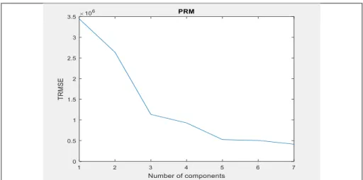
with upper % 20 trimming (TRMSE (0.8)), which is considered to be safer in the presence of outliers. Since we attend to assess the robust model’s performance in fitting the data but not the outliers, a robust RMSE measure is necessary. The exclusion of a certain percentage of unusually large (absolute) residuals leads to an acceptable robust performance criterion. As mentioned in Daszykowski et al. (2007), the obtained values of RMSE are trimmed according to the assumed fraction of data contamination.

Firstly, the optimal number of components (showed by kopt) could be selected for robust RPCR and robust PLSR methods (RSIMPLS and PRM) by taking the value for which TRMSE value is sufficiently small.

(14)

44 Esra POLAT

Figure 2. The plots of TRMSE (0.80) values of tourist arrival data set for RPCR, RSIMPLS, PRM

Since the model having sufficiently small TRMSE (0.80) value is always preferred, as seen from Figure 2 both of the RPCR and RSIMPLS models with two components (kopt=2) and PRM model with three components (kopt=3) is chosen.

Table 2. TRMSE values of three models for the tourist arrival dataset RPCR (kopt=2) RSIMPLS (kopt=2) PRM (kopt=3)

TRMSE (0.8) 8.5582e+05 8.9937e+05 1.1348e+06 As seen from Table 2, RPCR is the model giving the best prediction of number of foreign tourists, hence, the estimated coefficients for RPCR given as shown in below. The final model of RPCR is presented in terms of original variables:

Number of Foreign Tourists = -2.0969e+07 + 0.0037 trend + 40.1142 airplanes + 17.4722 rooms + 0.0407 restareas – 0.0175 yachts + 40.0919 bedamount + 1.0286 agencies

For the best model selected (RPCR) it is possible to detect outliers by using regression diagnostic plot and score diagnostic plot as shown in Figure 3. The first plot allows us to distinguish three types of outliers; good leverage points, bad leverage points and vertical outliers. The second one detects three types of outliers; good PCA leverage points, bad PCA leverage points and orthogonal outliers. The orthogonal outliers do not influence the computation of the regression parameters, but they might influence the loadings.

(15)

45

Figure 3. (a) Regression diagnostic plot (b) score diagnostic plot for RPCR (kopt=2)

Figure 3 gives the order numbers of the observations, which are outliers and detected by RPCR (kopt=2). It is seen that observations 1 and 2 are both vertical and orthogonal outliers, observations 3 and 4 are only vertical outliers, observations 27 and 28 are both good leverage and bad PCA leverage points.

4.Conclusion

The sector of tourism creates employment opportunities, decreasing unemployment and has an important role on providing the country with foreign currency income. Since it is a source of income and a supply of foreign currency input, it’s eliminating instability between regions, farming, transportation, services and other tourisms

(16)

46 Esra POLAT

concerning direct and indirect commercial activities gaining motion, tourism is very important for a country’s economy.

In this study, robust biased RPCR, RSIMPLS and PRM methods are applied to a real tourist arrival dataset of Turkey with both multicollinearity and outlier. They have been compared in order to determine which of them gives the best predictions of tourist arrivals. For the tourist arrival data set, RPCR model is chosen as the best model according to a robust RMSE performance criterion, TRMSE(0.8). The results obtained from RPCR robust biased estimation method showed that the most important independent variables affecting the number of foreign tourists are “Number of Incoming Airplanes” and “Total Bed Amount of Tourism Facilities”. The least important variables affecting the number of foreign tourists are “Number of Licensed Operation Yachts” and “Number of Rest Areas”. Hence, any increment in “Number of Incoming Airplanes” and “Total Bed Amount of Tourism Facilities” cause an important increment in number of foreign tourists. In this study, also it is observed that the addition or omission of the trend variable does not affect the results. Whether the trend variable present or not in the model, the parameters of independent variables remained same.

In conclusion, it could be declared that for the chosen best model RPCR, the directions of relationships between these six independent variables and the number of foreign tourists are consistent with the results obtained by Alpu et al. (2010), Samkar et al. (2011) and Ispir et al. (2015). Studies and meet the theoretical expectations. Moreover, in this study, different from other studies in literature about forecasting number of foreign tourists, three biased robust estimation methods RPCR, RSIMPLS and PRM are applied for the first time in the case of both multicollinearity and outlier existence.

5. References

Alpu, O., Samkar, H. and Altan, E. (2010). Saglam ridge regresyon analizi ve bir uygulama. Dokuz Eylul Universitesi İktisadi ve İdari Bilimler Fakultesi Dergisi, 25 (2), 137-148.

Aslan, A., Kaplan, M. and Kula, F. (2008). International tourism demand for Turkey: a dynamic panel data approach. Avaliable: https://mpra.ub.uni-muenchen.de/10601/1/MPRA_paper_10601.pdf.

Daszykowski, M., Serneels, S., Kaczmarek, K.., Van Espen, P., Croux, C. and Walczak, B. (2007). TOMCAT: A MATLAB toolbox for multivariate calibration techniques. Chemometrics and Intelligent Laboratory Systems, 85, 269–277. Engelen, S., Hubert, M., Vanden Branden, K. and Verboven, S. (2004). Robust PCR

and robust PLSR: a comparative study. M. Hubert, G. Pison, A. Struyf and S. V. Aelst (Ed.). In Theory and Applications of Recent Robust Methods (pp. 105–117). Birkhäuser; Basel.

Hubert, M. and Verboven, S. (2003). A robust PCR method for high-dimensional regressors. Journal of Chemometrics, 17, 438–452.

Hubert, M. and Vanden Branden, K. (2003). Robust methods for partial least squares regression. Journal of Chemometrics, 17, 537-549.

Ispir, D., Ergul, B. and Yavuz Altın, A. (2015). Examining the ridge regression analysis of the number of foreign tourists coming to Turkey, in Proceedings of the 2nd International Congress of Tourism & Management Researches (pp. 242).

(17)

47

Liebmann, B. Filzmoser, P. and Varmuza, K. (2010). Robust and classical PLS regression compared. Journal of Chemometrics, 24 (3-4), 111-120.

Polat, E. and Turkan, S. (2016). The comparison of classical and robust biased regression methods for determining unemployment rate in Turkey: period of 1985-2012. Journal of Data Science, 14 (4), 739-768.

Samkar, H., Alpu, O. and Altan, E. (2011). Ridge regresyonda M tahmin edicilerinin kullanımı üzerine bir uygulama. Dokuz Eylul Universitesi İktisadi ve İdari Bilimler Fakultesi Dergisi, 26 (1), 67-77.

Serneels, S., Croux, C., Filzmoser, P. and Van Espen, P. J. (2005). Partial robust M-regression. Chemometrics and Intelligent Laboratory Systems, 79, pp. 55-64. Verboven, S. and Hubert, M. (2005). LIBRA: a MATLAB library for robust analysis.

Chemometrics and Intelligent Laboratory System, 75, 127–136.

Zhang, Y., Qu, H. and Tavitiyaman, P. (2009). The determinants of the travel demand on international tourist arrivals to Thailand. Asia Pacific Journal of Tourism Research, 14 (1), 77-92.