Numerical simulation of optically trapped particles

PROCEEDINGS OF SPIE

SPIEDigitalLibrary.org/conference-proceedings-of-spie

Numerical simulation of optically

trapped particles

Giorgio Volpe

Giovanni Volpe

Numerical Simulation of Optically Trapped Particles

Giorgio Volpe

, Giovanni Volpe

a

_{Institut Langevin, ESPCI ParisTech, CNRS UMR7587, 1 rue Jussieu, 75005 Paris, France;}

_Physics

Department, Bilkent University, Cankaya, 06800 Ankara, Turkey

ABSTRACT

Some randomness is present in most phenomena, ranging from biomolecules and nanodevices to financial markets and human organizations. However, it is not easy to gain an intuitive understanding of such stochastic phenomena, because their modeling requires advanced mathematical tools, such as sigma algebras, the Itô formula and martingales. Here, we discuss a simple finite difference algorithm that can be used to gain understanding of such complex physical phenomena. In particular, we simulate the motion of an optically trapped particle that is typically used as a model system in statistical physics and has a wide range of applications in physics and biophysics, for example, to measure nanoscopic forces and torques.

Keywords: optical forces, Brownian motion, stochastic differential equations

1. INTRODUCTION

In this proceeding, we present a simple algorithm to simulate a Brownian particle in an optical trap [1]. We provide an implementation of this algorithm using MatLab®, because this language is widely employed in the science and engineering. All algorithms can also be translated straightforwardly in the freeware programming language SciLab [2]. The interest of these simulations is dual. On the one hand, it is interesting to simulate an optically trapped particle to gain insight into how an optical trap works; since optical traps have found a widespread set of applications in fields as diverse as, e.g., cooling of single atoms, colloidal physics and biophysics, it can be useful for many students to understand how these optical traps work in simple and inexpensive simulations. On the other hand, an optically trapped particle constitutes a simple example of a stochastic phenomenon whose evolution is determined by both stochastic (the Brownian motion) and deterministic (the optical forces) forcing terms and can, therefore, be used as a model system for more general stochastic phenomena.

2. LANGEVIN EQUATION

An optically trapped particle can be described by the Langevin equation in one dimension [1,3]:

m

d

dt

x(t) = −

γ

d

dt

x(t) − k

d

dt

x(t) + 2k

T

γ

W (t)

where x(t) is the trajectory of the particle with respect to the trap center, m is the particle mass, γ is the friction exerted by

the surrounding medium on the particle, k is the optical trap stiffness, kBT is the thermal energy unit, kB is the Boltzmann

constant, T is the absolute temperature and W(t) is a Wiener process.

For microscopic particles immersed in a liquid, viscous forces are several orders of magnitude larger than inertial forces, i.e. the particle is in a low-Reynolds-number regime [4]. The Reynolds number is the ratio between inertial and viscous forces acting on an object moving in a fluid. If the object has a characteristic dimension L and is moving at velocity v through a fluid with viscosity η and density ρ, its Reynold number is Re = Lvρ/η. In the low-Reynold-number regime, i.e for Re < 1, the viscosity dominates over inertia. Considering, for example, an E. coli bacterium in swimming in water [5], L ≈ 1µm, v ≈ 30µm/s, η = 0.001Pas and ρ = 1000kg/m3, so that Re = 3e-5 ≪ 1. One of the most striking aspect of low Reynolds number phenomena is that the speed of an object is solely determined by the forces acting on it at the

moment; a good introduction to how is life at low Reynold numbers can be found in Ref. [4]. In general, most optical manipulation experiments take place at low Reynolds numbers, the exceptions being experiments in fluids with very low viscosity such as air [6]. Therefore, in Eq. (1) we can drop the inertial term obtaining:

d

dt

x(t) = −

k

γ

d

dt

x(t) +

2k

T

D

W (t)

where D is the Stokes-Einstein diffusion coefficient.

Eq. (2) is one of the simplest examples of a stochastic differential equation [7,8]. In general, stochastic differential equations are obtained from ordinary differential equations adding a noise term, i.e. the Wiener process W(t). W(t) is characterized by the following properties:

1. the mean <W(t)> = 0 for all t; 2. <W(t)2_{> = 1 for each value t;}

3. W(t1) and W(t2) are independent of each other for t1 different from t2. Because of these properties, a white noise is not

a standard function. In particular, W(t) is almost everywhere discontinuous and has infinite variation. In an intuitive picture, it can be seen as the continuous-time equivalent of a discrete sequence of independent random numbers.

3. FINITE-DIFFERENCE SOLUTION

In order to simulate Eq. (2) it is possible to employ a finite difference algorithm, where the continuous-time solution x(t) is approximated by a discrete time sequence xi evaluated at times ti = i Δt. This is in practice done by doing the following

substitutions in Eq. (2) [1,7]: 1.

x(t)

→

x

d

dt

x(t)

→

x

− x

Δt

W (t)

→

w

Δt

where wi is a sequence of Gaussian random numbers with the following properties:

1. the mean <wi> = 0;

2. <wi2> = 1;

3. <wi wj > = 0 for i different from j.

Notice how these properties mimick the ones of the Wiener process given above.

By making the aforementioned substitutions in Eq. (2) one obtains the following finite difference equation:

x

= x

−

k

γ

x

Δt + 2DΔt w

which can now be solved numerically.

4. SIMULATION CODE

In this section we present the MatLab® code that implements Eq. (3) in one and 3 dimensions following the codes provided with Ref. [1].

4.1 1D Simulation Code

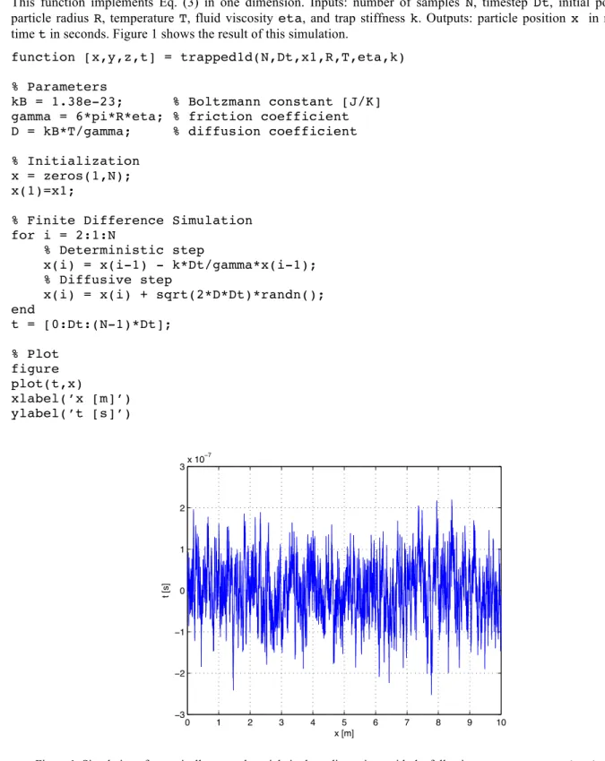
This function implements Eq. (3) in one dimension. Inputs: number of samples N, timestep Dt, initial position x1, particle radius R, temperature T, fluid viscosity eta, and trap stiffness k. Outputs: particle position x in meters and time t in seconds. Figure 1 shows the result of this simulation.

function [x,y,z,t] = trapped1d(N,Dt,x1,R,T,eta,k)

% Parameters

kB = 1.38e-23; % Boltzmann constant [J/K] gamma = 6*pi*R*eta; % friction coefficient D = kB*T/gamma; % diffusion coefficient

% Initialization x = zeros(1,N); x(1)=x1;

% Finite Difference Simulation for i = 2:1:N

% Deterministic step

x(i) = x(i-1) - k*Dt/gamma*x(i-1); % Diffusive step

x(i) = x(i) + sqrt(2*D*Dt)*randn(); end t = [0:Dt:(N-1)*Dt]; % Plot figure plot(t,x) xlabel(’x [m]’) ylabel(’t [s]’) 0 1 2 3 4 5 6 7 8 9 10 −3 −2 −1 0 1 2 3x 10 −7 x [m] t [s]

Figure 1. Simulation of an optically trapped particle in three dimensions with the following parameters: N = 1e+4; Dt = 1e-3 [s]; x1 = 0 [m]; R = 1e-6 [m]; T = 300 [K]; eta = 0.001 [Pa s – water]; kx = 1e-6 [N/m] [N/m].

4.2 3D Simulation Code

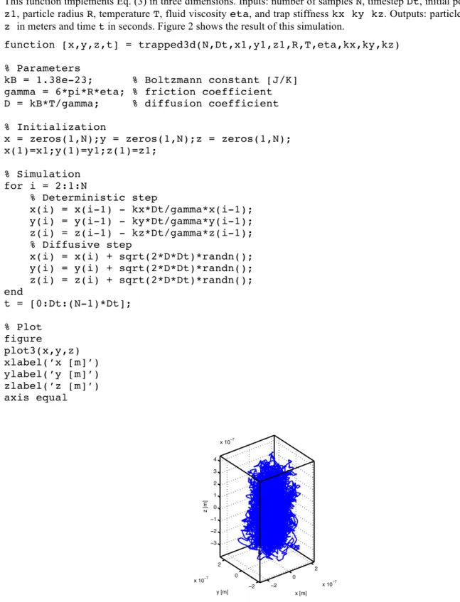
This function implements Eq. (3) in three dimensions. Inputs: number of samples N, timestep Dt, initial position x1 y1 z1, particle radius R, temperature T, fluid viscosity eta, and trap stiffness kx ky kz. Outputs: particle position x y z in meters and time t in seconds. Figure 2 shows the result of this simulation.

function [x,y,z,t] = trapped3d(N,Dt,x1,y1,z1,R,T,eta,kx,ky,kz)

% Parameters

kB = 1.38e-23; % Boltzmann constant [J/K] gamma = 6*pi*R*eta; % friction coefficient D = kB*T/gamma; % diffusion coefficient

% Initialization

x = zeros(1,N);y = zeros(1,N);z = zeros(1,N); x(1)=x1;y(1)=y1;z(1)=z1;

% Simulation for i = 2:1:N

% Deterministic step

x(i) = x(i-1) - kx*Dt/gamma*x(i-1); y(i) = y(i-1) - ky*Dt/gamma*y(i-1); z(i) = z(i-1) - kz*Dt/gamma*z(i-1); % Diffusive step

x(i) = x(i) + sqrt(2*D*Dt)*randn(); y(i) = y(i) + sqrt(2*D*Dt)*randn(); z(i) = z(i) + sqrt(2*D*Dt)*randn(); end t = [0:Dt:(N-1)*Dt]; % Plot figure plot3(x,y,z) xlabel(’x [m]’) ylabel(’y [m]’) zlabel(’z [m]’) axis equal −2 0 2 x 10−7 −2 0 2 x 10−7 −3 −2 −1 0 1 2 3 4 x 10−7 x [m] y [m] z [m]

Figure 2. Simulation of an optically trapped particle in three dimensions with the following parameters: N = 1e+4; Dt = 1e-3 [s]; x1 = 0 [m], y1 = 0 [m], z1 = 0 [m]; R = 1e-6 [m]; T = 300 [K]; eta = 0.001 [Pa s – water]; kx = 1e-6 [N/m], ky = 1e-6 [N/m], kz = 0.2e-6 [N/m].

5. DIFFUSION GRADIENTS

In the presence of diffusion gradients, which arise naturally, e.g., when a Brownian particle is trapped near another particle or near a surface, some additional correction are needed in order to account for a spurious drift [9,10,11,12]. This spurious drift results from the fact that the Wiener process is multiplied by a function of the particle position and is needed to correct an indetermination inherently occurring in stochastic differential equations with multiplicative noise. How to deal with these cases is explained in Refs. [13,14]. Similar considerations hold also in the case of diffusion gradients induced by, e.g., chemical gradients or temperature gradients [15,16,17].

6. FURTHER NUMERICAL EXPERIMENTS

Using the code provided in Section 4, it is possible to simulate an optically trapped particle under various conditions and verify, e.g., that the particle variance in the optical trap is inversely proportional to the trap stiffness [18]. Furthermore, it can be interesting to apply these simulation techniques to simulate and study the behavior of a Brownian particle in more complex force fields: for example, a Brownian particle in the presence of external forces or torques [19,20,21,22,23,24,25,26,27,28]. Also time-varying force fields can be considered, which leads to more complex phenomena, such as Kramers transitions [29], stochastic resonant damping [30] and stochastic resonance [31].

REFERENCES

[1] Volpe, G. and Volpe, G., “Simulation of a Brownian particle in an optical trap,” Am. J. Phys. 81, 224-230 (2013).

[2] Scilab < www.scilab.org/>.

[3] Nelson E., Dynamical Theories of Brownian Motion (Princeton University Press, Princeton, NJ, 1967). [4] Purcell, E. M., “Life at low Reynolds numbers,” Am. J. Phys. 45, 3-11 (1977).

[5] Berg, H., E. coli in Motion (Springer Verlag, New York, NY, 2004).

[6] Li, T., Kheifets, S., Medellin, D., Mark G. Raizen, M. G., “Measurement of the instantaneous velocity of a brownian particle,” Science 328, 1673-1675 (2010).

[7] Øksendal, B., Stochastic Differential Equations, 6th ed. (Springer, Heidel- berg, 2003).

[8] Kloeden, P. E., and Platen, E., Numerical Solution of Stochastic Differential Equations (Springer, Heidelberg, 1999).

[9] Ermak, D. L., and McCammon, J. A., “Brownian dynamics with hydrodynamic interactions,” J. Chem. Phys.

69, 1352-1361 (1978).

[10] Lançon, P., Batrouni, G., Lobry, L., and Ostrowsky, N., “Drift without flux: Brownian walker with a space-dependent diffusion coefficient,” Europhys. Lett. 54, 28 (2001).

[11] Lau, A. W. C., and Lubensky, T. C., “State-dependent diffusion: Thermodynamic consistency and its path integral formulation,” Phys. Rev. E 76, 011123 (2007).

[12] Hottovy, S., Volpe, G., and Wehr, J., “Noise-Induced Drift in Stochastic Differential Equations with Arbitrary Friction and Diffusion in the Smoluchowski-Kramers Limit,” J. Stat. Phys. 146, 762-773 (2012).

[13] Volpe, G., Helden, L., Brettschneider, T., Wehr, J., and Bechinger, C., “Influence of Noise on Force Measurements,” Phys. Rev. Lett. 104, 170602 (2010).

[14] Brettschneider, T., Volpe, G., Helden, L., Wehr, J., and Bechinger, C., “Force measurement in the presence of Brownian noise: Equilibrium-distribution method versus drift method,” Phys. Rev. E 83, 041113 (2011). [15] Hottovy, T., Volpe, G., and Wehr, J., “Thermophoresis of Brownian particles driven by coloured noise,” EPL

99, 60002 (2012).

[16] Ebbens, S. J., and Howse, J. R., “In pursuit of propulsion at the nanoscale,” Soft Matter 6, 726-738 (2010). [17] Howse, J. R., Jones, R. A. L., Ryan, A. J., Gough, T., Vafabakhsh, R., and Golestanian, R., “Self-motile

colloidal particles: from directed propulsion to random walk,” Phys. Rev. Lett. 99 048102 (2007).

[18] Volpe, G., Wehr, J., Rubi, J. M., and Petrov, D., “Thermal noise suppression: how much does it cost?” J. Phys. A: Math. Theor. 42 095005 (2009).

[19] Ashkin, A., “Optical trapping and manipulation of neutral particles using lasers,” Proc. Natl. Acad. Sci. U.S.A. 94, 4853-4860 (1997).

[20] Berg-Sorensen, K., and Flyvbjerg, H., “Power spectrum analysis for optical tweezers,” Rev. Sci. Instrum. 75, 594-612 (2004).

[21] Rohrbach, A., Tischer, C., Neumayer, D., Florin, E.-L., and Stelzer, E. H. K., “Trapping and tracking a local probe with a photonic force microscope,” Rev. Sci. Instrum. 75, 2197-2210 (2004).

[22] Bishop, A. I., Nieminen, T. A., Heckenberg, N. R., and Rubinsztein-Dunlop, H., “Optical application and measurement of torque on microparticles of isotropic nonabsorbing material,” Phys. Rev. A 68, 033802 (2003). [23] La Porta, A., and Wang, M. D., “Optical torque wrench: Angular trapping, rotation, and torque detection of

quartz microparticles,” Phys. Rev. Lett. 92, 190801 (2004).

[24] Volpe, G., and Petrov, D., “Torque detection using brownian fluctuations,” Phys. Rev. Lett. 97, 210603 (2006). [25] Volpe, G., Volpe, G., and Petrov, D., “Brownian motion in a nonhomogeneous force field and photonic force

microscope,” Phys. Rev. E 76, 061118 (2007).

[26] Volpe, G., Volpe, G., and Petrov, D., “Singular-point characterization in microscopic flows,” Phys. Rev. E 77, 037301 (2008).

[27] Borghese, F., Denti, P., Saija, R., Iatì, M. A., and Maragó, O. M., “Radiation torque and force on optically trapped linear nanostructures,” Phys. Rev. Lett. 100, 163903 (2008).

[28] Pesce, G., Volpe, G., De Luca, A. C., Rusciano, G., and Volpe, G., “Quantitative assessment of non-conservative radiation forces in an optical trap,” EPL 86, 38002 (2009).

[29] Gammaitoni, L., Hänggi, P., Jung, P., and Marchesoni, F., “Stochastic resonance,” Rev. Mod. Phys. 70, 223-287 (1998).

[30] McCann, L. I., Dykman, M., and Golding, B., “Thermally activated transitions in a bistable three-dimensional optical trap,” Nature 402, 785-787 (1999).

[31] Volpe, G., Perrone, S., Rubi, J. M., and Petrov, D., “Stochastic resonant damping in a noisy monostable system: Theory and experiment,” Phys. Rev. E 77, 051107 (2008).