Prediction of Istanbul Securities Exchange composite index

λ * Ü ; ■■•У.'Г' _l ^.y \.

ir-.

s?< !> e-s

■jrss

T S é

/á32

PREDICTION OF

ISTANBUL SECURITIES EXCHANGE

COMPOSITE INDEX

A THESIS

SUBMITTED TOiTHE DEPARTMENT OF MANAGEMENT AND THE GRADUATE SCHOOL OF BUSINESS ADMINISTRATION

OF BiLKENT UNIVERSITY]

IN PARTIAL FULFILLMENT OF THE REQUIREMENTS FOR THE DEGREE OF

MASTER OF BUSINESS ADMINISTRATION

By

Murat TİMUR

September 1993

и

Л

Т о о

1

I certify that I have read this thesis and that in my opinion it is fiilly adequate, in scope and in quality, as a thesis for the degree o f Master o f Business Administration.

Assist.Pro£ Gülnur Muradoglu (Advisor)

I certify that I have read this thesis and that in my opinion it is fully adequate, in scope and in quality, as a thesis for the degree o f Master o f Business Administration.

I certify that I have read this thesis and that in my opinion it is fully adequate, in scope and in quality, as a thesis for the degree o f Master o f Business Administration.

Assist.Prof Serpil Sayın

Approved for the Graduate School o f Business Administration /

\r /

1

ABSTRACT

PREDICTION OF

ISTANBUL SECURITIES EXCHANGE

COMPOSITE INDEX

Murat Timur

Master of Business Administration

Supervisor: AssistProf. Giilnur Muradoglu

September, 1993

This study presents a software developed by using Nested Generalized Exemplars, for predicting Istanbul Securities Exchange Composite Index. Information reflected in the past values o f frequently used monetary variables are used to predict stock returns.

Daily returns o f the composite index are predicted by using: Central Bank effective selling price o f US Dollar and Deutsche Mark, Istanbul Tahtakale closing selling price o f Turkish Republic gold coin and one ounce o f gold, Commercial Banks (İş Bank, Akbank, Yapı Kredi Bank, and Ziraat Bank) 3-month average deposit rate and 3-month Government bond interest rates. Data prior to the dates on which the predictions are made are used to learn the forecasting power o f variables on composite index and to generate the appropriate rules. The results reveal that the information reflected in the past prices o f the variables have significant effects on the ISE composite index.

ÖZET

İSTANBUL MENKUL KIYMETLER BORSASI BİLEŞİK

ENDEKSİNİN

BELİRLENMESİ

Murat Timur

Yüksek Lisans Tezi, İşletme Enstitüsü

Tez Yöneticisi: AsistProf. Gülnur Muradoğlu

Eylül, 1993

Bu çalışma, İstanbul Menkul Kıymetler Borsası Bileşik Endeksini belirlemek için geliştirilen ve İçiçe Genellenen Örnekler metodunu kullanan bir yazılımı sunmaktadır. Sıkça kullanılan parasal değişkenlerin eski değerlerinin yansıttığı bilgi, hisse senetlerinin getirilerinin belirlenmesinde kullanılmıştır.

Bileşik Endeksin günlük getirisini belirlemek için Amerikan Dolan ve Alman Markının M erkez Bankası efektif satış değerleri, Türkiye Cumhuriyet Altını ve bir ons altının İstanbul Tahtakale kapanış satış değeri, Ticari Bankaların (İş Bankası, Akbank, Yapı Kredi Bankası, ve T.C. Ziraat Bankası) 3 aylık ortalama faiz oranı ve 3 aylık Devlet Bonosu faiz oranlan kullanılmıştır. Değişkenlerin, bileşik endeks üzerindeki tahmin gücünü öğrenmek ve uygun kuralları çıkartmak için, belirlemenin yapıldığı tarihten önceki veriler kullanılmıştır. Çıkan sonuçlar da göstermiştirki değişkenlerin eski değerlerinin yansıttığı bilgi, İstanbul Menkul Kıymetler Borsası bileşik endeksi üzerinde önemli etkilere sahiptir.

Anahtar Sözcükler:

ACKNOWLEDGMENTS

I would like to express my deep gratitude to my supervisor Assist. Prof. Giilnur Muradoğlu for her guidance, suggestions, and invaluable encouragement throughout the development o f this thesis. (N.B. I gratefully acknowledge the fundamental contributions o f P ro f Steven L. Salzberg to NGE without which this software would not be possible.)

I would also like to thank to Assist. P ro f Can Mugan Şımga and Assist. P ro f Serpil Sayın for reading and commenting on the thesis and I owe special thanks to Assoc. P ro f Kürşat Aydoğan for providing a pleasant environment for study.

I am grateful to the members o f my family; Muzaffer, Meliha and Dilek Timur for their infinite moral support and patience that they shown not only during the completion o f the thesis but also throughout my education in Bilkent University.

TABLE OF CONTENTS

ABSTRACT

OZET

ACKNOWLEDGMENTS

LIST OF FIGURES

LIST OF TABLES

1

INTRODUCTION

LITERATURE SURVEY

DATA AND METHODOLOGY

11

iii

iv

vii

viii

1

3

9

3.2 Comparison o f Exemplar Based Learning M odel with

Econometric M odel 10

3.3 Comparison o f Exemplar Based Learning Model with

Other M achine Learning M odels 12

3.4 M ethodology

3.4.1 Initialization

3 .4 .2 Get the N ext Example

3.4.3 The Matching Process

3.4.3.1 Correct Prediction

3.4.3.2 Incorrect Prediction

3 .4 .4 Take the Two Closest Hyperrectangles to Example E 15 19 19 19

22

22

24

F IN D IN G S 25

4.1 M odifications to the Algorithm 25

4.2 Application o f the Algorithm to the Stock Market 26

C O N C L U S IO N S E T T IN G F IL E O F T H E SO F T W A R E B S O U R C E C O D E O F T H E SO F T W A R E IN P U T D A T A R E F E R E N C E S 31 34 35 53 63 VI

LIST OF FIGURES

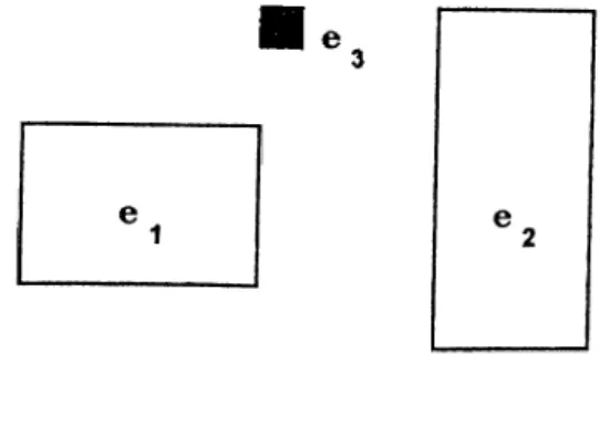
3.1 Old exemplars ®land®2 ₁₆

3.2 N e w exem plar ®3 matches ®1 17

3.3 Match leads to success. Form a generalization ®g 1 7

3.4 Generalization with exception 18

LIST OF TABLES

4.1 Performance results for different Global Future

Adjustment Rates 28

4.2 W eights o f Features with the Rules Generated

for Optimum Global Feature Adjustment Rate 29

CHAPTER I

INTRODUCTION

The high sensitivity o f the capital markets to political and economical events have influenced the efficiency and trend o f the markets over the last decade and brought about sensational variations o f the indices as well as sudden dramatic variations o f trend, thus frustrating the efforts o f some authoritative followers o f one method o f prediction or another. For this purpose a vast amount o f research has been conducted on market efficiency tests in capital markets. However these remarks should not lead the investor to an attitude o f discouragement and helplessness towards the market, but only o f caution, since we believe it is possible, with the help o f adequate decision instruments, to reduce the risks involved to minimum [Pasquale 1991].

Systems for inducing concept descriptions from examples have been one o f the valuable decision instruments for assisting in the task o f knowledge acquisition for expert systems. In this study, we used the theory of learning from examples called Nested Generalized Exemplars (NGE) theory [Salzberg 1990] and applied this neural network and fuzzy computing technology to evolve the software for predicting Istanbul Securities Exchange Composite Index.

Although there has been considerable amount o f studies about the presence o f weak and semi-strong form efficiency at Istanbul Securities Exchange, there has been no published research about the prediction o f ISE composite index using this kind o f a methodology with the historical information reflected in the past prices.

The aim o f this study is to predict the ISE composite index by using the information reflected in the past prices o f some o f the commonly used monetary variables: Central Bank

effective selling price o f US Dollar and DM, Istanbul Tahtakale closing selling price o f Turkish Republic gold coin and one ounce o f gold. Commercial Banks 3 month average deposit rate and 3 month Government bond interest rate.

In Chapter 2, a review o f literature about market efficiency, empirical studies about the efficiency in ISE, and a summary o f research on the predictive ability o f the monetary variables in Turkish Stock Market is presented.

In Chapter 3, the data used in this study are explained. Then we introduce the theory o f learning from examples called Nested Generalized Exemplar and demonstrate its importance with empirical results in several domains. Background about the method, comparison with other exemplar-based theories and econometric models, and types o f generalization are explained. The steps o f the Nested Generalized Exemplar Algorithm: the initialization, fetching the examples, and the matching process o f the algorithm is explained in detail with pseudo codes.

In Chapter 4, modifications made to the original algorithm, its comparison with the simple model, and the findings o f our study from the application o f the algorithm to the Turkish Stock M arket is presented.

Concluding remarks and the results o f the model used is discussed and avenues for further research are presented in Chapter 5. The source code o f the program is presented in Appendix A , setting file in Appendix B and the input data is available in Appendix C.

CHAPTER II

LITERATURE SURVEY

Market Efficiency and the Previous Empirical Work

The early research o f market efficiency hypothesis discussed by [Fama 1970] in his well-known article, pointed out that, a market, which security prices fully reflect all available information is called efficient. Fama, in the 1970 review, divided work on market efficiency into three categories: the 'weak form', the 'semi-strong form' and the 'strong form'.

In a weakly efficient market, present prices reflect all information contained in the record o f past prices, that is, investors cannot consistently earn abnormal returns by observing the past prices. In a semi-strongly efficient market, present prices reflect all available information, that is, security prices adjust rapidly and correctly to the announcement o f all publicly available information. In a strongly efficient market, present prices reflect all information both privately held and insider information together with publicly available information.

The early research [Fama&Blume 1966] proved that developed markets are efficient in the weak and semi-strong sense [Fama 1965] but there is not a consensus in the strong form o f market efficiency hypothesis o f [Jensen 1968] and [Sharpe 1966]. Efficiency literature measures the efficiency o f security markets by testing the predictability o f returns by using certain information sets e.g., past prices, publicly available information, monopolistic information. The recent studies [Zarovin 1990], uses historical price series in order to test the weak form o f efficient market hypothesis. Some o f them used publicly available information and announcements in order to test the semi-strong form o f market efficiency e.g.

[Falk&Levy 1989]. [Chan&Chen 1991] used the behaviors o f investors who have private and insider information in their strong form efficiency tests.

Although research on market efficiency is assumed to be the most successful in empirical economics, with good prospects to remain so in the feature [Fama 1991], information revealed by macroeconomic variables has been ignored in the efficient market literature with few exceptions. However during the last decade, researchers have been interested in macroeconomic variables such as inflation, interest rates, foreign currency, and other term structure (monetary and fiscal) variables [Fama 1991]. In brief, the new work says that returns are predictable from past returns.

Macroeconomic variables are important information sets for developing countries, where application o f financial instruments and institutions are veiy new and the operations in the market is not deep [Moore 1980]. These variables are proved to be efficient indicators o f the market since the investors are not charged for extra costs in collecting these information sets [Mishkin 1982].

Studies [Darrat 1988] on Canadian Stock Market, verifies that a significant lagged relationship between fiscal variables and stock prices is observed. Similarly, Hancock [1989] found that the semi-strong form o f efficient market hypothesis in US stock market is valid for both monetary and fiscal variables. Studies o f Bulmash and Trivoli [1991] investigated the relationship between stock prices and the national economic activity as measured by a series o f key economic variables like money supply, 3-month maturity Treasury bill average yield, 10-years maturity Treasury Bond, Composite Stock Market average. Industrial production rate, unemployment rate. The results o f the statistical analysis o f the hypothesized relationships confirm that there are time lags that transpire between economic variables and stock returns. They provide a new perspective on several studies o f [Fama&French 1988], [Summers 1986], and [Poterba&Summers 1988] that stock prices contain a predictable component and can be predicted by various lagged economic factors.

[Pearce&Roley 1985] examined the daily returns o f stock prices to changes in the money supply, inflation rate corresponding to percentage changes in the Consumer and

Producer Price Index (CPI & PPI), industrial production, unemployment rate, and the discount rate in order to test the efficient market hypothesis that only the unexpected part o f a change in those variables effects the stock returns.

Structure of the Turkish Stock Market

The role o f financial liberalization policies implemented in Turkey affected the monetary and capital market variables and these variables are being considered as the key elements o f this transition process [Gultekin&Sak 1990].

The financial liberalization process in Turkey began in the early 1980s. The concept can be loosely defined as limiting the involvement o f government in the financial markets and giving way to market forces [Sak&Yeldan 1993]. Prior to that time, the Turkish financial system was relatively unsophisticated; commercial banks were the sole suppliers o f funds to users, and loans and deposits, the only available financial instruments. Interest rates were tightly regulated and limited the scope o f bilateral negotiations. Capital movements were strictly controlled. Banks were basically acting as branches o f the government for collecting and distributing surplus funds in the economy. The absence o f an Interbank market to aggregate and transmit the expectations o f economic agents was an additional distorting factor [Atiyas&Ersel 1992].

As for the securities markets, there was literally no activity on the ISE. Although corporations began to issue bonds in the latter half o f the 1970s, there was no orderly secondary bond market. As for government bonds, some o f them were not actually issued but written on the accounts as bonds when the government had to turn to the banking system in times o f liquidity needs. Finally, there was a group o f unorganized securities brokers who traded corporate and government bonds at huge discounts on the face value o f the security [Akjdiz 1988].

The reform process started with the deregulation o f interest rates. Following this first step, foreign exchange regulations were liberalized to ease capital movements. Money and capital markets were introduced into the economy with the objective o f creating collective

markets. With deregulation, banks became relatively free to determine their deposit and loan rates. The deregulation o f interest rates came together with measures on the foreign exchange regulations. Turkish citizens were left free to hold foreign exchange and open foreign exchange accounts with the domestic banks. The ultimate objective was full convertibility o f the Turkish currency [Sak&Yeldan 1993].

The Interbank money market is established to reflect short term scarcity o f resources which is highly volatile. For long term economic decisions, secondary capital markets, especially government and corporate bond markets, became very important variables which produce information reflecting the general expectations o f the longer term trend o f the general economy [Sak&Yeldan 1993].

The ISE was reorganized and began its operations in 1985. The objective was to collect all secondary market activities under the auspices o f the exchange. Mutual funds were defined and established with objective o f creating the institutional demand for the markets. Foreign participation in Turkish securities markets was made possible and easy with investment through collective investment funds. In 1989, foreign portfolio investments on ISE became possible. Although foreign participation gave a boost to the stock market and acted as a catalyst for domestic participation in the market, in a thin market like Turkey, it also increased the volatility o f the market. It made the market very vulnerable to the impact o f foreign exchange rates, especially US Dollar and DM became determinants o f the market.

The allocation o f the private portfolio in Turkey is interest sensitive [Ersel&Sak 1985]. The real rate o f interest plays a crucial role in the portfolio decisions between the domestic and foreign currency substitution. Gold being a non-interest bearing asset, is in competition with fixed interest securities as an investment medium. So, an inverse relationship between the gold price, stock returns and the level o f interest rates should be expected [Gultekin 1986]. Besides interest rates tend to rise during inflationary times and, therefore, gold, as an inflation hedge, and interest rates would move in the same direction.

However, there are some pitfalls; the number o f full-proof economic indicators in Turkey are very few. To develop a forecasting method, recognized human experts are

needed. But professionals in the industry that we consulted tend to agree that there is no acknowledged investment expertise and there is the persistent problem o f finding ways o f focusing on only the relevant facts in a large amount o f data and o f keeping track o f the justifications for beliefs.

Empirical Tests of the Predictive Ability of the Monetary Variables in Turkey

Studies made in this context [§engul&Onkal 1992], tests the semi-strong form o f efficient market hj^pothesis by using certain monetary and fiscal variables as the set o f publicly available information in Turkey. These variables are the monthly growth rate in total amount o f money; TL in circulation plus the sight and time deposits, monthly inflation rate, change in the government budget deficit which is used as the percentage change in the short term loans o f Treasury to the Central Bank o f Turkey, monthly industrial growth rate as an indicator o f GNP, monthly unemployment rate, monthly industry growth rate. Interbank monthly effective interest rate, and money supply. In order to differentiate the expected values and unexpected changes o f the fiscal and monetary variables they used two step approach o f Barro (1977-78). Their test results verify that the market is inefficient; a significant lagged relationship between fiscal and monetary policy and stock returns is observed.

Another study [Erol&Aydogan 1992] tested Arbitrage Pricing Theory Ross [1976] as an asset pricing model to see if asset returns in the context o f the Turkish stock market can be explained by a model which has been tested extensively in well-established capital markets. The pricing effects o f macro-economic variables including the industrial production, inflation, real interest rate, risk premium are tested in the Turkish Stock Market. Pure judgment is used in choosing the variables and in identifying the economic factors that may explain the co­ movement o f stock returns e.g. [Huberman&Kandel 1985]. It is found that the portfolio returns seem to be determined to a great extent by the proposed state variables but it is seen that only the unanticipated part o f those state variables; inflation, real rate and risk premium have significant effects on the return structure o f Turkish Stock Market although it is a new and emerging stock market o f a developing country.

Sönmez and Berik [1993] used the models developed by [Chen&Roll&Ross 1986] and [Fama&Macbeth 1973], to test the significance o f monetary variables in explaining their return behavior on ISE composite index. Briefly, this method regresses the returns on the economic variables o f over an initial estimation period. The resulting coefficients (Beta's) are then used as independent variables in monthly cross-sectional regressions over a later hold­ out period. This generates a time series o f estimates o f risk premium associated with each economic variable. The time-series means o f estimates are then tested by a t-test for statistical significance. The sample range o f the study contains 632 examples starting from the period o f January 1st, 1991 to April 4th, 1993. They used Tahtakale closing selling price o f Turkish Republic gold coin and one ounce o f gold. Central Bank effective selling price o f US Dollars and DM, a basket which contains 50% o f US Dollars and 50% o f DM, 12,9,6 and 3 months o f government bond interest rates, average interest rate on deposits, and overnight Interbank interest rate as the monetary variables to set up the general factor regression equation. The results o f their tests proves that the Turkish stock market is inefficient in the sense that information reflected in the past prices o f those variables have significant effects on ISE composite index. The results indicate that only the Commercial Banks average 3-months interest rate on deposits and overnight Interbank interest rate do not have significant effects on the composite index and should not be included in such a model.

In this study, we used pure judgment o f experts (portfolio managers, dealers and brokers) and the results o f the previous studies in choosing the variables and identifying the economic factors that may explain the co-movement o f stock returns [Huberman&Kandel 1985]. The selected subset o f these commonly used monetary variables are: Central Bank effective selling price o f US Dollar and DM, Istanbul Tahtakale closing selling price o f Turkish republic gold coin and one ounce o f gold. Commercial Banks 3 month average deposit rate, and 3 month Government Bond interest rate.

The purpose o f this study is to use these variables for predicting the ISE composite

index by using Nested Generalized Exemplars which is a model different from previously

CHAPTER III

DATA AND METHODOLOGY

3.1. Data

The data used in this study consists o f 18 months (January 1st, 1991 to June 30th, 1992) o f daily data. For each variable, percentage change in the value o f the variable from the previous day value is calculated for 395 business days e.g. [Pearce&Roley 1985], i.e., 395 examples are used as an input for the algorithm.

First, a literature survey is made in order to identify monetary variables that effect the Turkish stock market and then expert opinions were taken (İş bank, Ankara head office portfolio managers, Hitit Menkul Kiymetler brokers) to identify the variables which reflect the fiscal and monetary changes, to be used at the design stage o f the prediction. By taking the study o f [Erol&Aydoğan 1992] and [Huberman&Kandel 1985] as a reference, we considered the pure judgment o f experts in choosing the variables and in identifying the economic factors that may explain the movement o f stock returns.

The following variables were selected as the commonly used monetary variables to predict stock returns; Central Bank effective selling price o f US Dollar and DM, Istanbul Tahtakale closing selling price o f Turkish Republic gold coin and one ounce o f gold. Commercial Banks 3 month average deposit rate (İş bank, Akbank, Yapı Kredi Bank, and Ziraat Bank 3 months average deposit rate is used because these banks have the highest volume o f time and sight deposits and other operations among the existing public and commercial banks in Turkey) and 3 month Government Bond interest rates. The data used in this study is taken from the Capital Market Board o f Turkey monthly bulletins.

3.2. Comparison of Exemplar Based Learning Model with Econometric Model

The variables are in general complexly related and buried in noise. One advantage o f the NGE algorithm is that it can learn to detect statistical relations hidden in masses o f data which even a human expert would not see.

Compared to Econometric Models (EM), Exemplar Based Learning (EBL), i.e., learning from examples is relatively new, but it plays an important role since it is very effective especially when the amount o f historical data on hand is not sufficient, past data are either no longer relevant or expected to change significantly, and if there is not enough time available to gather and analyze the data [Jain 1987]. Unlike other models o f forecasting; Nested Generalized Exemplars algorithm (NGE) which is a type o f EBL, has two steps to forecasting: first, learning the data and generating rules, second, using the rules to prepare a forecast. The broad distinction between NGE type o f forecasting and EM oriented forecasting is in the generation o f rules from the present data and the process o f judgment. In the broad sense o f the word, judgment is a necessary ingredient o f all types o f predictions.

In NGE, computer is left to make judgments while creating the rules depending on the variables. The selection o f variables becomes very important in this type o f model because after the learning step, giving personal or expertise feedback to the computer will not be possible.

Judgment in EM can enter into the forecasting process at various stages, though its proper role is to be a complement to, not a substitute for, a competent economic and statistical analysis. In NGE algorithm the judgment enters only at the design stage o f the forecast. The understanding o f the judgmental process can be helpful in the development and use o f quantitative techniques. Informed judgment can go far in making forecasts more consistent and dependable. Compared to EM, NGE forecasting explains the significance o f the variables effecting the result o f the forecast but in EM it is also possible to see the cross­ correlation between those variables. It should be recognized that the ability to reach a good judgment is not a well-defined, technical and transferable skill. It is rather a function o f personal experience and training in EM type o f forecasting.

There is enough evidence that mechanical use o f Econometric Models do not produce the most accurate forecasts [Keng 1984]. All the real world forecasts reflect the information o f econometric and pure judgmental inputs.

Forecasting practitioners would probably agree that the speed with which a forecast is generated is important. Econometric models meet this requirement easily. The capability producing timely simulations and o f calculating dynamic multipliers are other important features o f econometric models.

There is enough evidence to support the thesis that human beings are ill-suited to the task o f judging in a probabilistic environment, are poor substitutes for large-scale econometric models when internally consistent forecasts o f numerous variables are needed and it should be noted that human beings have only limited information processing capacity. From this sense NGE algorithm, using computer’s Central Processing Unit (CPU), can handle huge amounts o f processes efficiently, reliably and faster than any other human being.

At present, it is far from clear whether an econometric forecast is superior or inferior to a learning from examples type o f forecast. In some cases, EBL base their forecasts largely on figures produced by econometric methods. If we assume that econometric forecasts are judgmentally adjusted (which is normally the case), then even econometric forecasts contain the forecaster's judgment. In that case, there is no point in discriminating econometric forecasts from the learning based types.

In general, whether or not a forecast will be accepted depends on the user's value. Under the presumption that all forecasters are human beings and they are neither omnipotent nor omniscient. Econometric Models, because o f being used for years and presented it's forecasts to users with a fair amount o f scientific justifications, have the value o f user's. However, N GE is in its infancy.

Exemplar-based learning algorithm is usually developed with the help o f human experts who, by solving specific problems, reveal their thought process as they proceed. After keying into the computer all known information about a particular subject, programmers interview the experts at great length to determine how they use specialized knowledge to form

judgments on fuzzy, non-numerical problems. If this process o f analysis is successful, the computer program based on the analysis is able to solve narrowly defined problems in specialized areas that normally only seasoned experts can handle. The program analyzes the data using the same logic as an expert develops his findings over years o f study and practice.

Exemplar-based learning algorithm, when faced with situations that are complex and unstructured, are considered successful, because it can apply its experience gained in its training phase to solve the problems in an efficient manner. It can employ plausible inference and reasoning from incomplete and uncertain data. It can explain and justify what it does. It does not acquire new knowledge. It restructures and reorganizes the knowledge gained from the data. It recognizes when a problem is outside the boundaries, i.e., exceptions. In essence, it transports chunks o f decision making skill from a human expert's brain to a computer's brain. But it lacks the crucial need for an extensive memory. It is driven by a knowledge-base and judgmental knowledge that is typically made up o f if-then rules.

Exemplar-based learning models solve problems by symbolic inference rather than sequential mathematical calculations done in econometric models [Coats 1987]. It allows for non-numeric tradeoffs and the representation o f judgment. In contrast with the econometric models, this model, when faces with a question for which no answer exists, it applies common sense, and thus does not give up. Instead, it wastes much time searching through its data and rules to come up with a solution.

3.3. Comparison of Exemplar Based Learning Model with other Machine

Learning Models

Exemplar-based learning has only appeared in the literature in the past four or five years, and there are currently veiy few researchers taking this approach. To identify the theory o f NGE, we would like to compare it with the properties o f different Machine learning models.

Knowledge Representation Schemes

Many systems acquire rules during their learning process [Buchanan&Mitchell 1978]. These rules are often expressed in logical form , but also in other form such as schemata [Mooney&DeJong 1985] (i.e. Explanation Based Generalization (EBG) system learns schemata for natural language processing). Usually such systems try to generalize antecedent part o f the rule so that rules will cover larger number o f examples. Another way to represent what is learned, is with decision trees [Quinlan 1986]. Decision trees seem to lack o f clarity as representations o f knowledge; the structure o f the induced trees has been shown to be confusing to human experts, especially when the effect o f one variable is masked by other variables. Rules and decision trees do not exhaust the possible representations o f the knowledge a learning system may acquire. The NGE learning model uses neither o f these representation. Instead, it creates a memory space filled with exemplars, many o f which represents generalizations and some o f which represent individual examples, where the exemplars are hyper rectangles. In addition, it modifies its own distance metric, which it uses to measure distances between exemplars, based on feedback from its predictions. Instead o f generalizing values by replacing symbols with more general symbols, it generalizes by expanding hyper rectangles, which corresponds to replacing ranges o f numeric values with larger ones.

Learning Strategy

In general, there are two categories: incremental and non-incremental (one-shot) learning. NGE falls into incremental learning category so that, it is sensitive to the order o f the examples. The non-incremental learning model offers the advantage o f not being sensitive to the order o f the training examples. However, it introduces the additional complexity o f requiring the program to decide when it should stop its analysis.

Domain Dependency

NGE is domain independent learning algorithm. Because input is simply vector o f feature values and class o f the example. It does not convert examples into another

representational form, it does not need a domain theory to explain what conversions are legal, or even what the representations mean.

Generalization with Exception

Perhaps the most important distinguishing feature o f the NGE is its ability to capture generalizations with exceptions. This is due to the working space (Euclidean) o f the NGE. NGE explicitly handles exceptions by creating hole in the hyper rectangles. These holes (exceptions) are also hyper rectangles and they can have additional exceptions inside them.

Capability of Handling Multiple concepts

Some o f the models that handle multiple concepts need to be told exactly how many concepts they are learning. However, NGE will create as many concepts as it needs. It performs better with a small number o f features as do all learning models. However, it degrades only veiy gradually, as it scales up to larger number o f features.

Different Type of Feature Values

M ost o f the learning models handle only one type o f feature and class values (i.e. binary, discrete, continuous etc.). NGE can handle mixed type o f feature and class values. For continuous values user defined matching tolerance can be used. Humans have remarkable ability to learn from single example, and this ability is one that the NGE model tries to emulate.

Disjunctive Concepts

Many concept learning models have ignored disjunctive concepts [Iba 1979], because they are very difficult to learn. NGE handles disjunctive concepts very easily. It can store many distinct exemplars which carry the same prediction or they describe the same category. An example which matches any o f these distinct exemplars will fall into the category they represent. Set o f such exemplars represent a disjunctive concept.

Inconsistent Data

NGE does not assume that, the exemplars are consistent (i.e. two examples with same feature values but they are in different categories). NGE simply keeps track o f the reliability

o f the exemplars (number o f correct prediction and number o f reference to the exemplar). If N GE faces with inconsistency, it simply reduces the reliability o f the exemplar and will generate new exemplar.

Problem Domain Characteristic

As mentioned before, NGE is domain independent learning algorithm. But it is worthwhile to consider the kinds o f problem domains that are more suitable to NGE. In particular, NGE is the best suited for domains in which the examples form clusters in feature space and where the behavior o f the examples in a cluster is relatively constant or they fall into the same category.

3.4. Methodology

Nested Generalized Exemplar theory is a variation o f a learning model called exemplar- based learning, which was originally proposed as a model o f human learning by Medin and Schaffer in 1978. In the simplest form o f the exemplar-based learning, every example is stored in memory, with no change in representation. Apart from being simple and fast in learning , a major advantage is that no assumptions need to be made since the model is able to extract hidden information from the historical data. Compared to the linear regression method, the neural network produce much more accurate results [Wong&Tan 1991] . However, the performance o f neural networks is affected by many factors, including the network structure, the training parameters and the nature o f the data series [Tang&Fishwick 1991]. NGE adds generalization on top o f the simple exemplar-based learning. In NGE, generalizations take the form o f hyper rectangles in Euclidean n-space, where the space is defined by the feature values for each example. This theory does not cover all types o f learning, rather it is a model o f a process whereby one observes a series o f examples and becomes adept at understanding what those examples are examples o f The algorithm compares new examples to those it has seen before and finds the most similar example in the memory. To determine what is most similar, a similarity metric is used. The term exemplar is used specifically to denote an example stored in computer memoiy. Exemplars have

properties such as weights, shapes and sizes which can be adjusted based on the results o f the prediction. The learning itself takes place only after the algorithm receives feedback on its prediction. If the prediction is correct, the algorithm strengthens the exemplar by increasing its weight, else weakens the exemplar.

It uses numeric slots for feature values o f exemplar. Generalization is a process o f replacing the slot values with more general values (i.e. replacing range o f values [a,b] with another range [c ,d ], where c<a and d>b). The exemplar-based paradigm performs two kinds o f generalization, one implicit and the other explicit.

If an example is stored in the memory with n being the number o f features the system can recognize, then the example is a point in n-dimensional feature space. These points in memory are exemplars. The algorithm uses its similarity metric to compare new examples to the stored exemplars and uses the closest exemplar to make predictions. Thus the exemplars stored in feature space, even when stored as simple points, partition the space into regions, where the region surrounding a particular exemplar contains all points closer to that exemplar than to any other. The similarity metric determines the size and shape o f this region. This generalization process is implicit, since it occurs automatically whenever a new point is stored in feature space.

Figure 3.1: Old exemplars ®1 and

Figure 3.2: New exemplar ®3 matches ®1

Figure 3.3: Match leads to success. Form a generalization .

In NGE model, explicit generalization occurs by turning points into hyper rectangles, and by growing hyper rectangles to make them larger. Explicit generalization in the algorithm begins when a new example falls near two or more existing exemplars. This new point is combined with the closest existing point in memory to form a generalization which takes the shape o f a hyper rectangle; that is, an n-dimensional solid whose faces are all rectangles. The closest existing exemplar may already be a hyper rectangle, in which case it is extended just far enough to include the new point. Figures 3.1- 3.3 provide a graphic illustration o f this process. The generalization ®g includes a larger area than ®1, and replaces the former region in memory.

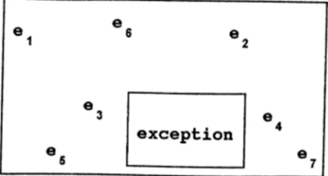
Figure 3.4: Generalization with exception .

If a new example falls inside an existing exemplar region in feature space, but the example behaves differently from others which fell in that same hyper rectangle, the learning system must recognize the new point as an exception. Once the system has recognized that the new point belongs in a different category, it simply stores the point. Prediction failures serve as a signal to the system that a new point does not fit into an existing category. If no more exceptions occur, the point remains a point. However, another exceptional point is found inside the hyper rectangle and if this second exception belongs to the same category as the first one, the two points are combined to create a small hyper rectangle inside the larger one. this new region behaves as an exception to the old generalization. Figure 3.4 illustrates, in two dimensions, what a generalization with a rectangular exception looks like in the feature space.

Once a theory moves from a symbolic space to a Euclidean space, it becomes possible to nest generalization one inside the other. This is where nested comes to the name o f the theoiy. Its generalizations, which take the form o f hyper rectangles in Euclidean n-space, can be nested to an arbitrary depth, where inner rectangles act as exception to the outer ones. This section describes the details o f the nested generalized exemplar learning algorithm. The text below is organized exactly in the order the program functions. Each o f the sections which follows, then, is a phase o f the program's operation. Following the sections describing the individual steps in the algorithm, we give a summary and flowchart o f the algorithm.

In order to make predictions, the algorithm must have a history o f examples on which to base its predictions. Memory is initialized by seeding it with a set o f examples (the minimum size o f this set is one). The seeding process simply stores each example in memory without attempting to make any predictions. An example is a vector o f features, where each feature may have any number o f values, ranging from two (for binary features) to infinity (for real-valued features). In addition , each exemplar has a slot containing the prediction associated with that example. The error tolerance parameter should be used in real-valued variables to indicate how close two values must be in order to be considered a match. This parameter is necessary because for real-valued variables it is usually the case that no two values ever match exactly, and yet the system needs to know if its prediction was close enough to be considered correct. The seed examples are used as the basis o f memory, and memory is used to make predictions. The seeds may be scattered widely or tightly bunched, since they are chosen at random (with small or large number o f seeds, the arrangement or choice o f seeds has little or no effect on the program's learning performance). After initial seeding, the system begins its main processing loop.

3.4.2. Get the next example

The first step in the main loop is fetching the example. It keeps track, for every feature which has numeric values, o f the maximum and minimum values experienced, to scale the features in the distance calculations.

3 .4 .1 . I n itia liz a tio n

3.4.3. The matching Process

The matching process is one o f the central features o f the algorithm. This process uses the distance metric to measure the distance (or similarity) between a new data point (an

example) and an exemplar memory object (a hyper rectangle in n-E). We will refer to the new data point as E and the hyper rectangle as H..

The system computes a match score between E and H by measuring the Euclidean distance between the two objects. Consider the simple case where H is a point, representing an individual example. The distance is determined by usual distance function computed over every dimension in feature space :

D

■ '

“ lower

.

if

E f <

W g : weight of hyper rectanglrj^ ^ ^ k ^ k )

k

W : weight of the future

maXj, min^ : maximum and minimum feature values respectively. E I P : value of the i feature on example E.

m : number of features recognizable on E.

The best match is the one with the smallest distance. A few special characteristics o f the computation, which are not evident in the formula above , deserve mention here. First, let's suppose we measure the distance between E and H along the dimension f Suppose for simplicity that f is a real valued feature. In order to normalize all distances, so that one

dimension will not overwhelm the others, the maximum distance between E and H along any dimension is 1. To maintain this property, the system uses its statistics on the maximum and minimum values o f every feature. Suppose that for E, the value o f f is 10, and for H, the value o f f is 30. The unnormalized distance is therefore 20. Suppose further that the minimum value o f f for all exemplars is 3, and the maximum value is 53. Then the total range o f f is only 50, and the normalized distance from E to H along this dimension is 20/50, or 0.4. Because the maximum and minimum values o f a feature are not given a priority, the distance calculation will vary over time as these values change. This variation is a direct consequence o f the incremental nature o f the algorithm.

N ow consider what happens when the exemplar, H, is not a point but a hyper rectangle, as is usually the case. In this case, the system finds the distance from E to the nearest face o f H. The distance measured by the formula above, is equivalent to the length o f a line dropped perpendicularly from the point E fj to the nearest surface, edge, or com er o f H. This length is modified by the weighting factors. Notice that there are two weights on the distance metric. Wh is a simple measure o f how frequently the exemplar, H, has been used to

make a correct prediction. In fact, the use o f this weight means that the distance metric measures more than just distance. It is a reliability measure, or the probability o f making a correct prediction, o f each exemplar. This weight measure says, in effect, "in this region o f the feature space, the reliability o f my prediction is n", and o f course the algorithm wants to maximize its success rate, so it should prefer more reliable exemplars. The distance metric accomplishes this as follows; suppose in the above example, H had been used for 15 previous predictions, and that it had been correct on 12 o f those occasions. The system will multiply the weight o f the total match score between E and H by 15/12 or 1.25. Thus weight is a non­ decreasing function o f the number o f times an exemplar has been used. If the exemplar always makes correct prediction than the weight will remain at 1. Larger weights will make the rectangular exemplars very distant from new examples.

The other weight measure, wj , is the weight o f the i^^ feature. These weights are adjusted over time. Since the features do not normally have equal predictive power, they need to be weighted differently

I f the algorithm above, makes the correct prediction, it records some statistics about its performance and then makes a generalization. Two objects E and H are used to form the generalization. H is replaced in memory by a larger object that is a generalization o f E and H. H may have been a single point, or it may have been a h)T)er rectangle. (After a single generalization, an exemplar becomes a hyper rectangle.) If H was a hyper rectangle, then for every feature o f E which did not lie within H, H is extended just far enough so that its boundary contains E. If H and E were both points, H is replaced by a new object which, for each feature o f E and H, a range o f values defined by E and H. For a simple case with just tw o features fi and f2 if E was at (2,5) and H was a point at (3,16), then the new object

would be a rectangle extending from 2 to 3 in the fi dimension and from 5 to 16 in the f2

dimension. If an example falls within an area where two hyper rectangles overlap, the system matches it to the smaller exemplar, because larger exemplars may have been over­ generalized.

3.4.3.2. Incorrect Prediction

I f the system makes the wrong prediction, it has one more chance to make the right one. The idea is to keep down the size o f the memory. Before creating a new exemplar, the algorithm first looks at the second best match in memory. Assume that Hj was the closest exemplar to E and H2 was second closest. If using the second best match, H2, will give the

correct prediction, then the system tries to adjust hyper rectangle shapes in order to make the second closest exemplar into the closest exemplar. It does this by first creating a generalization from H2 and E. It then specializes the best matching exemplar. Hi, by reducing

its size. It reduces the size o f H i, which must be a hyper rectangular (if not, then the system does nothing), by moving its edges away from the new exemplar just far enough so that H2

becomes closer along that dimension. This process is basically a stretching and shrinking operation; H2 is stretched, and Hi is shrunken, in order to change the order o f the match the

next time around. The goal o f this process is to improve the predictive accuracy o f the system

3 .4 .3 .I . C o r r e c t P r e d ic tio n

without increasing the number o f exemplars stored in memory. Shrinking an existing exemplar loses information.

A very important consequence o f this second chance heuristic (referring to the second closest exemplar) is that it allows the formation o f hyper rectangles within other hyper rectangles. If a new point pi lies within an existing rectangle, its distance to that rectangle will be zero. Its distance to another point p2 (previously stored exception) within the rectangle will

be small but positive. Thus the algorithm will first assume that the new point belongs to the same category as the rectangle. If pi is in the same category as p2, then the second chance

heuristic will discover this fact, and form a rectangle from these two points.

If the second best match also makes wrong prediction, then the system simply stores the new example, E, as a point in memory. Thus E is made into an exemplar which can immediately be used to predict future examples, and can be generalized and specialized if necessary. This new exemplar may be inside an existing exemplar H, in which case it acts as an exception to, or hole in H.

The algorithm adjusts the weights wj on the features fj after discovering that it has made the wrong prediction. Weight adjustment occurs in a very simple loop : for each fj, if E fj matches H fj, the weight wj is increased by setting wj = wj (1 + A f ), where A f is the global feature adjustment rate. An increase in weight causes the objects to seem farther apart, and the idea here is that since the algorithm made a mistake matching E and H, it should push them apart in space. If E fj does not match Hf·^ then wj is decreased by setting wi = w, (1 - A f ). If the algorithm makes a correct prediction, feature weights are adjusted in exactly the opposite manner; i.e., weights are decreased for features that matched, which decreases distance, and increased for those that did not. Each weight wj applies uniformly to the entire feature dimension fj, so adjusting wj will move around exemplars everywhere in feature space.

3 .4 ,4 .

Take the two closest hyper rectangles to example

D

EH

and

D..

mini min 2

for

H

H

if H . , .class == E .class then

mini

begin

H

H

Generalize H . . with E in all feature dimensions_{min 1}

end

else if H .

.class == E .class then

mm2

begin

H . , .reference ++

H . , .correct ++

H . . .reference ++

Generalize H . . with E in all feature dimensions

mm2

end

H

Store E as new exemplar

adjust all features weights as follows

if E f matches with

H .

1. mml^

i

else

i

i

end

GOTO Step 2 (get new example, if no more exit)

: is global feature adjustment rate.

CHAPTER IV

FINDINGS

4.1. Modifications to the Algorithm

As mentioned in properties o f the NGE algorithm, main purpose is in learning the correct prediction o f the example. There are some possible modifications to the NGE;

1. Reducing the sensitivity o f the algorithm to the order o f examples. To achieve this, we can do simple modification such that, for initial exemplars instead o f taking first a few examples blindly, we can choose initial exemplars from training set according to average feature values. It will help us to start at a better position.

2. Second issue is reducing the number o f rules which are redundant so that resultant rules can be criticized by human experts. Hence, resultant rules should be compact.

We can explain the modified NGE after pointing out the above issues. New algorithm consists o f two phases: First Phase is same as original NGE. Second Phase o f the algorithm tries to reduce number o f exemplars (generated in first phase) by eliminating the redundant rules.

(1) . Sort (descending) the exemplars according to their reliability (1/ W^).

(2) . If H ci overlaps with H c2 and C1O C2 then

shrink hyper rectangle which has small (1/ Wjj) value.

(3) . Remove the redundant hyper rectangles (i.e. Hi is in H2 and both have same classes.

This can happen due to the generalization).

(4) . Mark the exceptions hence, no more processing is done for exceptions.

(5) . List the rules and than stop.

4.2. Application of the Algorithm to the Stock Market

When an institutional investor has to make a decision on whether and how to act on the stock and bond markets on which he usually operates, he has to take into account a large number o f factors which influence his choice. It has never been as difficult as over the last few years to operate on the financial markets all over the world, as well as to venture predictions on their future trend [Pasquale 1991].

It is not possible to consider all the variables that effect the stock returns, because there is no clear distinction between economical activities. There are some external effects which has to be considered in evaluation process, (insider trading, rumors, other economical activities, alternative markets, political effects, macro economical conjuncture, sector conjuncture, psychological effects etc.). Although these variables could be used for computer representation and processing, we could not find relevant data for these indicators. In this study we used a greatly simplified model o f the Stock Market.

We analyzed the daily percentage in the ISE composite index o f the 395 examples. 12% o f the data were belonging to changes o f more than 3% increase in the ISE composite index. 11% belonging to changes o f more than 3% decrease in the composite index, 77% belonging to increase and decrease between 3%. The maximum decrease on the ISE composite index during this period was observed to be 10.19% and maximum increase was 10.32%. The daily changes in the composite index were commonly very close and between 3% deviations and the average change in the ISE composite index was 0.1269 which shows the increasing trend o f the Turkish Stock Market. The maximum increase and decrease for the variables used during this period were: Turkish Republic Gold Coin; maximum increase 5.17%, maximum decrease 4.06%. Respectively, 9.05% and 6.70% for one Ounce o f Gold, 4.02% and 3.64% for US Dollar; 4.19% and 5.72% for Deutsche Mark, 7.18% and 6.51% for Government Bond Interest Rate, finally 5.30% and 4.67% for Commercial Banks' Average Deposit Rate. Therefore, we defined three classes representing the trend o f the composite index:

1. ISE Composite Index will increase more than 3% (class Cj).

2. ISE Composite Index will decrease more than 3% (class Ca).

3. ISE Composite Index (daily returns) will be between -3% to +3% (class C3).

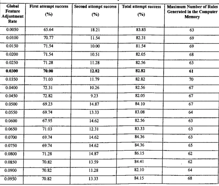
The package uses only historical data for training in the selected field, and no other explicit rules are needed. The program generates rules to the user to make his/her decision. The performance results o f the program run are listed on Table 4.1 for twenty different values o f Af ( the global feature adjustment rate). As it is seen from Table 4.1, the best global feature adjustment rate turns out to be Af = 0.030 for this set o f data since it generates minimum number o f rules with the maximum first attempt correct prediction value.

The first column o f the table shows different values o f global future adjustment rates that are used to identify the most appropriate value. In order to find the best prediction performance o f the algorithm with different values o f global feature adjustment rates, we used 5 o f 395 examples to seed the initialization process and the remaining 80% (312 examples) are used to train the algorithm and the rest, 78 examples, are used to test the algorithm. Second column o f Table 4.1 shows the test results o f making a correct prediction (the class o f the example on hand is same with the class o f the closest rectangle in the memory, e.g., index increase more than 3% as class c l) when algorithm tries to generalize the example on hand with the closest rectangle in the memory. The ratio is calculated as follows: the total number o f correct predictions made to the closest rectangle in the memory / total number o f data used during the test * 100. Third column similarly shows rate o f successful prediction o f the index at the second attempt (when the closest rectangle class does not match with the class o f the example on hand, try to generalize with the second second closest rectangle in the memory). The fourth column o f the table presents the total performance o f the algorithm for predicting the stock market index (second column plus third column). Last column o f Table 4.1 shows the maximum number o f rules generated in the memory.

Table 4.1: Performance Results for different Global Future Adjustment Rates Global

Feature Adjustment

Rate

First attempt success

( % )

Second attempt success

( % )

Total attempt success

( % )

Maximum Number of Rules Generated in the Computer

Memory 0.0050 65.64 18.21 83.85 63 0.0100 70.77 11.54 82.31 69 0.0150 71.54 10.00 81.54 69 0.0200 71.54 10.51 82.05 68 0.0250 71.28 11.28 82.56 63 0.0300 70.00 12.82 82.82 61 0.0350 71.03 11.79 82.82 70 0.0400 72.31 10.26 82.56 67 0.0450 72.82 9.23 82.05 67 0.0500 69.23 14.87 84.10 67 0.0550 69.74 13.33 83.08 64 0.0600 67.95 14.62 82.56 63 0.0650 71.03 12.31 83.33 63 0.0700 69.74 14.62 84.36 63 0.0750 69.74 14.62 84.36 65 0.0800 71.28 14.87 86.15 62 0.0850 70.82 13.59 84.41 62 0.0900 70.82 11.28 82.10 64 0.0950 70.82 13.33 84.15 68

Table 4.2 displays the set o f rules that correspond to the global adjustment rate 0.030. For each feature, two values are given, labeled lower and upper, that describe the allowable percent change in that attribute.

Table 4.2 Rules Generated for Global Feature Adjustment Rate = 0.030. F eatures _Turkish Republic Gold Coin One Ounce of Gold

us

B oundary Low er Upper Low er U pper Lower Upper Lower Upper Lower Upper Lower U pper CF Class R ule 1 -3.70 -2.88 -1.06 -0.93 -0.67 -0.61 -0.75 -0.41 0.00 0.00 0.00 0.00 6/11 c l R ule 2 -3.70 -2.88 -1.53 -1.16 -0.67 -0.61 -0.75 -0.75 0.00 0.00 0.00 0.00 5/8 c l R u le 3 -3.70 -2.88 -3.65 -1.87 -0.95 -0.95 -0.75 -0.75 0.00 0.00 0.00 0.00 3/7 c l R ule 4 -3.70 -2.88 -0.64 -0.53 0.12 0.17 -1.26 -0.75 0.00 0.00 0.00 0.00 2/4 c l R u le s 0.82 0.82 1.36 1.36 0.51 0.51 1.95 1.95 0.00 0.00 0.00 0.00 2/4 c l R u le 6 -3.70 -2.88 -0.64 -0.53 0.40 0.42 -0.75 -0.41 0.00 0.00 0.00 0.00 2/4 c l R u le ? -3.70 -2.88 -0.84 -0.65 -0.67 -0.61 -0.75 -0.75 -2.72 -2.04 -0.11 -0.03 2/3 c l R ule 8 -4.06 -4.00 -0.93 -0.64 -0.67 -0.61 -0.75 -0.75 0.00 0.00 0.00 0.00 2/4 c l R ule 9 -3.70 -2.88 -2.33 -1.87 0.00 0.11 -0.75 -0.75 1.44 6.84 -0.36 -0.11 Ш c2 R u le 10 1.16 1.16 0.48 0.48 0.11 0.11 -0.75 -0.75 0.00 0.00 0.00 0.00 1/2 c2 R ule 11 -3.70 -2.88 -1.05 -1.05 -0.23 -0.23 -0.75 -0.41 0.00 0.00 0.00 0.00 1/2 c2 R ule 12 -3.70 -2.88 -0.64 -0.53 0.11 0.11 -0.75 -0.75 0.00 0.00 0.16 0.16 1/2 c2 R ule 13 -3.70 -2.88 -0.64 -0.53 0.56 0.56 -0.75 -0.75 0.00 0.00 0.00 0.00 1/2 c2 R ule 14 -3.70 -2.88 -1.58 -1.58 -0.94 -0.94 -0.75 -0.41 2.14 2.14 0.05 0.05 1/2 c2 Rule 15 -3.70 -2.88 -0.64 -0.56 -0.67 -0.61 -0.75 -0.41 0.00 0.00 0.00 0.00 1/3 c2 R u le 16 -3.70 -2.88 0.47 0.47 -0.67 -0.63 -0.75 -0.41 0.00 0.00 0.00 0.00 1/2 c2 R ule 17 0.80 0.80 0.80 0.80 0.21 0.21 -0.75 -0.41 0.00 0.00 0.00 0.00 1/2 c2 R u l é i s -3.70 -2.88 -0.64 -0.53 0.41 0.41 -0.75 -0.41 0.00 0.00 0.00 0.00 1/2 c2 R ule 19 -3.70 -2.88 -0.64 -0.53 -0.10 -0.10 -0.75 -0.75 0.00 0.00 0.00 0.00 1/2 c2 Rule 20 0.78 0.78 0.53 0.61 0.20 0.20 -0.75 -0.41 0.00 0.00 0.00 0.00 1/2 c2 Rule 21 -3.78 -2.88 -0.64 -0.53 0.20 0.20 -0.75 -0.41 0.00 0.00 0.00 0.00 1/2 c2 R ule 22 -3.70 -2.88 -0.64 -0.53 -0.30 -0.30 -0.75 -0.41 0.00 0.00 0.00 0.00 1/3 c2 Rule 23 2.40 2.40 1.89 1.89 -0.16 0.00 -0.75 -0.41 0.00 0.00 0.00 0.00 1/3 c2 R ule 24 1.02 1.02 0.93 1.03 0.50 0.50 -0.75 -0.41 0.00 0.00 0.00 0.00 1/2 c2 R ule 2 5 -3.70 -2.88 -0.64 -0.53 0.00 0.00 -0.75 -0.41 0.00 0.00 0.00 0.00 1/3 c2 _R ule 26 -3.70 -2.88 -1.28 -1.28 -1.34 -1.34 -0.75 -0.41 0.00 0.00 0.00 0.00 1/2 c2 R ule 27 -3.70 -2.88 -0.64 -0.53 0.29 0.29 -0.75 -0.41 0.00 0.00 0.00 0.00 1/2 c2 R ule 28 -3.70 -2.88 -0.76 -0.76 -0.38 -0.38 -0.75 -0.41 0.00 0.00 0.00 0.00 1/2 c2 R ule 2 9 -3.70 -2.88 -0.65 -0.65 0.37 0.37 -0.75 -0.41 0.00 0.00 0.00 0.00 1/1 c2 R ule 3 0 -3.70 -2.88 -0.64 -0.53 0.27 0.27 -0.75 -0.41 0.00 0.00 0.00 0.00 1/2 c2 R ule 31 -3.70 -2.88 -1.08 -1.08 -2.22 -2.22 -0.75 -0.41 -2.72 -1.86 0.00 0.00 1/1 c2 Rule 32 -3.70 -2.88 -0 .6 4 -0.53 0.33 0.33 -0.75 -0.41 0.00 0.00 0.00 0.00 1/2 c2 R ule 33 -3.70 -2.88 -0.64 -0.53 0.00 0.00 -0.75 -0.41 2.17 2.17 0.00 0.00 1/1 c2 Rule 34 -0.50 0.00 -0.47 -0.15 -0.67 -0.39 -0.58 -0.29 -1.15 0.00 -0.11 0.00 18/46 c3 _ R u le 3 5 2.87 5.17 0.53 0.75 0.68 0.80 .0.29 -0.23 0.00 0.00 0.00 0.00 4/6 c3 R ule 36 0.28 0.64 -0.53 0.45 -0.51 -0.45 0.55 0.80 0.00 0.00 0.00 0.00 3/5 c3 R ule 37 2.02 2.02 0.93 1.35 0.17 0.17 -0.75 0.00 0.00 0.00 0.00 0.00 2/5 c3 Rule 3 8 0.37 0.37 0.00 0.00 0.00 0.00 0.00 0.00 0.00 0.00 0.00 0.00 1/2 c3 R ule 3 9 -0.69 -0.69 0.00 0.00 -1.91 -1.91 -1.31 -1.31 0.00 0.00 0.00 0.00 1/2 c3 R ide 40 -3.70 0.78 -0.64 0.39 0.66 0.66 -0.75 0.60 0.00 1.13 0.43 0.43 1/5 c3 Rule 41 -2.88 -2.88 0.49 0.49 0.56 0.56 -0.21 -0.21 6.84 6.84 5.30 5.30 1/1 c3 _R ule 42 -0.32 -0.32 -0.11 -0.11 -1.95 -1.95 -0.41 -0.41 0.00 0.00 0.00 0.00 1/1 c3 R ule 43 -3.71 -3.71 0.69 0.69 0.00 0.00 0.00 0.00 0.00 0.00 0.00 0.00 1/2 c3 Rule 44 0.00 0.00 0.29 0.29 0.11 0.11 -0.39 -0.39 0.00 0.00 0.00 0.00 1/2 c3 ^ R u le4 5 0.56 0.56 0.66 0.66 0.42 0.42 1.45 1.45 0.00 0.00 4.04 4.04 1/2 c3 Rule 46 -1.40 -1.40 -1.87 -1.87 0.00 0.00 -0.36 -0.36 0.00 0.00 0.00 0.00 1/1 c3 _^Rule 47 0.50 0.50 0.42 0.42 -0.20 -0.20 4.19 4.19 0.00 0.00 0,00 0.00 1/1 c3 _R nle 48 -0.74 -0.74 -1.16 -1.16 0.29 0.29 0.00 0.00 0.00 0.00 0.00 0.00 1/2 c3 _R ule 49 0.00 0.00 0.00 0.00 0.53 0.53 0.28 0.28 0.00 0.00 0.00 0.00 1/2

_iL_J

_ ¿ J