Investments viewed as growth processes

THE ENGINEERING ECONOMIST• FALL 1995 • VOWME 41, No. 1

INVESTMENTS VIEWED

As

GROWTH PROCESSES

HALiM DOGRUSOZ

Bilkent University, Turkey

NE.TAT KARABAKAL

University of Michigan

ABSTRACT

1

For modeling investment decision situations, we present a mathematical basis that views the cash flow sequences as growth processes. We first emphasize the pedagogi-cal value of the basic model by showing that all traditionally established measures of worth (profitability) as well as the compound interest formulas of financial mathe-matics can actually be derived from it by simple algebraic manipulations. Then, we argue that the traditional measures fail to recognize the particularities of certain deci-sion situations and point out the need for developing tailor made measures for each specific problem. We demonstrate, using real life examples, our approach for devel-oping new measures and, by incorporating decision variables, practical optimization models from this mathematical basis.

INTRODUCTION

A major group of investments utilizes capital resources. These investments, usually characterized by major cash outflows, are used to acquire production facil-ities that, in turn, generate cash inflows. Furthermore, capital can be borrowed and excess cash can be lent, both for a fee called interest. This seemingly com~ plex process can be viewed as a simple growth process of cash {or capital) since, by its very nature, cash inflows exceed cash outflows. To represent this growth process, in this paper, we present a mathematical basis for modeling investment decision situations.

In evaluating investment alternatives, the question of measure of worth {profitability) has always been a delicate and sometimes controversial issue, even under the assumptions of certainty. Difficulty arises from the fact that benefits obtained and resources expended take place at different points of time over a long stretch of time. This issue is usually introduced symbolically as the time value of money in financial analysis and engineering economy textbooks, meaning that time of acquisition {or spending) has an effect on the value of money ac-quired (or spent) (see, for example, [121). The concept of present value is an in-genious invention which opens up an avenue to resolve the issue. The roots of the concept can be traced back in the early works of Fish [9], Fisher [10], Grant [11], and Hirshleifer [13].

2 THE ENGINEERING EcoNOMIST • FALL 1995 • VOLUME 41, No. 1

In spite of the widespread use of the present value and other measures derived from it, controversy and discussion still continue on the consistency of these measures. See [2] for a comparison, and [16] for a recent review of this literature. The treatment proposed here is hoped to shed some light on the origins by estab-lishing a common mathematical basis from which all these traditionally known measures as well as the compound interest formulas of financial mathematics can be derived. Such a development has a pedagogical value and provides an alterna-tive viewpoint to the usual textbook derivations. However, through an innova-tive use of this basis, the main contributions of the paper are:

1. to construct investment decision models that incorporate the decision (or, design) variables whose values are to be optimized with respect to a cho-sen measure,

2. to derive nontraditional measures of worth for evaluating certain invest-ment alternatives where traditional measures prove inadequate, and hence, 3. to provide a unified framework for the mathematical modeling of

invest-ment decision situations.

The plan of the paper is as follows. First, we introduce the general growth model and show that all the compound interest formulas of financial mathemat-ics can actually be derived from it Next, by defining the concept of equivalence among growth processes, we derive all basic traditional measures of worth com-monly used in the literature. Then, we extend the growth model to include some decision variables and present a prototype optimization framework. We illustrate the use of this framework on an example investment decision problem taken from the petroleum industry. We also discuss and demonstrate, using real life examples, how to develop new measures based on our proposed approach for some investment decision situations where traditional measures are not suitable. Finally, we give our concluding remarks.

DEVELOPMENT OF THE GROWTH MODEL

We conceive the growth process as composed of two interacting sub

pro-cesses:

1. productive growth, and 2. reproductive growth.

Production can be positive or negative, i.e., production is either the cash inflow (positive production) or cash outflow (negative production) resulting from the

TllE ENGINEERING ECONOMIST• FALL 1995 • VOUJME 41, No. 1 3 operation of the system. Reproduction also can be positive or negative in the sense that excess cash reproduces cash through investment (positive reproduc-tion) or cash deficit financed by loans reproduces itself with accrued interest (neg-ative reproduction). These reproductions correspond to interest earned or paid as typical examples.

Now, let x be the cash position of the growth process at a point of time. The variation of x in time t can be represented by the following differential equa-tion:

dx

dt=ax+a.

(1)

The left hand side of equation (1), derivative of x with respect to time t, is the rate of change in x. This rate of change is equated to the sum of two terms. The first is the rate of reproduction and the second is the rate of production. Here,

a

and a can both be functions of time. The reproduction rate (

a

x ) is proportional to x, and its proportionality factor a can be termed unit reproduction rate. Its dimension is dollar per dollar per unit time (as x is measured in terms of dollars). Here, a can be interpreted as interest rate, and a as the rate of cash flow. Obvi-ously, the dimension of a is dollars per unit time.

Equation (1), which models the growth of cash due to investment, is based on the following assumptions.

1. Products, services and inputs are measured with monetary units; i.e., these are represented by the net cash flow rate a.

2. Any cash credit is reinvested and any cash debit is financed by loans. 3. Both reinvestments and loans, earn and cost the same rate.

Thus, equation (1) represents a continuous growth in time, therefore, we call it the continuous time growth equation. Its discrete growth equation can be readi-ly constructed as follows:

x

1 =(l+a,)x,_1

+a,.

(2)

Here, x1 denotes the cash position at the end of time unit t (end of year cash

posi-tion, for example). This difference equation can be put to the following similar form as in equation (1)

4 THEENGINEERINGEcONOMIST•FALL 1995• VoUJME41,NO. l where Ax,

=

x, -

x,-1,

the growth increment in time unit t.

Equation (1) is a fmt order linear differential equation whose solution can readily be obtained as:

(4)

Equation (4) expresses the cash position of the investment situation at the point of time t where Xo is the value of x at time t = 0. In a typical investment situa-tion, xo is negative and represents the initial investment, say /. This equation is what we call the continuous growth model of the investment situation. Here,

cash flow rate a and unit reproduction raie

a

are taken to be functions of time in general. If a is constant, equation (4) becomes:

For constant cash flow rate a, equation (5) becomes even simpler:

We get the discrete time analog of equation (4) as a solution to

equation (2) as:

(5)

(6)

(7)

This is the analogous discrete growth model. Similarly, for constant unit

repro-duction rate

a,

equation (7) becomes:

x,

=

(xo

+

±an(l

+

a)-n)

(1

+a)'.

n=l (8)

Furthermore, for constant cash flow rate a, the following closed formula is ob-tained:

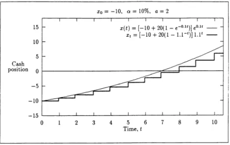
THEENGINEERINGEcONOMIST•FALL 1995• VOUJME41,No. l .5 The continuous growth model represents a growth which talces place every moment of time, and discrete growth model represents a growth which talces place by discrete increments at discrete points of time. A graphical representation for a typical invesbnent situation is given in Figure 1 for both models (equa-tions (6) and (9)). As it is seen in Figure l, for the same values of a= 0.1 and a= 2, x(t)>x,. It can be shown that this property holds in general. However, if

we define Cl= ln(l+a)

=

ln(l.1)

=

0 0953 and Q =(a/a) X a= (.0963/.1) 2

=

1.906, where

a

and a are the values for the discrete case, and substibJte them in the continuous case, we obtain x(t) = x I for the discrete values oft.

All formulas of financial mathematics can be derived from equation (4) and equation (7) which are solutions of equations (1) and (2). Therefore, we like to call them the fundamental equations of financial analysis. Let us demonstrate by

deriving a couple. In the following examples, continuous and discrete versions are given side by side, continuous on the left and discrete on the right

Cash 15 10 5 x0 = -10, c, = 10%, a= 2 x(t) = (-10 + 20(1 - e-0_-lt)J e0 ·1t -x, = [-10 + 20(11.1')] 1.1' -position o 1---:::::::,,;;:=a;a=::lf---i -5 -10 -15 '---''---'---'---'---'---'---...___~~~~~ 0 2 3 4 .5 6 7 8 9 10 Time,t

6 'IHEENGINEERINGECONOMIST•FALL 1995• VOLUME41,NO. l

ExAMPLE. Single payment, compound amount formula, with a

=

0 and

a

=

constant:

x

=

x0e0fl, x, =xo(l+a)'.

EXAMPLE. Uniform cash flow series compound amount formula, with

.xo=

0, a = constant, and

a

= constant:

where the uniform cash flow series is spread over the closed interval [0,h ]. More familiar forms can be obtained by straightforward algebraic simplifications as follows.

((l+a)h-1)

Xh=a .

a

These are well known future value formulas of uniform cash flows in continuous and discrete compounding. Note that, in all these derivations, discrete versions can be obtained from continuous versions by simply substituting (1 +

a )

for

ea and vice versa.

Obviously, formulas can be derived for any functional form of production rates a(t) (cash flow rate) or q (cash flow series) from equation (4) and equation (7), respectively. The main purpose of these equations, however, is to guide the construction of decision models for investment situations, by appropriately in-corporating the so called decision variables. Methodology for this will be devel-oped in subsequent sections.

In the following developments, we assume continuous time growth since it provides a more powerful and convenient mathematical basis as well as it usual-ly approximates real life situations better. Except investments in the capitai market, practically all systems work continuously, and result in both continuous cash flows and continuous reproduction; however, the determination of cash flow production rate and unit reproduction rate requires some subtle work.

REMARK. In developing this growth model, assumption 3 stated above could be relaxed, i.e., different earning rates for reinvestment and loans could be allowed. This, however, would involve a more complex mathematical treatment which could make the application difficult in practice, since it would require distinguishing the time intervals when x > 0 and x < 0.

EQUIVALENCE OF GROWTH PROCESSES

We first define some seemingly familiar but contextually different concepts: horizon, equivalence of capital growth processes, and standard growth processes.

THE ENGINEERING ECONOMIST• FALL 1995 • VOLUME 41, No. 1 7

DEFINITION 1 (Horizon). A fixed arbitrary point of time, H, in the future. Now, consider the size of cash, F (a, H), reached at horizon H, generated by an invesbnent situation with constant unit growth rate of reproduction

a,

F(a,H) =

(xo

+

J:

ae-aldt)ea11.

Call this F(

a ,

II) future value of the growth process.

DEFINITION 2 (Equivalence of two growth processes). A growth process G1 is

called equivalent to another growth process G 2 relative to

a

and H if and only if

their respective future values F1( a ,HJ and Fi( a ,HJ are equal; i.e.,

Fi

(a, H)

=

Fi

(a, H).

Note that equivalence is a property which depends upon the pair (

a

,H); that is, two growth processes equivalent for a given (

a

,H) pair may not be so for another pair (we will see later that under special circumstances equivalence may be invariant).

In order to define a measure of worth for every invesbnent alternative, we need a "standard growth process" equivalent to the one we wish to evaluate. For this purpose, we define two standard growth processes as follows.

DEFINITION 3 (Standard Growth Process I, or Pure Reproductive Process).

Growth process with a = 0,

=

constant,

DEFINITION 4 (Standard Growth Process II). Growth process with a = constant,

a

= constant, and x o = 0,

a (l -al) al

x=-

-e

e .

a

Future values, F1 (

a

,HJ and F11(

a

,H), of these growth processes can readily be obtained as follows:

-e a11 -e a11

(1

-all)

(1

-all}

8 THE ENGINEERING ECONOMIST• FALL 1995 • VOLUME 41, No. 1

given the pair ( a ,H).

In these growth processes, a single parameter -P for the first and A for the

second- can be viewed as their respective measures of worth. We can use these real numbers as measures of worth for a given arbitrary growth process equiva-lent to standard I or II.

Now, consider an investment situation and its future value F(

a,

H ), where:

and its equivalent standard I. By definition: F₁(a, H)

=

F(a, H),

(10) which leads to:

(11)

We call P, given by equation (11), the present value of the investment situation considered. It is a measure of worth since it is equivalent to having capital equal

to P at time zero which grows to F (a, H ) at time H with

a

unit reproductive rate.

Similarly, considering the equivalent standard II, by definition, we write:

F/l(a, H)

=

F(a, H),

A=P(

_1-e

a_uH)·

(12)

(13)

We call A, given by equation (13), the equivalent constant production rate (con-stant cash flow rate) of the investment situation considered. It is a measure of worth since it is equivalent to earning A amount of money per unit time which grows to F (a, H ) with a unit reproductive rate over the time interval [0, H ]. The widely used term in the literature for A is "annual worth" assuming "year"

THE ENGINEERING EcONOMIST• FALL 1995 • VOUJME41, No. 1 9 as the time unit, but for the sake of generality, we prefer "equivalent constant production rate."

We regard P and A as measures of worth for the investment alternatives, since they are "order preserving." That is, an alternative with a larger Pis pre-ferred to the one with a smaller P; similarly for A. These are good measures of worth since they also have intuitive appeal.

We note that both P and A are dependent on the pair (

a

JI). In other words, they are relative to ( a ,II). Therefore, they should be understood as functions of ( a ,II), such as P( a ,H) and A( a ,H). We also see that,

A=P(

_1-e

':@1)•

F(a,H)= Peall.

Hence, we can ~so consider F(

a

,H) as a measure of worth. Since every one of these measures can be expressed in terms of the others, to consider one is equiva-lent to considering any other two. Present value, however, is more popular.

At this point, it may be useful to notice some properties of these measures.

REMARK 1. Consider a production (or cash flow) function a(t) such that a(t) = 0 fort> T. In this case, it is easy to show that P(

a

,H) is invariant with

H > T. For A (

a

,H), however, such a property does not hold. In fact, under this condition

is independent of H, but

is not. Note, however, that A(

a

,H) converges to

a

P, the reproductive growth

rate of capital P, as H tends to infinity.

REMARK 2. All these developments imply the following useful and easy-to-prove property: Two growth processes are equivalent if and only if their respec-tive present values are equal. We utilize this property in the subsequent section to derive new measures.

Two other traditional measures, payback period, Ho, and internal rate of return,

a

0, can readily be obtained as the solutions to

10 THE ENGINEERING ECONOMIST• FALL 1995 • VOLUME 41, No. 1

F(a, II)

=

0 or P(a, H)

=

0,

if they exist. The payback period is used as a surrogate measure for evaluating the risk and the liquidity of the investment alternative rather than a measure of

profitability and is not at all consistent with the above measures [6]. Weingartner [19] suggests it to be used as a measure constrained from above for the acceptability of an investment It is a "satisficing" upper bound in the A. H. Simon sense [17]. Internal rate of return, on the other hand, is consistent with the above measures if used properly. However, its proper use requires a priori

knowledge of the invesbnent type for resolving the multiple root problem and calls for incremental analysis in case of mutually exclusive alternatives. The reader is referred to the references for more details [5, 8, 14, 15].

A PROTOTYPE INVESTMENT DECISION MODEL

In this section, we present a most elementary investment decision model, a mathematical structure, to enable the decision maker to evaluate investment al-ternatives which are represented by decision variables. The model considers the single pfoject case. A composition of the values of the decision variables consti-tutes an investment alternative. For notational convenience, let d = ( d1, d2,

d3, ... ) denote an invesbnent alternative, as an element of the cartesian product D

=

IJi

X

Dz

X

D.3

X ... ; d E D

where D; denotes a set of alternatives, and d; (decision variable) an element of it, for a given characteristic (attribute) of the system to be created by the investment concerned. AD; can be a set of technologies, or a set of locations, or a set of capacities, etc. The nature of the growth process established by the system creat-ed is bascreat-ed on:

](d) - the invested capital disbursed at time t = 0 as a function of d, a(d,t) - production rate as a function of d and obviously may be varying in

time t,

a

(t) = unit reproduction rate which may be varying in time t,

T

=

time of abandoning and scrapping the system, and

S(d,T)

=

salvage value of the system at time T, usually decreasing as Tin-creases.

Here, T can be a decision variable to be optimized (as in the replacement prob-lems), or a priori determined, or imposed by the nature of the system concerned so that it becomes a parameter. Note that most of the decision variables can be

1)IEENGINEERINGECONOM1ST•FALL 1995• VOLUME41,No. l 11

decision making can be viewed as designing a system to be created by the invest-ment concerned

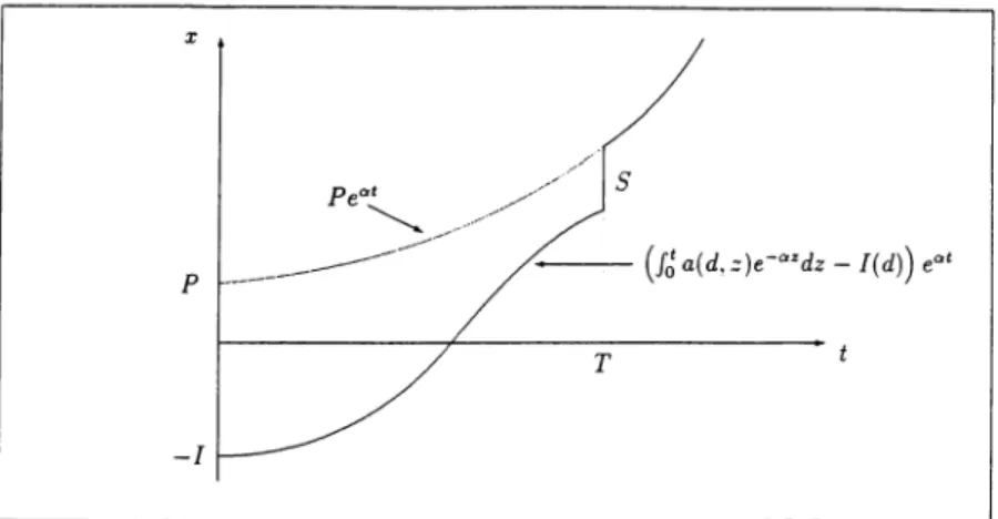
The growth model of this investment (design) situation, assuming

a

(t) =

a

(constant) is

x-{ (f~a(d,z)e-~dz-I(d))

- (f:

a(d,z)e-~dz-I(d)+S(d,1)e-aT)eat

Figure 2 illustrates such a growth process. Here,

fort< T fort~ T

(14)

represents the growth for t<T, i.e., before abandoning the system, therefore it does not include S(d,T). On the other hand, the second line of (14) represents the growth after scrapping the system, i.e., fort;;? T. After time T, only pure repro-ductive growth process of the capital generated by the system takes place.

X

T

-I

12 THE ENGINEERING EcoNOMIST • FAIL 1995 • VOLUME 41, No. 1 Also note that

therefore,

fort~ T.

Equation (14) assumes, as a typical single project invesbnent situation, two discrete cash flows, a) initial invesbnent, -I(d), at time t = 0, and b) salvage val-ue, S(d,T), at t = T. By a little more generalization, we may take into account many other discrete cash flows, a; (d) at t;. In this case, it can be shown that the solution of differential equation (1) becomes:

x

=

[I~

a(d,z')e-w.dz+

7

a;(d)e-a11 _{-I(d)+ S(d,T)e-ar}

}at

₍₁₅₎

fort~ T.

For a fixed H ~T. two measures of worth are readily determined as follows.

A=

p(

a_aJI)·

1-e

If the abandonment time Tis predetermined, an optimal invesbnent decision is found by,

max P or max A

d d

which are equivalent.

One may want to determine T optimally as well as d. In that case, it is logical to take H=T. The optimal invesbnent then is determined by,

maxP d,T maxA=max

1

a

)

. d,T d,T 1-e-ar (16) (17)

THE ENGINEERING ECONOMIST• FALL 1995 • VOLUME 41, NO. I 13 In this case, as it is seen from the models, optimal solutions from (16) and (17) are different

Next, we demonstrate that this simplest prototype model can be used for some practical and useful results on an example problem in the petroleum indus-try. This example is a simplified version of what is reported in [1].

EXAMPLE (WELL SPACING PROBLEM)

Briefly, the well spacing problem is to determine the optimal number of oil wells that should be drilled in a newly discovered petroleum reservoir (field). The term spacing refers to the portion y of the reservoir area allocated to a well. Here, the primary decision variable is the design parameter y. As the natural sequel, the abandonment time T needs to be considered as the second decision variable. Thus, to construct the model, we define:

y = number of acres (of the reservoir area) allocated to a well, T

=

time when the reservoir is abandoned (stops producing oil), R = amount of recoverable oil per unit area (acre) of the reservoir, Y = total area of the reservoir in acres,

q0 = production (flow) rate of a well at time t = 0 (the rate observed at the test well), BbVday, I

=

initial investment per well,

p

=

sale price of oil, $/Bbl,

m = rate of operating cost of a well, $/day. Assumptions:

1. The reservoir is homogeneous; i.e., R and q0 are uniform over the reser-voir area

2. Both p and m remain constant over time.

3. Oil produced from the reservoir can be sold without limit

Ifwe let:

q(y,t) = production rate of the well as a function of y and time t, and a(d,t)

=

pq(y,t)-m,

14 THE ENGINEERING ECONOMIST• FALL 1995 • VOLUME 41, No. 1

area (acre) is:

I:

£pq(y,

r>-

mie-"'

dt -1

P(y,1)= .

y (18)

It is assumed here that S(T) = 0 at the time of abandonment T. If we accept the present value as our measure of worth,

max P(y,T)

y,T

(19) detennines optimal spacing y* as well as optimal abandonment time T*. In order

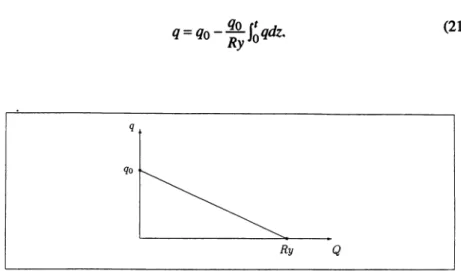
to make (19) operational, we have to obtain the functional fonn of q(y,t). For this purpose, we use the property of the behavior of petroleum reservoirs ob-tained through reservoir engineering studies, which tell us that the production rate is monotone decreasing with cumulative production Q and. for some types (solution gas drive) of reservoirs, a linear decline is a good fit as given in Figure 3. This linear decline with cumulative production, Q, leads to an exponential decline with time t, q

=

q0e-li as derived below.

Hence, the production rate q can be expressed as a linear function of Q,

q=qo- Qo _{Ry .} Q (20)

Substituting Q

=

L'

qdz in (20), we obtain the following simple integral

equa-tion: 0

(21)

Ry Q

FIGURE 3. Approximation of the production rate, q, as a linear decline of cumulative production, Q.

THE ENGINEERING ECONOMIST• FALL 1995 • VOLUME 41, No. 1 15 Solution to (21) gives:

(22) where

r

=

qo IR. This is the decay function mentioned above with 8

=

qo I Ry. Substitution of (22) in (18) yields:

(23)

An optimal solution defined in (19) then can be obtained sequentially by utilizing (23), as follows:

max P(y,

n

=

max(max P(y,

n) .

y,t y t

It can be shown that P(y, T) is concave in T and quasi-concave in y. Thus, differ-entiating (23) with respect to T and equating to zero gives,

T*

= :

In(

P!o )

=

Dy (24)

to maximize P(y,T) over T, where

D=In(P!o

),r,

Let Po(Y)

=

maxr P(y,

n.

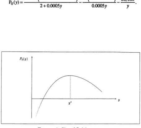
By substituting (24) in (23) for T and integrating, we get:

In order to obtain y * now,

maxP0(y)

y

must be solved. This can be done most easily by plotting Pfl.y) over y, as illus-trated in Figure 4.

Hence, the numerical value of

r

can be obtained as

r=

Dy•. It is easy to see from (25) that P<J.y) tends to - oo as y goes to zero, which can be visualized intuitively as well. It is also obvious that the total area Y of the reservoir con-stitutes an upper bound for y. Furthermore, the optimum number of wells is

16 THE ENGINEFRING EcoNOMIST • FALL 1995 • VOLUME 41, NO. 1 given roughly by Y/y*, truncated to the closest integer. (Or, it can be precisely determined by evaluating P<f.y ) for the smallest and largest integer of Y/y*.)

Let us illustrate the method by a numerical example. Suppose:

q0

=

3,000 BbVday R = 1,500 BbVacre Y = 18,000 acres I= $80,000

p

=

$20/Bbl m

=

$40/weWday

y = 3, 000/1, 500 = 2 D = In(60, 000/40/2 = 3.66

a= 0.0005$/$/day = 0.0005x365 = 0.1825 = 18.25% per year Substituting these values, equation (25) becomes:

60,ooo(1-e-3.66(2+0.000Sy>) 40(1-e-<>.OOIB3y) 80,000

Po(Y)= 2+0.0005y 0.0005y y

Po(y)

I

_y

I

y•

'DIE ENGINEERING ECONOMIST• FALL 1995 • VOLUME 41, No. 1 17

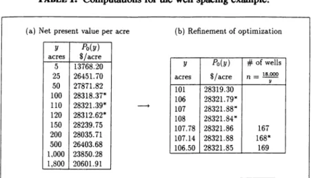
We now tabulate and plot P<fy) over y (fable l, Figure 5). Optimal values

are

found as follows. y* = 107.14 acres

n* = 168 wells

T*

=

3.66 x 107.14

=

392.1 days

max

Pr/.

y) = $28,321.88

Total net present value= 18,000 x 28, 321.88 = $509,793,840.

OTHER MEASURES OF WORTH

In the previous sections, we redefined traditionally established measures of worth and discussed associated optimization criteria with the proposed approach. These measures are quite suitable for handling a variety of problems. There are, however, many other simations where they are inadequate for arriving at good solutions. In this section, we show that it is possible to derive other measures to

suit the particularities of various problem situations by using the concept of "equivalent growth."

While the equivalent growth concept plays a crucial role in our approach, it is not new. It is the same as the concept of "equivalence of cash flows," dis-cussed in any standard engineering economy book (see, for example, [12, Chap-ter 2]). Its power, however, has not been fully exploited. Below, we discuss its versatility and illusttate our approach with an example from equipment replace-ment.

One typical and simple situation where none of the measures defined before can be used is the case where the production rate a(d,t) is not established opera-tionally; i.e., the functional form of a(d,t) cannot be determined. More specifical-ly, in most practical situations, a(d,t) being the difference between cash inflow (revenue) rate, r ( d t), and cash outflow (expense) rate, m(d,t), is:

a(d, t) = r(d, t)-m(d, t).

In many cases, m(d,t) can be determined, but r(d,t) cannot. In that case, if r(d,t)

is assumed independent of the decision variables (alternatives) d, then minimization of the present value of costs, Pc, or annual worth of costs Ac are used. This has been a common criterion in the literablre, and is very well known. If abandonment time T is a decision variable, this approach may not work as exemplified below.

Now consider a situation where:

1. manufacturing rate, q(d,t), for the products (services) produced by the system can be determined, but the sales price is unknown, or not mean-ingful (as in garbage collection, for example), and

18 'DIE ENGINEERING ECONOMIST• FALL 1995 • VOLUME 41, No. 1 2. it is assumed that all of q(d,t) are sold (utilized).

In this case, neither min Pc nor min Ac is appropriate, since the present value of revenues (benefits) is not independent of d and time t. To resolve this difficulty, we ask for what price the revenues will pay all cash outlays. Let this price be c. Hence, the equivalence between the growth of revenues and the growth of expenses gives:

(26) Solving (26) for c yields:

J:

m(d,t)e-"' dt + l(d)-S(d, T)e-ar

c--"---...---~

_-

_J:

q(d,t>e-"'t1t

(27)

Here, c can be termed as the time averaged unit cost, since the present value of

cq ( d,t) over the life T of the system is equal to the present value of the operat-ing expenses, m(d,t), plus investment outlay, l(d), minus the salvage value, S(d,T). Then, the optimi7.ation criterion is:

mine. d,T

A good example for the application of this measure is the determination of the economic life of equipment with decreasing productivity but increasing oper-ating expenses with age. Traditionally, supposing any equipment would be re-placed repeatedly with identical equipment in the future, the economic life is obtained as the solution to the following surrogate problem [4, 18):

min(J~ m(t)e-"' dt - I+ S(T)e-ar \( a_ar ).

T

\1-e

(28)

A tacit assumption is made in this approach: operating expense rate m(t) is monotone increasing with age but productivity remains the same. If productivi-ty deteriorates, (28) is not valid. This situation has been experienced in a research project involving garbage trucks ([7], see also [3]}, where:

1. operating expense rate increased exponentially with age, and

2. availability (consequently productivity) of a truck, as it gets older, de-cayed due to more frequent breakdowns and higher percentage of down time for repair with aging.

nm

ENGINEERING ECONOMIST• FALL 1995 • VOLUME 41, No. 1

TABLE 1. Computations for the well spacing example.

(a) Net present value per acre

y acres 5 25 50 100 110 120 150 200 500 1,000 1,800 $29,000 $28,000 $27,000 $26,000 Po(Y) $25,000 $24,000 $23,000 $22,000 $21,000 Po(y) $/acre 13768.20 26451.70 27871.82 28318.37* 28321.39* --+ 28312.62* 28239.75 28035. il 26403.68 23850.28 20601.91 ,,. ~

I

-... _{1---...._} (b) Refinement of optimization y Po(Y) # of wells acres $/acre n

=

1s.ooo _~ 101 28319.30 106 28321.79· 107 28321.88* 108 28321.84· 107.78 28321.86 167 107.14 28321.88 168* 106.50 28321.85 169 j

I

--... "-. !

r---,...._

I

r--

_{...._} I I 0 l 00 200 300 400 500 600 700 800 900 1,000 y (acres)

FIGURE 5. Plot of Po ( y) over y for the well spacing example.

20 llIEENGINEERINGECONOMIST•FAIL 1995• VOLUME41,NO. l

In that research, the only decision variable considered was the abandonment time (replacement age), T. All other decisions such as size, technology, and

make of the vehicle were assumed a priori made or imposed. In this case, in order to talce into account all peculiarities of the problem situation, we developed a measure, g, defined as the time averaged cost per unit quantity of service provided (per truck load of garbage collected and disposed). Derivation of the functional form of g as a function of Tis summarized below.

Let

v = truck availability index, defmed as the fraction of time that the truck is available for service,

f

=

fuel cost required for collecting and disposing a unit load of garbage,

r

=

repair and maintenance cost of a truck per year,

l = labor cost for operating a truck per year (assumed independent of truck availability),

K = total number of trips that a truck can make annually with 100% availability,

I = purchase cost of a truck, and

S = salvage value of a truck when replaced.

From the above notation, it is readily seen that

m=fvK+l+r,

where the first term is the fuel cost, the second term is the labor cost, and the third term is the repair and maintenance cost per year. Thus, the present value of expenditures over the truck's life (until it is replaced) is:

(29) Consider now the time averaged cost per unit load ofgarbage collected and disposed, g. Then, annual cost can be expressed as g K v. The present value of

all annual cash flows can be simply given as:

(30) Using the concept of equivalent growth, C must be equal to C'. Thus, equating (29) to (30) and solving for g~ we obtain:

J:

(/vK + l + r)e-at dt I - Se-di'

g= +~=-~~

nm

ENGINEERING ECONOMIST• FALL 1995 • VOLUME 41. No. 1 21 Here, the first term is the share of the operating cost and the second term is the share of the capital (amortization) costing. Thus, these terms can be called the time averaged operating cost and the time averaged capital cost per truck load of garbage.

Data analyses showed that/ and l are practically constant, but v decreases and r increases with the truck's age. More precisely, v and r have the following functional forms:

v=v0e-~. (32)

(33) for

p,

r

> 0. Substituting (32) and (33) in (31), and assuming S = 0, we obtain

the following form:

l

(l -at)

ro (

<r-a)T

l)

- -e + - - e

-I a r-a 1(/J+a

g= + _{~K(1-e-<fJ+a>T)} + _{voK 1-e-<a+fJ)T '} ( )' (34)

P+a

Hence, the solution to the replacement problem becomes: ming

T

where g is defined by equation (34).

As it is seen in this example, this particular replacement problem could not

be solved appropriately by minimizing the annual worth of cost, but only by minimizing the measure given in (34).

ExAMPLE. The following parameters were estimated for a particular truck. All monetary figures used are in 19851Ls (Turkish Lira).

v(t)

=

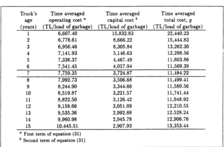
0.95e-0.09t r(t) = 126, 325e0·27' /(t) = 3,376 1L/trip l(t) = 2 M 1L/year a=10% /=10M1L K = 2 trips/day x 365 = 730 trips/year

22 'DIEENGINEFJUNGEcoNOMIST•FALL 1995• VOLUMB41,No. l TABLE 2. Computations for the truck replacement example.

Truck's Time averaged Time averaged Time averaged age operating cost • capital cost 6 _{total cost,} g

(years) (TL/load of garbage) (TL/load of garbage) (TL/load of garbage)

1 6,607.40 15,832.83 22,440.23 2 6,778.61 8,666.22 15,444.83 3 6,956.46 6,305.84 13.262.30 4 7,141.93 5,146.63 12.288.56 5 7,336.37 4,467.49 11.803.86 6 7,541.45 4,027.94 11,569.39 7 7,759.35 3,724.87 11,484.22 8 7,992.73 3,506.68 11,499.41 9 8,244.90 3,344.66 11,589.56 10 8,519.87 3,221.57 11,741.44 11 8,822.50 3,126.42 11,948.92 12 9,158.66 3,051.89 12,210.55 13 9,535.36 2,992.88 12.528.24 14 9,960.98 2,945.78 12,906.iG· 15 10.445.51 2,907.93 13,353.44

• First term of equation (31)

b Second term of equation (31)

As the trucks replaced are donated to smaller municipalities, salvage values are considered zero. Substituting all model parameters, one can solve (34) by simply tabulating g for varying values of T. Since g is a convex function of T,

the minimum g identifies the optimal replacement age, T. The computations are shown in Table 2. The optimal replacement age for this particular truck is seven years.

CONCLUSIONS AND ExTENSIONS

In this paper, we introduce a point of view that investments are growth pro-cesses, or more explicitly, investments are for growth. Interestingly, this reem-phasis of the basic purpose and goal of investment opens up another avenue for the mathematical modeling of investment decision situations. In addition, it provides another insight into understanding the nature of investment economic analysis, especially for newcomers to the field. The simple basic mathematical growth model developed here can be viewed as a unifying instrument for deriving

all traditional as well as new measures of worth. In that respect, we believe that equations (1) and (2), and their solutions (4) and (7) deserve the label the funda-mental equations of financial analysis.

The conceptualization of the set of decision (investment) alternatives as the Cartesian product, f? = D 1 x D2 x D 3 ... , in modeling opens up a possibility to

cover as many design parameters of the system as deemed appropriate, and en-ables one to conceive the investment decision process as a system design

pro-'DIE ENGINEERING ECONOMIST• FALL 1995 • VOLUME 41, No. 1 23

cess. This viewpoint brings in an additional dimension, a proper economic

anal-ysis, into the design process, which is usually overlooked.

We also bring into focus the potential use of a well known concept, cash

flow equivalence, to derive new measures of worth when the traditional measures are not suitable or convenient. In particular, we exploited the idea of time averag-ing within the context of equipment replacement. This idea can be generalized as follows. Let:

w

=

time averaged unit measure, and

a(w,t) - production rate as a function of w and time.

From equivalence, solving the following equation for w yields the measure to be

optimized:

J~

a(w,t)e-atdt

=

P(a,n

Other interesting and useful measures can be developed. A few proposals are

as follows.

1. Time averaged unit profit, profit 1t per unit quantity of product (or service) produced and sold equivalent to the net present value, can be

computed as:

P(a,n

2. Time averaged unit revenue can also be expressed similarly.

3. Profitability ratio: the ratio of the measure in item (1) into the time averaged unit cost by equation (27). This ratio can possibly be used instead of the internal rate of return.

ACKNOWLEDGMENTS

This research was supported in part by the National Science Foundation, grant DDM-9202849.

REFERENCES

[l] Aronofsky, J. S., H. Dogrusoz, and R. C. Reinitz, "Optimal Development of Under-ground Petroleum Reservoirs-Part I," Proceedings of the 4th Interna-tional Conference on OperaInterna-tional Research, 1966.

24 llIEENGINEERINGEcoNOMIST•FALL 1995• VOLUME41,N0.1 [2] Bernard, R. H., "A Comprehensive Comparison and Critique of Discounting Indices Proposed for Capital Investment Evaluation," The Engineering Econo-mist, Vol. 16, No. 3 (1971), 157-186.

[3] Bernard, R. H., "Improving the Economic Logic Underlying Replacement Age Decisions for Municipal Garbage Trucks: Case Study," The Engineering Econ-omist, Vol. 35, No. 2 (1990), 129-147.

[ 4] Bowman, E. H. and R. B. Fetter, Analysis for Production Management, Irwin,

1957.

[5] ~realey, R. A. and S. C. Myers, Principles of Corporale Finance, 3rd Edition,

McGraw-Hill, 1988.

[6] Brigham E. F., Fundamentals of Financial Management, 6th ed., The Dreyden

Press, 1992.

[7] Dogrusoz, H., N. Karabakal, and M. Denizel, "Replacement of Garbage Collec-tion Trucks with DeterioraCollec-tion in Cost and Availability," Technical Report, Systems Sciences Research Center, Middle East Technical University, Anka-ra, Turkey,. 1988.

[8] Fama, E. F. and M. H. Miller, The Theory of Finance, The Dryden Press,

Hinsdale, Illinois, 1977.

[9] Fish, J. C. L., Engineering Economics, 2nd ed., McGraw Hill, New York,

1923.

[10] Fisher, I., The Theory of Interest, New York, Augustus M. Kelley Publishers,

1965. Reprinted from the 1930 edition.

[11] Grant, E. L., Principles of Engineering Economy, New York, 1930.

[12] Grant, E. L., W. G. Ireson, and R. S. Leavenworth, Principles of Engineering Economy, Eighth edition, Wiley, 1990.

[13] Hirshleifer, J., "On the Theory of Optimal Investment Decision," Journal of Political Economy, (1958).

[14] Lohmann, J. R., "The IRR, NPV and the Fallacy of the Reinvestment Rate Assumptions," The Engineering Economist, Vol. 33, No. 4 (1988), 303-330.

[15] Oakford, R. V., S. A. Bhimjee, and J. V. Jucker, "The Internal Rate of Return, the Pseudo Internal Rate of Return, and the NPV and Their Use in Financial Decision Making," The Engineering Economist, Vol. 22, No. 3 (1977),

187-201.

[16] Park, C. S. and G. P. Sharp-Bette, Advanced Engineering Economics, Wiley,

1990.

[17] Simon, H. A., Models of Man, New York, Wiley, 1957.

[18] Terborgh, G., Dynamic Equipment Policy, Machinery and Allied Products

Institute, Washington D.C., 1949.

[19] Weingartner, H. M., "Some New Views on the Payback Period and Capital Budgeting Decision," Management Science, Vol. 15, No. 12 (1969),

THE ENGINEERING EcoNOMIST • FALL 1995 • VOLUME 41, No. 1 25

BIOGRAPHICAL SKETCHES

HALIM Dooausoz is Professor of Industrial Engineering at Bilkent University,

Tur-key. He received his B.S. and M.S. in Mechanical Engineering from Istanbul Techni-cal University, Turkey, and his Ph.D. In Operations Research from Case Institute of Technology. His research interests include the methodology of decision modeling, investment decision making, and financial analysis. Professor Dogrusoz has exten-sive experience in applied research. Previously, he has taught at Brooklyn Polytech-nic Institute, Stevens Institute of Technology, Middle East TechPolytech-nical University (Turkey), University of Pennsylvania, and North Carolina State University.

NEJAT KARABAKAL is Visiting Assistant Professor at the University of Michigan. Previously, he taught at Bilkent University, Turkey. He received his B.S. and M.S. in industrial engineering from Middle East Technical University, Turkey, and his Ph.D. in Industrial and Operations Engineering from the University of Michigan. His re-search interests include equipment replacement and integer programming.