Fast Stiffness Matrix Calculation for Nonlinear Finite Element Method

(1)

Research Article

Fast Stiffness Matrix Calculation for Nonlinear

Finite Element Method

Emir Gülümser,

1

U

Lur Güdükbay,

1

and Sinan Filiz

2

1_{Department of Computer Engineering, Bilkent University, 06800 Ankara, Turkey} 2_{Department of Mechanical Engineering, Bilkent University, 06800 Ankara, Turkey}

Correspondence should be addressed to U˘gur G¨ud¨ukbay; gudukbay@cs.bilkent.edu.tr Received 29 May 2014; Revised 24 July 2014; Accepted 6 August 2014; Published 28 August 2014 Academic Editor: Henggui Zhang

Copyright © 2014 Emir G¨ul¨umser et al. This is an open access article distributed under the Creative Commons Attribution License, which permits unrestricted use, distribution, and reproduction in any medium, provided the original work is properly cited. We propose a fast stiffness matrix calculation technique for nonlinear finite element method (FEM). Nonlinear stiffness matrices are constructed using Green-Lagrange strains, which are derived from infinitesimal strains by adding the nonlinear terms discarded from small deformations. We implemented a linear and a nonlinear finite element method with the same material properties to examine the differences between them. We verified our nonlinear formulation with different applications and achieved considerable speedups in solving the system of equations using our nonlinear FEM compared to a state-of-the-art nonlinear FEM.

1. Introduction

Mesh deformations have widespread usage areas, such as computer games, computer animations, fluid flow, heat transfer, surgical simulations, cloth simulations, and crash test simulations. The major goal in mesh deformations is to establish a good balance between the accuracy of the simulation and the computational cost; achieving this balance depends on the application. The speed of the simulation is far more important than the accuracy in computer games. The simulation needs to be real-time in order to be used in games so free-form deformation or fast linear FEM solvers can be used. However, high computation cost gives much more accurate results when we are working with life-critical applications such as car crash tests, surgical simulators, and concrete analysis of buildings; even linear FEM solvers are not adequate enough for these types of applications in terms of the accuracy.

For realistic and highly accurate deformations, one can use the finite element method (FEM), a numerical technique to find approximate solutions to engineering and mathemat-ical physics problems. FEM could be used to solve problems

in areas such as structural analysis, heat transfer, fluid flow, mass transport, and electromagnetics [1,2].

We propose a fast stiffness matrix calculation technique for nonlinear FEM. We derive nonlinear stiffness matri-ces using Green-Lagrange strains, themselves derived from infinitesimal strains by adding the nonlinear terms discarded from infinitesimal strain theory.

We mainly focus on the construction of the stiffness matrices because change in material parameters and change in boundary conditions can be directly represented and applied without choosing a proper FEM [3]. Joldes et al. [4] and Taylor et al. [5] achieve real-time computations of soft tissue deformations for nonlinear FEM using GPUs; however, they do not describe how they compute stiffness matrices; thus, we cannot implement their methods and compare them with our proposed method. Cerrolaza and Osorio describe a simple and efficient method to reduce the integration time of nonlinear FEM for dynamic problems using hexahedral 8-noded finite elements [6]. We compare our stiffness matrix calculations with Pedersen’s method [3] to measure performance and verify correctness. We achieve a 142% speedup in calculating the stiffness matrices and a 15%

Volume 2014, Article ID 932314, 12 pages http://dx.doi.org/10.1155/2014/932314

(2)

speedup in solving the whole system on average, compared to Pedersen’s method.

2. The Nonlinear FEM with

Green-Lagrange Strains

We use tetrahedral elements for modeling meshes in the experiments. Overall, there are 12 unknown nodal displace-ments in a tetrahedral element. They are given by [2]

{𝑑} = {𝑢 (𝑥, 𝑦, 𝑧)} = { { { { { { { { { { { { { { { { { { { { { 𝑢₁ V1 𝑤1 .. . 𝑢₄ V₄ 𝑤₄ } } } } } } } } } } } } } } } } } } } } } . (1)

In global coordinates, we represent displacements by linear function by

𝑢𝑒(𝑥, 𝑦, 𝑧) = 𝑐₁+ 𝑐₂𝑥 + 𝑐₃𝑦 + 𝑐₄𝑧. (2) For all 4 vertices, (2) is extended as

[ [ [ [ 1 𝑥₁ 𝑦₁ 𝑧₁ 1 𝑥₂ 𝑦₂ 𝑧₂ 1 𝑥₃ 𝑦₃ 𝑧₃ 1 𝑥₄ 𝑦₄ 𝑧₄ ] ] ] ] { { { { { { { 𝑐₁ 𝑐₂ 𝑐₃ 𝑐₄ } } } } } } } = { { { { { { { 𝑢₁ 𝑢₂ 𝑢₃ 𝑢₄ } } } } } } } . (3)

Constants𝑐_𝑛can be found as

𝑐_𝑛= V−1𝑢_𝑛, (4) whereV−1is given by V−1= 1 det(V) [ [ [ [ 𝛼₁ 𝛼₂ 𝛼₃ 𝛼₄ 𝛽₁ 𝛽₂ 𝛽₃ 𝛽₄ 𝛾₁ 𝛾₂ 𝛾₃ 𝛾₄ 𝛿₁ 𝛿₂ 𝛿₃ 𝛿₄ ] ] ] ] . (5)

det(V) is 6𝑉, where 𝑉 is the volume of the tetrahedron. If we substitute (4) into (2), we obtain

𝑢𝑒(𝑥, 𝑦, 𝑧) =_6𝑉1_𝑒[1 𝑥 𝑦 𝑧][[_[ [ 𝛼₁ 𝛼₂ 𝛼₃ 𝛼₄ 𝛽₁ 𝛽₂ 𝛽₃ 𝛽₄ 𝛾₁ 𝛾₂ 𝛾₃ 𝛾₄ 𝛿₁ 𝛿₂ 𝛿₃ 𝛿₄ ] ] ] ] { { { { { { { 𝑢₁ 𝑢₂ 𝑢₃ 𝑢₄ } } } } } } } . (6)

𝛼, 𝛽, 𝛾, 𝛿, and the volume 𝑉 are calculated by 𝛼₁=󵄨󵄨󵄨󵄨󵄨󵄨󵄨󵄨 󵄨󵄨󵄨󵄨 𝑥₂ 𝑦₂ 𝑧₂ 𝑥₃ 𝑦₃ 𝑧₃ 𝑥₄ 𝑦₄ 𝑧₄ 󵄨󵄨󵄨󵄨 󵄨󵄨󵄨󵄨 󵄨󵄨󵄨󵄨, 𝛼2= −󵄨󵄨󵄨󵄨󵄨󵄨󵄨󵄨 󵄨󵄨󵄨󵄨 𝑥₁ 𝑦₁ 𝑧₁ 𝑥₃ 𝑦₃ 𝑧₃ 𝑥₄ 𝑦₄ 𝑧₄ 󵄨󵄨󵄨󵄨 󵄨󵄨󵄨󵄨 󵄨󵄨󵄨󵄨, 𝛼₃=󵄨󵄨󵄨󵄨󵄨󵄨󵄨󵄨 󵄨󵄨󵄨󵄨 𝑥₁ 𝑦₁ 𝑧₁ 𝑥₂ 𝑦₂ 𝑧₂ 𝑥₄ 𝑦₄ 𝑧₄ 󵄨󵄨󵄨󵄨 󵄨󵄨󵄨󵄨 󵄨󵄨󵄨󵄨, 𝛼4= −󵄨󵄨󵄨󵄨󵄨󵄨󵄨󵄨 󵄨󵄨󵄨󵄨 𝑥₁ 𝑦₁ 𝑧₁ 𝑥₂ 𝑦₂ 𝑧₂ 𝑥₃ 𝑦₃ 𝑧₃ 󵄨󵄨󵄨󵄨 󵄨󵄨󵄨󵄨 󵄨󵄨󵄨󵄨, 𝛽₁= −󵄨󵄨󵄨󵄨󵄨󵄨󵄨󵄨 󵄨󵄨󵄨󵄨 1 𝑦₂ 𝑧₂ 1 𝑦₃ 𝑧₃ 1 𝑦₄ 𝑧₄ 󵄨󵄨󵄨󵄨 󵄨󵄨󵄨󵄨 󵄨󵄨󵄨󵄨, 𝛽2=󵄨󵄨󵄨󵄨󵄨󵄨󵄨󵄨 󵄨󵄨󵄨󵄨 1 𝑦₁ 𝑧₁ 1 𝑦₃ 𝑧₃ 1 𝑦₄ 𝑧₄ 󵄨󵄨󵄨󵄨 󵄨󵄨󵄨󵄨 󵄨󵄨󵄨󵄨, 𝛽₃= −󵄨󵄨󵄨󵄨󵄨󵄨󵄨󵄨 󵄨󵄨󵄨󵄨 1 𝑦₁ 𝑧₁ 1 𝑦2 𝑧2 1 𝑦4 𝑧4 󵄨󵄨󵄨󵄨 󵄨󵄨󵄨󵄨 󵄨󵄨󵄨󵄨, 𝛽4=󵄨󵄨󵄨󵄨󵄨󵄨󵄨󵄨 󵄨󵄨󵄨󵄨 1 𝑦₁ 𝑧₁ 1 𝑦2 𝑧2 1 𝑦3 𝑧3 󵄨󵄨󵄨󵄨 󵄨󵄨󵄨󵄨 󵄨󵄨󵄨󵄨, 𝛾1=󵄨󵄨󵄨󵄨󵄨󵄨󵄨󵄨 󵄨󵄨󵄨󵄨 1 𝑥₂ 𝑧₂ 1 𝑥₃ 𝑧₃ 1 𝑥₄ 𝑧₄ 󵄨󵄨󵄨󵄨 󵄨󵄨󵄨󵄨 󵄨󵄨󵄨󵄨, 𝛾2= −󵄨󵄨󵄨󵄨󵄨󵄨󵄨󵄨 󵄨󵄨󵄨󵄨 1 𝑥₁ 𝑧₁ 1 𝑥₃ 𝑧₃ 1 𝑥₄ 𝑧₄ 󵄨󵄨󵄨󵄨 󵄨󵄨󵄨󵄨 󵄨󵄨󵄨󵄨, 𝛾₃=󵄨󵄨󵄨󵄨󵄨󵄨󵄨󵄨 󵄨󵄨󵄨󵄨 1 𝑥₁ 𝑧₁ 1 𝑥₂ 𝑧₂ 1 𝑥₄ 𝑧₄ 󵄨󵄨󵄨󵄨 󵄨󵄨󵄨󵄨 󵄨󵄨󵄨󵄨, 𝛾4= −󵄨󵄨󵄨󵄨󵄨󵄨󵄨󵄨 󵄨󵄨󵄨󵄨 1 𝑥₁ 𝑧₁ 1 𝑥₂ 𝑧₂ 1 𝑥₃ 𝑧₃ 󵄨󵄨󵄨󵄨 󵄨󵄨󵄨󵄨 󵄨󵄨󵄨󵄨, 𝛿₁= −󵄨󵄨󵄨󵄨󵄨󵄨󵄨󵄨 󵄨󵄨󵄨󵄨 1 𝑥₂ 𝑦₂ 1 𝑥₃ 𝑦₃ 1 𝑥₄ 𝑦₄ 󵄨󵄨󵄨󵄨 󵄨󵄨󵄨󵄨 󵄨󵄨󵄨󵄨, 𝛿2=󵄨󵄨󵄨󵄨󵄨󵄨󵄨󵄨 󵄨󵄨󵄨󵄨 1 𝑥₁ 𝑦₁ 1 𝑥₃ 𝑦₃ 1 𝑥₄ 𝑦₄ 󵄨󵄨󵄨󵄨 󵄨󵄨󵄨󵄨 󵄨󵄨󵄨󵄨, 𝛿₃= −󵄨󵄨󵄨󵄨󵄨󵄨󵄨󵄨 󵄨󵄨󵄨󵄨 1 𝑥₁ 𝑦₁ 1 𝑥₂ 𝑦₂ 1 𝑥₄ 𝑦₄ 󵄨󵄨󵄨󵄨 󵄨󵄨󵄨󵄨 󵄨󵄨󵄨󵄨, 𝛿4=󵄨󵄨󵄨󵄨󵄨󵄨󵄨󵄨 󵄨󵄨󵄨󵄨 1 𝑥₁ 𝑦₁ 1 𝑥₂ 𝑦₂ 1 𝑥₃ 𝑦₃ 󵄨󵄨󵄨󵄨 󵄨󵄨󵄨󵄨 󵄨󵄨󵄨󵄨, 6𝑉 =󵄨󵄨󵄨󵄨󵄨󵄨󵄨󵄨_{󵄨󵄨󵄨󵄨} 󵄨󵄨󵄨󵄨 1 𝑥_𝑖 𝑦_𝑖 𝑧_𝑖 1 𝑥𝑗 𝑦𝑗 𝑧𝑗 1 𝑥_𝑘 𝑦_𝑘 𝑧_𝑘 1 𝑥_𝑙 𝑦_𝑙 𝑧_𝑙 󵄨󵄨󵄨󵄨 󵄨󵄨󵄨󵄨 󵄨󵄨󵄨󵄨 󵄨󵄨󵄨󵄨. (7) Because of the differentials in strain calculation,𝛼 is not used in the following stages. If we expand (6), we obtain

𝑢𝑒(𝑥, 𝑦, 𝑧) = _6𝑉1_𝑒 [[_[ [ 𝛼₁+ 𝛽₁𝑥 + 𝛾₁𝑦 + 𝛿₁𝑧 𝛼₂+ 𝛽₂𝑥 + 𝛾₂𝑦 + 𝛿₂𝑧 𝛼₃+ 𝛽₃𝑥 + 𝛾₃𝑦 + 𝛿₃𝑧 𝛼₄+ 𝛽₄𝑥 + 𝛾₄𝑦 + 𝛿₄𝑧 ] ] ] ] × [𝑢(𝑥, 𝑦, 𝑧)₁ 𝑢(𝑥, 𝑦, 𝑧)₂ 𝑢(𝑥, 𝑦, 𝑧)₃ 𝑢(𝑥, 𝑦, 𝑧)₄] . (8)

For tetrahedral elements, to express displacements in simpler form, shape functions are introduced (𝜓₁, 𝜓₂, 𝜓₃, 𝜓₄). They are given by 𝜓1= _6𝑉1 (𝛼1+ 𝛽1𝑥 + 𝛾1𝑦 + 𝛿1𝑧) 𝑢(𝑥, 𝑦, 𝑧)1, 𝜓₂= 1 6𝑉(𝛼2+ 𝛽2𝑥 + 𝛾2𝑦 + 𝛿2𝑧) 𝑢(𝑥, 𝑦, 𝑧)2, 𝜓₃= 1 6𝑉(𝛼3+ 𝛽3𝑥 + 𝛾3𝑦 + 𝛿3𝑧) 𝑢(𝑥, 𝑦, 𝑧)3, 𝜓₄= _6𝑉1 (𝛼₄+ 𝛽₄𝑥 + 𝛾₄𝑦 + 𝛿₄𝑧) 𝑢(𝑥, 𝑦, 𝑧)₄. (9)

In our method, nonlinear stiffness matrices are derived using Green-Lagrange strains (large deformations), which

(3)

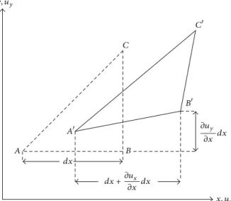
y, uy x, ux dx C C 󳰀 B B 󳰀 A A 󳰀 𝜕uy 𝜕x dx dx +𝜕ux 𝜕x dx

Figure 1: 2D element before and after deformation.

themselves are derived directly from infinitesimal strains (small deformations), by adding the nonlinear terms dis-carded in infinitesimal strain theory. The proposed nonlinear FEM uses the linear FEM framework but it does not require the explicit use of weight functions and differential equations. Hence, numerical integration is not needed for the solution of the proposed nonlinear FEM. Instead of using weight func-tions and integrals, we use displacement gradients and strains to make the elemental stiffness matrices space-independent in order to discard the integral. We extend the linear FEM to the nonlinear FEM by extending the linear strains to the Green-Lagrange strains.

We constructed our linear FEM by extending Logan’s 2D linear FEM to 3D [2]. To understand Green-Lagrange strains, we must first see how they differ from the infinitesimal strains used to calculate the global stiffness matrices in a linear FEM. Figure 1shows a 2D element before and after deformation, where the element edge𝐴𝐵 with initial length 𝑑𝑥 becomes 𝐴󸀠_𝐵󸀠_{. The engineering normal strain is calculated as the}

change in the length of the line

𝜀𝑥= 󵄨󵄨󵄨󵄨󵄨𝐴 󸀠_𝐵󸀠󵄨󵄨󵄨󵄨

󵄨 − |𝐴𝐵|

|𝐴𝐵| . (10)

The final length of the elemental edge can be calculated using 󵄨󵄨󵄨󵄨 󵄨𝐴󸀠𝐵󸀠󵄨󵄨󵄨󵄨󵄨2= (𝑑𝑥 +𝜕𝑢_𝜕𝑥𝑥𝑑𝑥) 2 + (𝜕𝑢𝑦 𝜕𝑥𝑑𝑥) 2 , 󵄨󵄨󵄨󵄨 󵄨𝐴󸀠𝐵󸀠󵄨󵄨󵄨󵄨󵄨2= 𝑑𝑥2[1 + 2 (𝜕𝑢_𝜕𝑥𝑥) + (𝜕𝑢_𝜕𝑥𝑥) 2 + (𝜕𝑢𝑦 𝜕𝑥) 2 ] . (11)

By neglecting the higher-order terms in (11), 2D infinitesimal strains are defined by

𝜀_𝑥𝑥= 𝜕𝑢_𝜕𝑥𝑥, 𝜀_𝑦𝑦= 𝜕𝑢_𝜕𝑦𝑦, 𝜀_𝑥𝑦 =1₂(𝜕𝑢_𝜕𝑦𝑥 +𝜕𝑢_𝜕𝑥𝑦) . (12)

By the definition, the nonlinear FEM differs from the linear FEM because of the nonlinearity that arises from the higher-order term neglected in calculation of strains. The strain vector used in the linear FEM relies on the assumption that the displacements at the𝑥-axis, 𝑦-axis, and 𝑧-axis are very small. The initial and final positions of a given particle are practically the same; thus, the higher-order terms are neglected [7]. When the displacements are large, however, this is no longer the case and one must distinguish between the initial and final coordinates of the particles; thus the higher-order terms are added into the strain equations. By adding these high-order terms, 3D strains are defined as [8]

𝜂_𝑥𝑥= 𝜕𝑢𝑥 𝜕𝑥 + 1 2[( 𝜕𝑢_𝑥 𝜕𝑥 𝜕𝑢_𝑥 𝜕𝑥) + ( 𝜕𝑢_𝑦 𝜕𝑥 𝜕𝑢_𝑦 𝜕𝑥) + ( 𝜕𝑢_𝑧 𝜕𝑥 𝜕𝑢_𝑧 𝜕𝑥)] , 𝜂_𝑦𝑦=𝜕𝑢𝑦 𝜕𝑦 + 1 2[( 𝜕𝑢_𝑥 𝜕𝑦 𝜕𝑢_𝑥 𝜕𝑦 ) + ( 𝜕𝑢_𝑦 𝜕𝑦 𝜕𝑢_𝑦 𝜕𝑦) + ( 𝜕𝑢_𝑧 𝜕𝑦 𝜕𝑢_𝑧 𝜕𝑦)] , 𝜂_𝑧𝑧=𝜕𝑢𝑧 𝜕𝑧 + 1 2[( 𝜕𝑢𝑥 𝜕𝑧 𝜕𝑢𝑥 𝜕𝑧 ) + ( 𝜕𝑢_𝑦 𝜕𝑧 𝜕𝑢_𝑦 𝜕𝑧) + ( 𝜕𝑢_𝑧 𝜕𝑧 𝜕𝑢_𝑧 𝜕𝑧)] , 𝜂_𝑥𝑦= 1₂(𝜕𝑢_𝜕𝑦𝑥 +𝜕𝑢_𝜕𝑥𝑦) +₂1[(𝜕𝑢_𝜕𝑥𝑥𝜕𝑢_𝜕𝑦𝑥) + (𝜕𝑢_𝜕𝑥𝑦𝜕𝑢_𝜕𝑦𝑦) + (𝜕𝑢_𝜕𝑥𝑧𝜕𝑢_𝜕𝑦𝑧)] , 𝜂_𝑧𝑥= 1 2( 𝜕𝑢_𝑧 𝜕𝑥 + 𝜕𝑢_𝑥 𝜕𝑧) +1₂[(𝜕𝑢𝑥 𝜕𝑧 𝜕𝑢_𝑥 𝜕𝑥) + ( 𝜕𝑢_𝑦 𝜕𝑧 𝜕𝑢_𝑦 𝜕𝑥) + ( 𝜕𝑢_𝑧 𝜕𝑧 𝜕𝑢_𝑧 𝜕𝑥)] , 𝜂_𝑦𝑧= 1 2( 𝜕𝑢_𝑦 𝜕𝑧 + 𝜕𝑢_𝑧 𝜕𝑦) +1 2[( 𝜕𝑢_𝑥 𝜕𝑦 𝜕𝑢_𝑥 𝜕𝑧) + ( 𝜕𝑢_𝑦 𝜕𝑦 𝜕𝑢_𝑦 𝜕𝑧 ) + ( 𝜕𝑢_𝑧 𝜕𝑦 𝜕𝑢_𝑧 𝜕𝑧)] , (13) which leads to {𝑛} = { { { { { { { { { { { { { { { { { 𝜂_𝑥𝑥 𝜂_𝑦𝑦 𝜂𝑧𝑧 2 (𝜂_𝑥𝑦+ 𝜂_𝑦𝑥) 2 (𝜂𝑥𝑧+ 𝜂𝑧𝑥) 2 (𝜂_𝑦𝑧+ 𝜂_𝑧𝑦) } } } } } } } } } } } } } } } } } = { { { { { { { { { { { { { { { 𝜂_𝑥𝑥 𝜂_𝑦𝑦 𝜂_𝑧𝑧 2𝜂_𝑥𝑦 2𝜂𝑧𝑥 2𝜂𝑦𝑧 } } } } } } } } } } } } } } } . (14)

The Green-Lagrange strain tensor is represented in matrix notation as

{𝜂} = [𝐵𝑇_𝐿] {𝑑} +1₂{𝑑}𝑇[𝐵NL] {𝑑} , (15)

where{𝑑} is the nodal displacement, [𝐵_𝐿] is the linear, and [𝐵NL] is the nonlinear part of the [𝐵0] matrix [3]. For a specific

(4)

element, [𝐵_𝐿] and[𝐵NL] are constant, as with the [𝐵] matrix

in the linear FEM. With the variation of{𝑑} [9], (15) becomes {𝜂} = [𝐵𝑇_𝐿] {𝑑} + {𝑑}𝑇[𝐵NL] {𝑑} . (16)

Gathering the strain components together, we can rewrite (15) and (16) as

{𝜂} = ([𝐵_𝐿] +1

2{𝑑𝑇} [ 𝐵NL]) {𝑑} = [ 𝐵0] {𝑑} ,

{𝜂} = ([𝐵_𝐿] + {𝑑𝑇} [ 𝐵NL]) {𝑑} = [𝐵0] {𝑑} .

(17)

The linear part of the[𝐵₀] matrix ([𝐵_𝐿]) is the same as the [𝐵] matrix in the linear FEM. Calculating [𝐵₀] becomes more complex with the introduction of the nonlinear terms. After finding the nonlinear strains, these equations are combined with the shape functions to find matrix[𝐵₀]:

{𝜂} = [𝐵₀] {𝑑} . (18)

The most frequently used terms, which are the nine dis-placement gradients for calculating the nonlinear strains, are 𝜕𝑢_𝑥/𝜕𝑥, 𝜕𝑢_𝑥/𝜕𝑦, 𝜕𝑢_𝑥/𝜕𝑧, 𝜕𝑢_𝑦/𝜕𝑥, 𝜕𝑢_𝑦/𝜕𝑦, 𝜕𝑢_𝑦/𝜕𝑥, 𝜕𝑢_𝑧/𝜕𝑥, 𝜕𝑢_𝑧/𝜕𝑦, and 𝜕𝑢_𝑧/𝜕𝑧. Using (8) for displacements, we can con-struct the displacement gradients using the partial derivatives of the shape functions. They are represented by

𝑢𝑥𝑥= _6𝑉1 (𝛽1𝑢1+ 𝛽2𝑢2+ 𝛽3𝑢3+ 𝛽4𝑢4) , 𝑢_𝑦𝑥= 1 6𝑉(𝛽1V1+ 𝛽2V2+ 𝛽3V3+ 𝛽4V4) , 𝑢_𝑧𝑥= 1 6𝑉(𝛽1𝑤1+ 𝛽2𝑤2+ 𝛽3𝑤3+ 𝛽4𝑤4) , 𝑢_𝑥𝑦= _6𝑉1 (𝛾₁𝑢₁+ 𝛾₂𝑢₂+ 𝛾₃𝑢₃+ 𝛾₄𝑢₄) , 𝑢_𝑦𝑦= 1 6𝑉(𝛾1V1+ 𝛾2V2+ 𝛾3V3+ 𝛾4V4) , 𝑢_𝑧𝑦=_6𝑉1 (𝛾₁𝑤₁+ 𝛾₂𝑤₂+ 𝛾₃𝑤₃+ 𝛾₄𝑤₄) , 𝑢_𝑥𝑧= 1 6𝑉(𝛿1𝑢1+ 𝛿2𝑢2+ 𝛿3𝑢3+ 𝛿4𝑢4) , 𝑢𝑦𝑧= _6𝑉1 (𝛿1V1+ 𝛿2V2+ 𝛿3V3+ 𝛿4V4) , 𝑢_𝑧𝑧= 1 6𝑉(𝛿1𝑤1+ 𝛿2𝑤2+ 𝛿3𝑤3+ 𝛿4𝑤4) , (19) where𝑢_𝑥𝑥represents𝜕𝑢_𝑥/𝜕𝑥.

We can evaluate the partial derivatives of the shape functions as follows (for the 1st node of[𝐵NL]):

[(𝜕𝑢𝑥 𝜕𝑥 𝜕𝑢_𝑥 𝜕𝑥) + ( 𝜕𝑢_𝑦 𝜕𝑥 𝜕𝑢_𝑦 𝜕𝑥) + ( 𝜕𝑢_𝑧 𝜕𝑥 𝜕𝑢_𝑧 𝜕𝑥)] = 1 6𝑉(𝛽1(𝑢𝑥𝑥+ 𝑢𝑦𝑥+ 𝑢𝑧𝑥)) , [(𝜕𝑢𝑥 𝜕𝑦 𝜕𝑢_𝑥 𝜕𝑦 ) + ( 𝜕𝑢_𝑦 𝜕𝑦 𝜕𝑢_𝑦 𝜕𝑦) + ( 𝜕𝑢𝑧 𝜕𝑦 𝜕𝑢𝑧 𝜕𝑦)] = _6𝑉1 (𝛾₁(𝑢_𝑥𝑦+ 𝑢_𝑦𝑦+ 𝑢_𝑧𝑦)) , [(𝜕𝑢𝑥 𝜕𝑧 𝜕𝑢_𝑥 𝜕𝑧 ) + ( 𝜕𝑢𝑦 𝜕𝑧 𝜕𝑢𝑦 𝜕𝑧) + ( 𝜕𝑢_𝑧 𝜕𝑧 𝜕𝑢_𝑧 𝜕𝑧)] = 1 6𝑉(𝛿1(𝑢𝑥𝑧+ 𝑢𝑦𝑧+ 𝑢𝑧𝑧)) , [(𝜕𝑢𝑥 𝜕𝑥 𝜕𝑢_𝑥 𝜕𝑦 ) + ( 𝜕𝑢_𝑦 𝜕𝑥 𝜕𝑢_𝑦 𝜕𝑦) + ( 𝜕𝑢_𝑧 𝜕𝑥 𝜕𝑢_𝑧 𝜕𝑦)] = _6𝑉1 (𝛾1(𝑢𝑥𝑥+ 𝑢𝑦𝑥+ 𝑢𝑧𝑥)) +_6𝑉1 (𝛽₁(𝑢_𝑥𝑦+ 𝑢_𝑦𝑦+ 𝑢_𝑧𝑦)) , [(𝜕𝑢𝑥 𝜕𝑧 𝜕𝑢_𝑥 𝜕𝑥) + ( 𝜕𝑢𝑦 𝜕𝑧 𝜕𝑢𝑦 𝜕𝑥) + ( 𝜕𝑢_𝑧 𝜕𝑧 𝜕𝑢_𝑧 𝜕𝑥)] = 1 6𝑉(𝛿1(𝑢𝑥𝑥+ 𝑢𝑦𝑥+ 𝑢𝑧𝑥)) +_6𝑉1 (𝛽1(𝑢𝑥𝑧+ 𝑢𝑦𝑧+ 𝑢𝑧𝑧)) , [(𝜕𝑢𝑥 𝜕𝑦 𝜕𝑢_𝑥 𝜕𝑧 ) + ( 𝜕𝑢_𝑦 𝜕𝑦 𝜕𝑢_𝑦 𝜕𝑧) + ( 𝜕𝑢_𝑧 𝜕𝑦 𝜕𝑢_𝑧 𝜕𝑧)] = _6𝑉1 (𝛾1(𝑢𝑥𝑧+ 𝑢𝑦𝑧+ 𝑢𝑧𝑧)) + 1 6𝑉(𝛿1(𝑢𝑥𝑦+ 𝑢𝑦𝑦+ 𝑢𝑧𝑦)) . (20) Using (17) and (20), we obtain [𝐵₀] for the 1st node (21). Similarly, using (17) and (20), we obtain[𝐵₀] for the 1st node (22).

(5)

Consider [𝐵₀₁] = [ [ [ [ [ [ [ [ [ [ [ [ [ [ [ 𝛽₁+ 𝛽₁(𝑢_𝑥𝑥) 𝛽₁(𝑢_𝑦𝑥) 𝛽₁(𝑢_𝑧𝑥) 𝛾1(𝑢𝑥𝑦) 𝛾1+ 𝛾1(𝑢𝑦𝑦) 𝛾1(𝑢𝑧𝑦) 𝛿₁(𝑢_𝑥𝑧) 𝛿₁(𝑢_𝑦𝑧) 𝛿₁+ 𝛿₁(𝑢_𝑧𝑧) 𝛾₁+ 𝛾₁(𝑢_𝑥𝑥) + 𝛽₁(𝑢_𝑥𝑦) 𝛾₁(𝑢_𝑦𝑥) + 𝛽₁+ 𝛽₁(𝑢_𝑦𝑦) 𝛾₁(𝑢_𝑧𝑥) + 𝛽₁(𝑢_𝑧𝑦) 𝛿1+ 𝛿1(𝑢𝑥𝑥) + 𝛽1(𝑢𝑥𝑧) 𝛿1(𝑢𝑦𝑥) + 𝛽1(𝑢𝑦𝑧) 𝛿1(𝑢𝑧𝑥) + 𝛽1+ 𝛽1(𝑢𝑧𝑧) 𝛾₁(𝑢_𝑥𝑧) + 𝛿₁(𝑢_𝑥𝑦) 𝛾₁+ 𝛾₁(𝑢_𝑦𝑧) + 𝛿₁(𝑢_𝑦𝑦) 𝛾₁(𝑢_𝑧𝑧) + 𝛿₁+ 𝛿₁(𝑢_𝑧𝑦) ] ] ] ] ] ] ] ] ] ] ] ] ] ] ] { { { 𝑢1 V₁ 𝑤₁ } } } , (21) [𝐵₀₁] = [ [ [ [ [ [ [ [ [ [ [ [ [ [ [ [ [ [ [ [ [ [ 𝛽₁+1₂𝛽₁(𝑢_𝑥𝑥) 1₂𝛽₁(𝑢_𝑦𝑥) 1₂𝛽₁(𝑢_𝑧𝑥) 1 2𝛾1(𝑢𝑥𝑦) 𝛾1+ 1 2𝛾1(𝑢𝑦𝑦) 1 2𝛾1(𝑢𝑧𝑦) 1 2𝛿1(𝑢𝑥𝑧) 1₂𝛿1(𝑢𝑦𝑧) 𝛿1+1₂𝛿1(𝑢𝑧𝑧) 𝛾₁+1 2𝛾1(𝑢𝑥𝑥) + 1 2𝛽1(𝑢𝑥𝑦) 1 2𝛾1(𝑢𝑦𝑥) + 𝛽1+ 1 2𝛽1(𝑢𝑦𝑦) 1 2𝛾1(𝑢𝑧𝑥) + 1 2𝛽1(𝑢𝑧𝑦) 𝛿₁+1 2𝛿1(𝑢𝑥𝑥) + 1 2𝛽1(𝑢𝑥𝑧) 1 2𝛿1(𝑢𝑦𝑥) + 1 2𝛽1(𝑢𝑦𝑧) 1 2𝛿1(𝑢𝑧𝑥) + 𝛽1+ 1 2𝛽1(𝑢𝑧𝑧) 1 2𝛾1(𝑢𝑥𝑧) +1₂𝛿1(𝑢𝑥𝑦) 𝛾1+1₂𝛾1(𝑢𝑦𝑧) +1₂𝛿1(𝑢𝑦𝑦) 1₂𝛾1(𝑢𝑧𝑧) + 𝛿1+1₂𝛿1(𝑢𝑧𝑦) ] ] ] ] ] ] ] ] ] ] ] ] ] ] ] ] ] ] ] ] ] ] { { { 𝑢₁ V₁ 𝑤₁ } } } . (22)

The FEM is derived from conservation of the potential energy, which is defined by

𝜋 = Estrain+ 𝑊, (23)

where Estrainis the strain energy of the linear element and𝑊

is the work potential. They are given by

Estrain= 1₂∫ Ω𝑒𝜀

𝑇_{𝜎𝑑𝑥,} _{𝑊 = 𝑓}𝑒_𝑑𝑇_, ₍₂₄₎

where the engineering strain vector{𝜀} is

{𝜀} = [𝐵] {𝑑} . (25)

From (24), the engineering stress vector𝜏 is related to the strain vector by

𝜏 = [𝐸] {𝜂} = [𝐸] [𝐵0] {𝑑} . (26)

The secant relations are described by the matrix [𝐸]. We substitute (15) and (26) into (24), obtaining the element stiffness matrix

[𝑘 (𝑢)] = ∭{𝑑}𝑇[𝐵₀]𝑇[𝐸] [𝐵₀] {𝑑} 𝑑𝑥 𝑑𝑦 𝑑𝑧. (27) We can discard the integrals as we did for the linear FEM. [𝐵₀], [𝐸], and [𝐵₀] are constant for the four-node tetrahedral element, so (27) is rewritten as

[𝑘 (𝑢)] = {𝑑}𝑇[𝐵₀]𝑇[𝐸] [𝐵₀] 𝑉. (28)

The secant stiffness matrix which is[𝑘_𝑠(𝑑)𝑇] = [𝐵₀]𝑇[𝐸][𝐵₀] is nonsymmetric because of the fact that[𝐵₀]𝑇 ̸= [𝐵₀].

Introducing nodal forces, we obtain

{𝑓} = { { { { { { { { { { { { { { { { { { { { { 𝑓_1𝑥 𝑓_1𝑦 𝑓_1𝑧 .. . 𝑓_4𝑥 𝑓_4𝑦 𝑓_4𝑧 } } } } } } } } } } } } } } } } } } } } } {𝑑}𝑇. (29)

With the equilibrium equation and cancelling{𝑑}𝑇, the whole system for one element reduces to

𝑘_𝑠(𝑑)𝑒{𝑑}𝑒 = 𝑓𝑒_. ₍₃₀₎

By substituting{𝑑} with 𝑢, we obtain

𝑘𝑠(𝑢)𝑒𝑢𝑒= 𝑓𝑒. (31)

Finally, only nonlinear displacement functions remain, which are solved with Newton-Raphson to find the unknown displacements𝑢 [10].

Element residuals are necessary for the iterative Newton-Raphson method. The element residual is a12 × 1 vector for a specific element. The residual for a specific element is defined as

(6)

Having determined𝑟𝑒, we can now express (32) in expanded vector form as { { { { { { { { { { { { { 𝑟1 𝑟2 𝑟₃ .. . 𝑟₁₂ } } } } } } } } } } } } } = [ [ [ [ [ [ [ [ [ [ [ [ 𝑘_𝑠(𝑢)_(1,1)+ 𝑘_𝑠(𝑢)_(1,2)+ 𝑘_𝑠(𝑢)_(1,3)+ ⋅ ⋅ ⋅ + 𝑘_𝑠(𝑢)_(1,12) 𝑘𝑠(𝑢)(2,1)+ 𝑘𝑠(𝑢)(2,2)+ 𝑘𝑠(𝑢)(2,3)+ ⋅ ⋅ ⋅ + 𝑘𝑠(𝑢)(2,12) 𝑘𝑠(𝑢)(3,1)+ 𝑘𝑠(𝑢)(3,2)+ 𝑘𝑠(𝑢)(3,3)+ ⋅ ⋅ ⋅ + 𝑘𝑠(𝑢)(3,12) .. . 𝑘𝑠(𝑢)(12,1)+ 𝑘𝑠(𝑢)(12,2)+ 𝑘𝑠(𝑢)(12,3)+ ⋅ ⋅ ⋅ + 𝑘𝑠(𝑢)(12,12) ] ] ] ] ] ] ] ] ] ] ] ] − { { { { { { { { { { { { { 𝑓1 𝑓2 𝑓₃ .. . 𝑓₁₂ } } } } } } } } } } } } } . (33)

The tangent stiffness matrix [𝐾]𝑒_𝑇(𝑟󸀠𝑒) is also neces-sary for the iterative Newton-Raphson method. The tan-gent stiffness matrix is also 12 × 12 matrix, like the elemental stiffness matrix. However, the tangent stiffness matrix depends on residuals, unlike the elemental stiffness

matrix. Elemental stiffness matrices are used to construct residuals and the derivatives of the residuals are used to construct the elemental tangent stiffness matrices. We can express the elemental tangent stiffness matrix for a specific element as 𝑟󸀠𝑒= [𝐾]𝑒_𝑇= [ [ [ [ [ [ [ [ [ [ [ [ [ [ [ [ [ 𝜕 𝜕𝑢₁𝑟1 _𝜕V𝜕 1𝑟1 𝜕 𝜕𝑤₁𝑟1 ⋅ ⋅ ⋅ _𝜕𝑢𝜕 4𝑟1 𝜕 𝜕V₄𝑟1 _𝜕𝑤𝜕 4𝑟1 𝜕 𝜕𝑢1𝑟2 𝜕 𝜕V1𝑟2 𝜕 𝜕𝑤1𝑟2 ⋅ ⋅ ⋅ 𝜕 𝜕𝑢4𝑟2 𝜕 𝜕V4𝑟2 𝜕 𝜕𝑤4𝑟2 𝜕 𝜕𝑢₁𝑟3 𝜕 𝜕V₁𝑟3 𝜕 𝜕𝑤₁𝑟3 ⋅ ⋅ ⋅ 𝜕 𝜕𝑢₄𝑟3 𝜕 𝜕V₄𝑟3 𝜕 𝜕𝑤₄𝑟3 .. . ... ... ... ... ... ... 𝜕 𝜕𝑢₁𝑟12 𝜕 𝜕V₁𝑟12 𝜕 𝜕𝑤₁𝑟12 ⋅ ⋅ ⋅ 𝜕 𝜕𝑢₄𝑟12 𝜕 𝜕V₄𝑟12 𝜕 𝜕𝑤₄𝑟12 ] ] ] ] ] ] ] ] ] ] ] ] ] ] ] ] ] . (34)

Newton-Raphson method is a fast and popular numerical method for solving nonlinear equations [10], as compared to the other methods, such as direct iteration. In principle, the method works by applying the following two steps (cf. Algorithm 1): (i) check if the equilibrium is reached within the desired accuracy; (ii) if not, make a suitable adjustment to the state of the deformation [11]. An initial guess for displace-ments is needed to start the iterations. The displacedisplace-ments are updated according to

𝑥_𝑘+1= 𝑥_𝑘−𝑓𝑥𝑘

𝑓󸀠 𝑥𝑘

. (35)

In the proposed nonlinear FEM, 𝑢 is the vector that keeps the information of the nodal displacements. Instead of making only one assumption, we make whole𝑢 vector initial guess in order to start the iteration.

Consider

𝑢₁= 𝑢₀−𝑟𝑢0

𝑟󸀠 𝑢0

, ₍₃₆₎

where𝑟 is residual of the global stiffness matrix [𝐾] calculated in (33) and𝑟󸀠is the tangent stiffness matrix calculated in (34).

At every step, the vector𝑟 and the matrix 𝑟󸀠are updated for every element with the new𝑢_𝑖values. Then,𝑟 and 𝑟󸀠are assembled as we did with for the global stiffness matrix𝐾 and the global force vector𝐹 in linear FEM. Boundary conditions are applied to the global𝑟 vector and the global 𝑟󸀠 matrix. Using the global𝑟 vector and the global 𝑟󸀠matrix, we have

𝑟󸀠(𝑢_𝑖) 𝑝 = −𝑟 (𝑢_𝑖) , 𝑝 = −(𝑟󸀠(𝑢_𝑖))−1𝑟 (𝑢_𝑖) . (37) 𝑢_𝑖is updated with the solution of (37). Consider

𝑢_𝑖+1 = 𝑢_𝑖+ 𝑝. (38)

Then, we check if the equilibrium is reached within the desired accuracy defined by𝛿 as

󵄨󵄨󵄨󵄨𝑟(𝑢𝑖)󵄨󵄨󵄨󵄨 ≤ 𝛿. (39)

After the desired accuracy is reached, the unknown nodal displacements are found.

3. Experimental Results

The proposed nonlinear FEM and Pedersen’s nonlinear FEM were implemented using MATLAB programming language.

(7)

Make initial guess𝑓(𝑥) while 󵄨󵄨󵄨󵄨𝑓 (𝑥)󵄨󵄨󵄨󵄨 ≤ 𝛿 do Compute𝑝 = −𝑓(𝑥) 𝑓󸀠_(𝑥) Update𝑥 = 𝑥 + 𝑝 Calculate𝑓(𝑥) end while

Algorithm 1: Newton-Raphson method.

1 2 ₃ 4 5 6 7 8

Figure 2: A10 × 10 × 10 m cube mesh with eight nodes and six tetrahedra is constrained at the blue nodes and pulled downwards from the green nodes.

The visualizer was implemented with C++ language and connected to the solver using the MATLAB engine [12], which allows users to call the MATLAB solver from C/C++ or Fortran programs. The simulation results, interaction with the 3D model, and the 3D models themselves were visualized using OpenGL, and the nose experiment was visualized using 3ds Max [13]. To speed up the nonlinear FEM, we used MAPLE’s symbolic solver [14], which is integrated into MATLAB. We conducted all the experiments on a desktop computer with a Core i7 3930 K processor overclocked at 4.2 GHz with 32 GB of RAM. We used linear material properties for the models in the experiments. We used 1 GPa for Young’s modulus(𝜖) because polypropylene has Young’s modulus between 1.5 and 2 GPa and polyethylene HDPE has Young’s modulus 0.8 GPa, which shows plastic properties and they are close to 1 GPa. Because most steels and plastic materials undergo plastic deformation near the value of0.3, we used0.25 for Poisson’s ratio (]). Our simulation is static so we used a single load step in all experiments. Multiple load steps are used when the load forces are time-dependent or the simulation is dynamic [15].

We conducted four experiments, each having different number of elements to observe the speedup for both stiff-ness matrix calculation and for the solution of the system. As expected, the proposed method and Pedersen’s method produced same amount of nodal displacements in all experi-ments.

Table 1: The displacements (in m) at nodes 1, 2, 3, and 4 using the linear FEM for the first experiment. The displacements of nodes 5 to 8 for all axes are zero.

Node Displacement-𝑥 Displacement-𝑦 Displacement-𝑧

1 0.027234 0.011064 −0.289965

2 0.004306 −0.109719 −0.440739

3 −0.066065 −0.056547 −0.343519

4 −0.107536 0.070143 −0.514524

Table 2: The displacements (in m) at nodes 1, 2, 3, and 4 using the nonlinear FEM for the first experiment. The displacements of nodes 5 to 8 for all axes are zero.

1 0.029911 0.012665 −0.278365

2 0.008606 −0.103350 −0.415594

3 −0.058835 −0.051901 −0.324126

4 −0.098945 0.068928 −0.478495

Table 3: The displacements (in m) at green nodes using the linear FEM for the second experiment. The displacements at blue nodes are zero.

0 −3.717 4.208 −0.0394 1 4.738 4.208 −0.04947 2 4.737 −4.245 0.03777 3 −3.716 −4.246 0.04902 20 3.01 −3.547 −0.05429 21 −4.117 −3.548 −0.06143 22 −4.117 3.581 0.04348 23 3.01 3.581 0.05155

Table 4: The displacements (in m) at green nodes using the nonlinear FEM for the second experiment. The displacements at blue nodes are zero.

0 −2.083 4.102 0.3798 1 4.72 2.298 0.3588 2 2.913 −4.501 0.4586 3 −3.884 −2.699 0.4809 20 3.28 −2.561 −0.424 21 −2.842 −3.931 −0.4032 22 −4.217 2.194 −0.3018 23 1.911 3.565 −0.3212

The first experiment was conducted for a cube mesh with eight nodes and six tetrahedral elements.Figure 2shows that the cube is constrained at the upper four nodes and pulled downwards with a small amount of force (one unit force for each of the upper four nodes). This experiment was con-ducted with a small mesh in order to carefully examine the nodal displacements and strains for each element.Figure 3 shows the initial and final positions of the nodes for the linear and nonlinear FEMs, respectively. As seen in Figure 3, the

(8)

(a) (b)

Figure 3: (a) The initial and final positions of the nodes for the linear FEM. (b) The initial and final positions of the nodes for the nonlinear FEM. 6 5 4 3 2 1 0 Disp lacemen t (m) 1 2 3 4 5 6 7 8 9 10 11 12 13 14 15 16 Force (N) Linear FEM Nonlinear FEM

Liner FEM versus nonlinear FEM

Figure 4: Force displacements (in m) at node 4 for the linear and nonlinear FEMs. 100 10 1 0.1 0.01 0.001 Er ro r (%) 1 2 3 4 5

Newton-Raphson convergence graphics 80.79 20.43 1.18 0.01 0.00 Iteration

Figure 5: Newton-Raphson convergence graphics for the nonlinear FEM. The graph is plotted using the logarithmic scale.

linear and nonlinear methods produce similar displacements when the force magnitude is small. Tables1and2show the displacements at force applied nodes (first, second, third, and fourth) using the linear and nonlinear FEMs, respec-tively. Figure 4 shows that displacement increases linearly with force magnitude. However, as expected, the nonlinear

Table 5: The displacements (in m) at green nodes using the linear FEM for the third experiment. The displacements at blue nodes are zero.

5 5.004 230.5 7.241

6 −0.4613 239.9 0.01444

9 −2.3 231.8 6.271

10 −4.602 237.5 −0.1437

41 0.5991 234.5 −0.17

Table 6: The displacements (in m) at green nodes using the nonlinear FEM for the third experiment. The displacements at blue nodes are zero.

5 6.439 69.34 5.014

6 −0.2123 79.96 1.458

9 −3.372 44.71 −4.788

10 0.5483 77.37 0.06587

41 1.196 82.84 0.1512

Table 7: The displacements (in m) at green nodes using the linear FEM for the fourth experiment. The displacements at blue nodes are zero.

271 1.086 −0.5297 11.88

Table 8: The displacements (in m) at green nodes using the nonlinear FEM for the fourth experiment. The displacements at blue nodes are zero.

271 0.6538 −0.1851 4.22

FEM behaves quadratically due to the nonlinear strain definitions.Figure 5depicts the convergence of the Newton-Raphson method for the nonlinear FEM.

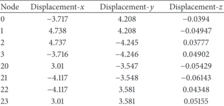
The second experiment was conducted on a beam with 90 nodes and 216 tetrahedral elements. Figures6(a)and6(b) show that the beam is constrained at the blue nodes and

(9)

(a) (b)

Figure 6: The beam mesh is constrained at the blue nodes and twisted at the green nodes. (a) Front view; (b) side view, which shows the force directions applied on each green node.

(a) (b)

(c) (d)

Figure 7: Nonlinear FEM results for the both the proposed and Pedersen’s methods ((a) wireframe tetrahedra and nodes; (b) nodes only; (c) wireframe surface mesh; and (d) shaded mesh).

Figure 8: The cross mesh is constrained at the blue nodes and pushed towards the green nodes.

twisted at both ends. Figure 7shows the final shape of the beam mesh for both the proposed and Pedersen’s methods. Tables3and4show the displacements at force applied nodes (green nodes) for the second experiment using the linear and nonlinear FEMs, respectively.

The third experiment was conducted with a cross mesh of 159 nodes and 244 tetrahedral elements. We aimed to observe if there is a root jump occurring when solving the system for a high amount of force (50 N units), and its effect

(10)

(a) (b)

Figure 9: Nonlinear FEM results for the both proposed and Pedersen’s methods: (a) initial and final wireframe meshes are overlaid; (b) initial and final shaded meshes are overlaid.

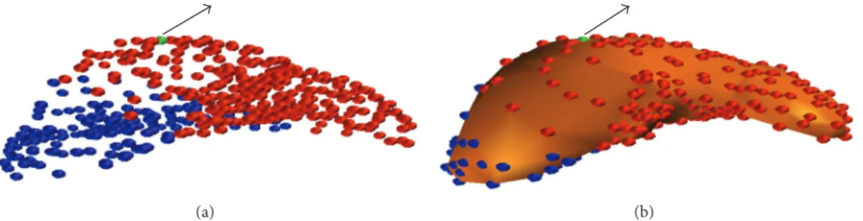
(a) (b)

Figure 10: The liver mesh is constrained at the blue nodes and pulled from the green node ((a) initial nodes; (b) initial shaded mesh and nodes).

Table 9: Computation times (in seconds) of stiffness matrices (Pedersen: Pedersen’s nonlinear FEM; Proposed: proposed nonlin-ear FEM; and Speed-up: relative performance comparison of the stiffness matrix calculation of the proposed nonlinear FEM method with Pedersen’s nonlinear FEM method using single thread).

Exp. Elements Pedersen Proposed Speed-up

1st 6 0.7322 0.3308 221.3422

2nd 216 28.1624 11.1542 252.4825

3rd 224 30.1094 12.2725 245.3404

4th 1580 239.8753 96.7840 247.8460

Table 10: Computation times (s) of system solutions (Pedersen: Pedersen’s nonlinear FEM; Proposed: proposed nonlinear FEM; and Speed-up: relative performance comparison of the proposed nonlinear FEM method with Pedersen’s nonlinear FEM method using single thread).

Exp. Elements Pedersen Proposed Speed-up

1st 6 3.0144 2.4427 123.4044

2nd 216 192.5288 159.6241 120.6139

3rd 224 586.2708 612.5911 95.7034

4th 1580 2840.7558 2401.0994 118.3106

Table 11: Newton-Raphson iteration count to reach desired accu-racy (Pedersen: Pedersen’s nonlinear FEM; Proposed: proposed nonlinear FEM).

Exp. Elements Pedersen Proposed

1st 6 5 5

2nd 216 7 7

3rd 224 26 32

4th 1580 8 8

on the computation times for both methods.Figure 8shows that the cross shape is constrained at the blue nodes and pushed towards the green nodes. Figure 9 shows the final shape of the beam mesh for both the proposed and Pedersen’s methods. Tables 5 and 6 show the displacements at force applied nodes (green nodes) using the linear and nonlinear FEMs, respectively.

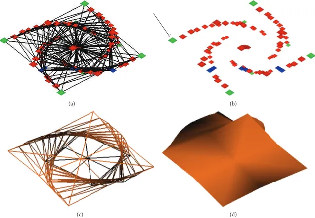
We conducted fourth experiment with a liver mesh of 465 nodes and 1560 tetrahedral elements. Figure 10 shows that the mesh is constrained at the blue nodes and pulled from the green node (30 N units) in the direction of the arrow. We aimed to observe the similar amount of speedup like previous experiments for a high density mesh. Figure 11 shows the final shape of the beam mesh for both the proposed and Pedersen’s methods. Tables7and8show the displacements at force applied node (node number 271) using the linear and nonlinear FEMs, respectively.

Computation times of the finite element experiments are required to compare how much faster our proposed method is than Pedersen’s. When comparing nonlinear FEMs, we calculated the computation times to construct the stiffness matrices as well as the computation times of the nonlinear FEM solutions to determine how different calculations affect them.Table 9depicts the computation times for the stiffness matrix calculation and Table 10 depicts the computation times for the system solution. Table 11 shows the iteration counts to solve the system using the Newton-Raphson pro-cedure.

The speed-up columns of Tables 9 and 10 depict the speedups of the proposed method compared to Pedersen’s method for the stiffness matrix calculation and the system solution using a single thread, respectively. The speedup is calculated as follows:

Speedup= Runtime(Pedersen’s method)

(11)

(a) (b)

Figure 11: Nonlinear FEM results for both the proposed and Pedersen’s methods: (a) left: wireframe surface mesh; right: wireframe surface mesh with nodes; (b) left: shaded mesh; right: shaded mesh with nodes.

(a) (b)

(c)

Figure 12: (a) Initial misshapen nose. (b) The head mesh is constrained at the blue nodes and pushed upwards at the green nodes. (c) The result of the nonlinear FEM: left: wireframe surface mesh with nodes; right: shaded mesh with texture.

Our proposed method outperforms Pedersen’s method. On the average, it is 142% faster at computing stiffness matrices because Pedersen’s method uses more symbolic terms. However, both methods use Newton-Raphson to solve nonlinear equations, which takes approximately90% of the computation time. Thus, the overall speedup decreases to 15% on average. In experiment 3, because of more iterations due to root jumps, there was a performance loss against Pedersen’s method.

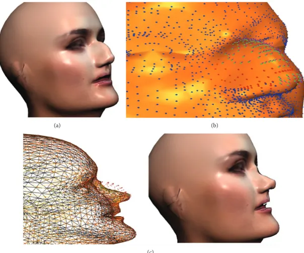
We also applied our method for corrective operation on the misshapen nose of a head mesh. The head mesh is composed of 6709 nodes and 25722 tetrahedral elements (see Figure 12(a)); all the operations were performed in the nose

area of only 1458 tetrahedral elements. Figure 12(b) shows that the head mesh is constrained at the blue nodes and pushed upwards at the green nodes andFigure 12(c)shows the result of the nonlinear FEM.

4. Conclusions and Future Work

We propose a new stiffness matrix calculation method for nonlinear FEM that is easier to analyze in terms of construct-ing elemental stiffness matrices and is faster than Pedersen’s method. The proposed method is approximately 2.4 times faster, on average, at computing stiffness matrices and15% faster at computing the whole system than Pedersen’s method.

(12)

Although the proposed nonlinear FEM has significant advantages over Pedersen’s nonlinear FEM, there is still room for the following development.

(1) Heuristics could be applied to avoid root jumps. (2) Although we decreased system memory usage by

simplifying the solution process for the nonlinear FEM, a significant amount of system memory is still used. The solution process could be further optimized to decrease memory usage.

Conflict of Interests

The authors declare that there is no conflict of interests regarding the publication of this paper.

References

[1] K.-J. Bathe, Finite Element Procedures, Prentice-Hall, Engle-wood Cliffs, NJ, USA, 1996.

[2] D. L. Logan, A First Course in the Finite Element Method, Cengage Learning, 5th edition, 2012.

[3] P. Pedersen, “Analytical stiffness matrices for tetrahedral ele-ments,” Computer Methods in Applied Mechanics and Engineer-ing, vol. 196, no. 1-3, pp. 261–278, 2006.

[4] G. R. Joldes, A. Wittek, and K. Miller, “Real-time nonlinear finite element computations on GPU: application to neurosur-gical simulation,” Computer Methods in Applied Mechanics and Engineering, vol. 199, no. 49–52, pp. 3305–3314, 2010.

[5] Z. A. Taylor, M. Cheng, and S. Ourselin, “High-speed nonlinear finite element analysis for surgical simulation using graphics processing units,” IEEE Transactions on Medical Imaging, vol. 27, no. 5, pp. 650–663, 2008.

[6] M. Cerrolaza and J. C. Osorio, “Relations among stiffness coefficients of hexahedral 8-noded finite elements: a simple and efficient way to reduce the integration time,” Finite Elements in Analysis and Design, vol. 55, pp. 1–6, 2012.

[7] J. Bonet and R. D. Wood, Nonlinear Continu um Mechanics for Finite Element Analysis, Cambridge University Press, Cam-bridge, UK, 1st edition, 1997.

[8] C. A. Felippa, “Lecture notes in nonlinear fin ite element meth-ods,” Tech. Rep. CUCSSC-96-16, Department of Aerospace Engineering Sciences and Center for Aerospace Structures, University of Colorado, 1996.

[9] P. Pedersen, The Basic Matrix Approach for Three Simple Finite Elements, 2008, http://www.topopt.dtu.dk/files/PauliBooks/ BasicMatrixApproachInFE.pdf.

[10] C. T. Kelley, Iterative Methods for Linear and Nonlinear Equa-tions, Frontiers in Applied Mathematics, Society for Industrial Mathematics, 1st edition, 1987.

[11] S. Krenk, Non-linear Modeling and Analysi s of Solids and Structures, Cambridge University Press, 1st edition, 2009. [12] The Mathworks, “Calling MATLAB Engine from C/C++

and Fortran Programs,” 2014, http://www.mathworks.com/ help/matlab/matlab external/ f38569.html.

[13] Autodesk, “3ds Max—3D Modeling, Ani mation, and Render-ing Software,” 2012, http://www.autodesk.com/products/auto-desk-3ds-max/.

[14] Maplesoft, “MATLAB Connectivity—Maple Features,” 2012,

http://www.maplesoft.com/products/maple/features/matlab-connectivity.aspx.

[15] E. Madenci and I. Guven, The Finite Element Method and Applications in Engineering Using ANSYS, Springer, Berlin, Germany, 1st edition, 2006.

(13)

Submit your manuscripts at

http://www.hindawi.com

Hindawi Publishing Corporation

http://www.hindawi.com Volume 2014

Mathematics

Journal of

http://www.hindawi.com Volume 2014 Mathematical Problems in Engineering

Hindawi Publishing Corporation http://www.hindawi.com

Differential Equations International Journal of

Volume 2014

http://www.hindawi.com Volume 2014 Hindawi Publishing Corporationhttp://www.hindawi.com Volume 2014

Mathematical PhysicsAdvances in

Complex Analysis

Journal of

Optimization

Journal of Hindawi Publishing Corporation

Combinatorics

http://www.hindawi.com Volume 2014 International Journal of Hindawi Publishing Corporation

Journal of

Function Spaces

Abstract and Applied Analysis Hindawi Publishing Corporation

http://www.hindawi.com Volume 2014 International Journal of Mathematics and Mathematical Sciences

Hindawi Publishing Corporation http://www.hindawi.com Volume 2014

The Scientific

World Journal

Discrete Dynamics in Nature and Society

Discrete Mathematics

Journal of

http://www.hindawi.com Volume 2014 Hindawi Publishing Corporationhttp://www.hindawi.com Volume 2014

Fast Stiffness Matrix Calculation for Nonlinear Finite Element Method

Research Article